Numerical study of forebody wake effect on axisymmetric parachute opening shock and drag reduction

ABSTRACT

Parachute–forebody distance is a parameter which is amongst the most critical factors to be considered in forebody wake effect. In this study, a new axisymmetric parachute–forebody coupling model is developed. Axisymmetric wrinkling membrane element is built to assess the dynamic response of the parachute canopy membrane under fluid pressure. Besides, fluid model and its further implementation on the fluid structure analysis are discussed. With the proposed method, the wake effect on both the opening shock during inflation state and the drag reduction during steady state can be obtained efficiently. Finally, numerical model is validated with published experimental result and further employed to investigate the influence of distance parameters on fluid–parachute coupling behaviour. On the basis of numerical results, failure distance during the inflation process and critical forebody–parachute distance are determined. The results show that forebody–parachute distance has a strong influence on flow behaviour around the parachute in both inflation state and steady descent state.

KEYWORDS:

• Parachute inflation
• axis symmetric
• forebody wake effect
• drag reduction

Nomenclature

Dp:	=	Constructed canopy diameter
Lfp:	=	Distance between the forebody and the leading edge of the parachute
u:	=	Point displacement vector
X:	=	Point position vector
Cd:	=	Drag coefficient of the parachute with forebody
Cd,∞:	=	Drag coefficient of the parachute without forebody
Cf:	=	Drag coefficient of the forebody
v∞:	=	Free stream velocity
Closs:	=	Ratio of drag coefficient with forebody to drag coefficient without forebody
Rf:	=	Forebody radius
Lf:	=	Trailing length of the forebody
Lp:	=	Trailing distance ahead of the parachute
m:	=	Gores number of the parachute
h:	=	Thickness of the parachute membrane
k:	=	Turbulent kinetic energy
ε:	=	Turbulent dissipation
$\tilde{v}$:	=	Fluid mesh moving velocity
$\bar{v}$:	=	Average velocity of the fluid
${\mathbf{v}}^{\prime }$:	=	Fluctuations velocity of the fluid
$\upsilon$:	=	Fluid kinematic viscosity

1. Introduction

Since parachutes are much simpler and more effective than other aero decelerators, deceleration systems based on parachutes systems are widely used as an effective air drop for deploying personnel as well as cargo during a combat operation or even otherwise. The main purpose of a parachute is to decelerate a payload to a lower speed aerodynamically. In the deceleration application, the payload, also known as the forebody, will affect the flow field and bring about a new vortex distribution over the canopy.

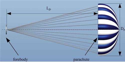
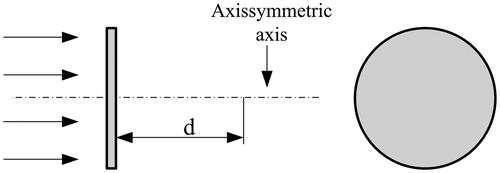
The change of flow field resulting from forebody is termed forebody wake effect. According to Knacke’s study [1], the reduction in parachute drag due to the forebody influence ranges from 2% to 70%. This range of parachute drag reduction is primarily dependent on the forebody size and the distance between the forebody and the leading edge of the parachute, which is termed forebody–parachute distance for the sake of simplicity. The design for the suspension line length is dependent on the forebody–parachute distance, as depicted in Figure 1. Therefore, the forebody wake effect should be fully considered before the parachute designing and its optimization.

Figure 1. Parachute–forebody structure.

In an airdrop performance, a decelerator system usually experiences three divided states：the deployment state, the inflation state and the steadily decent state. The forebody wake has a significant influence on the inflation state as well as on the steady descent state. Herein the study on the forebody wake effect should focus on two phases during the parachute performance. And these two phases include the inflation phase and the steady descent phase which will be discussed in details as follows.

Parachute inflation phase is a very special one when parachute fabric materials can undergo large and arbitrary deformation in a very short time. The inflation characteristics investigation is carried out through experiments in the early study [2–4]. With the continuous development of numerical algorithms and the computer hardware, it brings tremendous savings in time and cost of parachute simulating and thereby FSI problem of the parachute has been attracting scholars’ attention. Irvin Aerospace initiated a strategy to develop an analysis methodology that enabled parachutes to be simulated in a virtual fluid environment. And models developed in finite element code LS-DYNA were performed in both infinite and finite mass scenario [5–7]. In addition, similar investigation can be found at Kim’s works. At his works, parachute inflation was simulated with immersed boundary method [8–10]. Yu [11] and Cheng [12] studied the inflation of a parachute with SALE (simple ALE) method and experimentally validated the results. Fan numerically studied the parachute based on non-linear finite element method and preconditioning finite volume method. The results obtained with these methods agreed with the experiments well.

However, there exists one shortcoming for these methods, namely, Eulerian mesh must span the entire range of the activity associated with the Lagrangian structure while the number of these Eulerian elements must be sufficient to permit the fluid to flow into the closed mouth of the canopy in packed condition. This would surmount a very large number of elements and hence a high computing cost. For instance, the parachutes test ranging from 3.5 ft to 9 ft takes around 0.9 million elements to fulfil the task [7]. For this reason, although the foregoing mentioned successful studies have been made to analyse the inflation state of parachute, the wake effect during this state is usually omitted for the sake of computational expediency. Therefore, the wake effect on the inflating parachute is rarely studied and reported. In this article, however, in order to study the wake effect, a axisymmetric model is developed, which is suggested by the inherent axisymmetric geometry of the parachute. This study assumes a circumferentially averaged axisymmetric flow leading to the solution of a two-dimensional problem in the meridional plane. The axisymmetric model can be considered as the ‘’bridge‘’ between one- and three-dimensional design procedures for the parachute, and provides an optimal compromise between computational cost and fidelity of the results [13–15]. Based on this simplification, the forebody wake effects during the inflation process are studied by virtue of this efficient developed model.

After parachute inflation process terminates, the fluid keeps on interacting with the parachute until an equivalent state is achieved, which is termed steady descent state. During this state, the presence of the wake vortex dramatically makes the dynamic pressure inside canopy decrease. Many researchers have proposed various approaches to describe the wake effect in steady descent state. Heinrich et al. [16] originally described the reduction in parachute drag through giving an empirical velocity distribution. Peterson and Johnson further improved the method through experiments study [17]. In addition to these empirical results, Anita Sengupta provided a cost-efficient aerodynamic performance database that captured the wake effect of the Orion crew module on the parachute through subscale model experiment [18]. McQuilling et al. [19] presented time-resolved and time-averaged results from simulations using a Reynolds-averaged Navier-Stokes (RANS) flow solver to study the effects of a forebody wake on the aerodynamics of the double annular parachute. Based on a simple ‘immersed boundary technique’, Xiao et al. investigated the effects of suspension lines on the supersonic flow field [20]. These methods provide a tool to study the forebody wake effect in steady descent phase. However, the effect of suspension line and forebody are not considered in the inflation state.

In this article, the forebody wake effect is studied numerically through establishing the axisymmetric forebody–parachute coupling model. Both inflation case and steady decent case can be reflected in the present analysis. With this method, not only can the flow behaviour of the forebody wake be clearly observed, but also new criteria that help to judge the fluid topology around the forebody and parachute are provided.

This article is organized as follows. In the first section, the axis symmetric finite element model is developed to facilitate opening a parachute. In the second section, an axisymmetric finite membrane structure element is established and discussed. In the third section, the fluid model as well as the coupling method will be outlined. And the inflated method will be presented. Moreover, the challenge such as the efficiency problem can be solved in this axisymmetric configuration. Finally, the forebody wake effect in both inflation state and steady descent state is discussed.

2. Mathematical equation of the axisymmetric membrane

In this section, an axisymmetric finite membrane structure element is established and discussed. With this element, the canopy is modelled by a series of elements whose geometries are axisymmetric. These elements are subjected to axially symmetric loading conditions. A dynamic model of the canopy is established based on the following assumptions:

1. Thickness of the membrane is invariant.

2. The membrane cannot stand any bending.

3. The forebody is fixed.

4. The suspension line effect is neglected.

5. The parachute shape is invariable after it is fully inflated.

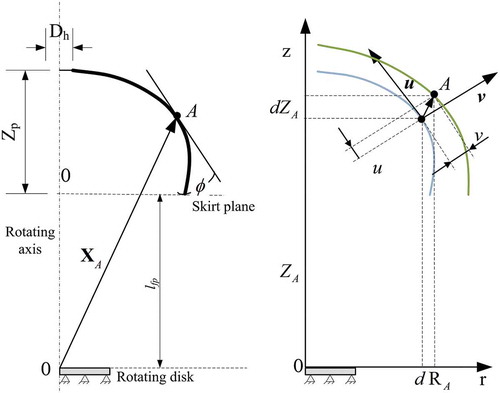
The forebody shape is determined by engineering practice [17,18,21,22]. In this model, the forebody is modelled as a rotating disk for the sake of simplicity, as depicted in Figure 2.

Figure 2. Position and displacement of the parachute.

After the parachute is fully inflated, the steady descent state is achieved. Breathing phenomenon as well as the fly out angles variant will totally bring about 5%–20% reduction in parachute drag. However, according to Knacke’s study, the reduction in parachute drag due to the forebody influence ranged from 2% to 70%. Since this article is more concerned about the trailing distance, the parachute shape is assumed as invariable after it is fully inflated for the sake of simplicity and stability. And the effect of the breathing phenomenon is cancelled numerically.

According to the foregoing assumptions, the axisymmetric parachute can be modelled by rings of constant cross-sections. The centre of all nodal circles is on the z-axis, which is the axis of revolution. The directions of mechanical displacements are represented by r, θ, z, which are the radial, circumferential and axial coordinates, respectively. The origin is located at the centre of the disk. The structure deformation is outlined in terms of this inertial frame. As shown in Figure 2, let e_r, e_z be unit vectors in radial, and axial directions. A is an arbitrary point of the canopy. u and X denote displacement and position vector of this arbitrary point, respectively.

The position of the arbitrary point A can be represented as

(1) $\mathbf{X}=R{\mathbf{e}}_r+\mathrm{Z}{\mathbf{e}}_z$(1)

And the displacement of the point can be represented as

(2) $\mathbf{u}=u{\mathbf{e}}_r+w{\mathbf{e}}_z$(2)

The general theory of thin membrane is used to represent the dynamics of very flexible thin membrane structures. Let V denote a volume occupied by a part of the body in the current configuration. The displacement formulation for stress analysis is based on the energy concept of finding u that both satisfies the essential boundary conditions on u and minimizes the total energy. The virtual strain and kinetic energies are written as

(3) $\underset{V}{\int }\left(\delta U+\delta T+\delta W\right)dV=0$(3)

In the expression above, T and U are kinetic and internal energy densities per unit volume, respectively, and W is the virtual work of applied loads per unit volume. The weak form can be written as

(4) $\underset{\nu }{\int }\left[\delta {\epsilon }^{\mathrm{T}}\sigma +\delta {\mathbf{u}}^{\mathrm{T}}\left(\mathbf{f}-\rho \ddot{\mathbf{u}}\right)\right]dV+\underset{s_{\sigma }}{\int }\delta {\mathbf{u}}^{\mathrm{T}}\bar{\mathbf{f}}dS=0$(4)

The equilibrium formulation requires the expression of strain and stress. The relations of strain and displacements are given by the linear part of Green–Lagrange strain tensor in cylindrical coordinates, which take the following form

(5) $\epsilon ={\left(\begin{array}{cc}{\epsilon }_s& {\epsilon }_{\theta }\end{array}\right)}^{\mathrm{T}}=\mathbf{B}\mathbf{u}$(5)

(6) $\sigma =\mathbf{D}\epsilon$(6)

A piece of membrane can support large tensile forces but is weak at supporting torque. As the membrane cannot stand any bending, shear stress is neglected, which greatly simplifies the model. Thus the shear strain no longer exists in this inflation model on purpose. With the foregoing assumptions, the membrane equation matrix B can be written as

(7) $\mathbf{B}=\left[\begin{array}{cc}cos\varphi \frac{\mathrm{\partial }}{\mathrm{\partial }s}& sin\varphi \frac{\mathrm{\partial }}{\mathrm{\partial }s}\\ 0& 1/r\end{array}\right]$(7)

(8) $\begin{array}{ccc}cos\varphi =dZ/ds& and& sin\varphi =dR/ds\end{array}$(8)

where s is the meridian length along the canopy.

Researchers do come up with a relatively simple and meanwhile a productive parachute structural model by taking advantage of some specific construction features of a circular parachute. When the membrane is wrinkling, tension is lost in one principal direction and canopy fabric cannot support any stresses. Thus it’s assumed that the canopy membrane piece cannot bear circular tensile stress until it is fully inflated. Taut stresses only engage when the current distance between the axis of symmetry and the radius position of point is greater than the final shape function of the parachute.

(9) $\begin{array}{cc}\mathbf{D}=\frac{Eh}{1-{\nu }^2}\left[\begin{array}{cc}1& c\nu \\ \nu & c\end{array}\right]& c=\left\{\begin{array}{c}\begin{array}{cc}0& R(s)\le \eta (s)\end{array}\\ \begin{array}{cc}p& R(s)>\eta (s)\end{array}\end{array}\right. \end{array}$(9)

E is the Young’s modulus of the membrane, ν is Poisson’s ratio and p is the penalty factor of the parachute expansion. The parachute ceases stretching with large penalty factor after inflation. η is the radius between the node and the symmetry axis of an inflated parachute, which describes the fully inflated shape of the parachute. h is the thickness of the membrane. The fully inflated shape is determined by the structure of the parachute. Without using the CALA (CANOPY LOADS ANALYSIS) logic proposed by Sundberg [23], the final shape in this article is calculated with FEM code by imposing a constant pressure. After the FEM code has found the values of nodes displacement, the approximation value of the η(s) at node i is obtained, which is denoted as $\tilde{\eta }(S_i)$. The field variable η(s) can be approximated with NURBS interpolation [24].

The membrane mass is obtained through the undeformed Gore profile, as depicted in Figure 3. Therefore, the virtual work of inertia force is written as followed

(10) $\underset{V}{\int }\delta {\mathbf{u}}^{\mathrm{T}}\rho \ddot{\mathbf{u}}dV=\underset{s}{\int }\delta {\mathbf{u}}^{\mathrm{T}}2m\rho hL(s)\ddot{\mathbf{u}}ds$(10)

Figure 3. Undeformed Gore profile of a round parachute.

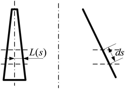
where L is the distance between the seam and the symmetric axis of the Gore; m is the number of gores; The virtual work of the aerodynamic force is obtained as followed

(11) $\underset{V}{\int }\delta {\mathbf{u}}^{\mathrm{T}}\mathbf{f}dV=\underset{s}{\int }\delta {\mathbf{u}}^{\mathrm{T}}2\pi R(s)\mathbf{P}(s)ds$(11)

where P is the pressure difference across the membrane.

(12) $\mathbf{P}={\left[\begin{array}{cc}Psin\varphi & Pcos\varphi \end{array}\right]}^{\mathrm{T}}$(12)

To solve the above equations the canopy domain is discretized into a number of elements. The Lagrange interpolation is used to construct the shape function of the element. The position and displacement is written as

(13) $\mathbf{u}={\mathbf{N}}_j{\mathbf{u}}_j$(13)

where N_j is the shape function matrix of node j.

Equation (8) can be written as

(14) $\begin{array}{ccc}cos\varphi =\frac{1}{J}\frac{dZ}{d\xi }& and& sin\varphi =\frac{1}{J}\frac{dR}{d\xi }\end{array}$(14)

(15) $J=ds/d\xi =\sqrt{{\left(dR/d\xi \right)}^2+{\left(dZ/d\xi \right)}^2}$(15)

where $\xi \in [-1,1]$ is normalized coordinate of an element.

Based on this analysis, an updated parachute position can be obtained when the pressure is given. For the purpose of comparing with the aerodynamic loads distribution of the elastic parachute, the parachute is divided into many segments along the meridian shape.

3. Mathematical equations of the fluid coupling model

3.1 Formulation of fluid model

The structure model requires a pressure distribution along the meridional length of the canopy as input. It is more efficient to obtain a reliable solution with numerical computational fluid method. The flow field is governed by the continuity and momentum equations. The incompressible NavierStokes (NS) equations are written as

(16) $\mathrm{\nabla }\mathbf{v}=0$(16)

(17) $\frac{\mathrm{\partial }\mathbf{v}}{\mathrm{\partial }t}+\mathrm{\nabla }\mathbf{v}\mathbf{v}=-\frac{1}{\rho }\mathrm{\nabla }p+\upsilon {\mathrm{\nabla }}^2\mathbf{v}$(17)

where ρ is the fluid density, v, p, υ are velocity, static pressure and kinematic viscosity of fluid respectively. Ormieres [25] discussed the relationship between Reynolds number and turbulent wake of a sphere. The critical Reynolds number is about 800. Namely, when an external flows around spherical obstacles, its Reynolds number is beyond this critical number, and the turbulent wake will appear after the sphere. As depicted, the inflated shape of a typical circular parachute can be assumed as an hemispherical shell, and its Reynolds number is over 1000. Therefore, the flow characteristic is considered as turbulent, and turbulence model is added [26].

Decomposing the N-S equations into the RANS equations makes it possible to simulate engineering fluid dynamic problems. In this article, the Standard k-epsilon model is implemented to simulate this engineering fluid dynamic problem. This model is RANS equations-based turbulence models.

Decompose the pressure and the velocity into mean and fluctuations

(18) $\mathbf{v}=\bar{\mathbf{v}}+{\mathbf{v}}^{\prime }$(18)

where $\bar{\mathbf{v}}$ is the average velocity and ${\mathbf{v}}^{\prime }$ is the fluctuations velocity

The fluctuations are lumped into the kinetic energy

(19) $k=∥{\mathbf{v}}^{\prime }∥/2$(19)

The turbulent kinematic eddy viscosity is introduced, which is given as

(20) ${\upsilon }_T=C_1{k}^2/\epsilon$(20)

where k is the turbulent kinetic energy, and ε is the dissipation.

The average velocity and the average pressure are solved by

(21) $\frac{\mathrm{\partial }}{\mathrm{\partial }t}\bar{\mathbf{v}}+\mathrm{\nabla }\cdot \bar{\mathbf{v}}\bar{\mathbf{v}}=-\frac{1}{\rho }\mathrm{\nabla }p+(\upsilon +{\upsilon }_{\mathrm{T}}){\mathrm{\nabla }}^2\bar{\mathbf{v}}$(21)

In order to enclose the equations, turbulent kinetic energy and dissipation are solved by

(22) $\mathrm{\partial }k/\mathrm{\partial }t=\mathrm{\nabla }\cdot (\upsilon +C_2{\upsilon }_{\mathrm{T}})\mathrm{\nabla }k-{\tau }_{ij}\mathrm{\partial }\bar{v}/\mathrm{\partial }{x}_j-\epsilon$(22)

(23) $\mathrm{\partial }\epsilon /\mathrm{\partial }t=\mathrm{\nabla }\cdot (\upsilon +C_3{\upsilon }_{\mathrm{T}})\mathrm{\nabla }\epsilon +C_4\left(\epsilon /k\right){\tau }_{ij}(\mathrm{\partial }{\bar{v}}_i/\mathrm{\partial }{x}_j)-C_5{\epsilon }^2/k$(23)

(24) ${\tau }_{ij}=\frac{2}{3}k{\delta }_{ij}-{\upsilon }_{\mathrm{T}}\left(\frac{\mathrm{\partial }{\bar{v}}_i}{\mathrm{\partial }{x}_j}+\frac{\mathrm{\partial }{\bar{v}}_j}{\mathrm{\partial }{x}_i}\right)$(24)

where constants are given as C₁ = 0.09, C₂ = 1, C₃ = 1.3, C₄ = 1.44, C₅ = 1.92 [27]. The formulation is applied to the forebody fluid simulation.

ALE formulation of the parachute is necessary due to the large deformation taking placed in the parachute inflation state. The moving grid methods are performed [28–30], as depicted in Figure 4.

(25) $\frac{\mathrm{\partial }}{\mathrm{\partial }t}\bar{\mathbf{v}}+\mathrm{\nabla }\cdot \bar{\mathbf{v}}\left(\bar{\mathbf{v}}-\tilde{\mathbf{v}}\right)=-\frac{1}{\rho }\mathrm{\nabla }\bar{p}+(\upsilon +{\upsilon }_{\mathrm{T}}){\mathrm{\nabla }}^2\bar{\mathbf{v}}$(25)

Figure 4. ALE formulation and mesh moving.

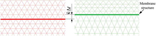
where $\tilde{v}$ is the fluid nodes moving velocity. This velocity stems from the structure boundary motion. The axisymmetric incompressible turbulent N-S equations is modified as below

(26) $\frac{1}{r}\frac{\mathrm{\partial }}{\mathrm{\partial }r}(r{\bar{v}}_r)+\frac{\mathrm{\partial }{\bar{v}}_z}{\mathrm{\partial }z}=0$(26)

(27) $\left(\frac{\mathrm{\partial }{\bar{v}}_r}{\mathrm{\partial }t}+u_r\frac{\mathrm{\partial }({\bar{v}}_r-{\tilde{v}}_r)}{\mathrm{\partial }r}+u_z\frac{\mathrm{\partial }({\bar{v}}_r-{\tilde{v}}_r)}{\mathrm{\partial }z}\right)=-\frac{\mathrm{\partial }p}{\mathrm{\partial }r}+(\upsilon +{\upsilon }_{\mathrm{T}})\left[\frac{1}{r}\frac{\mathrm{\partial }}{\mathrm{\partial }r}(r\frac{\mathrm{\partial }{\bar{v}}_r}{\mathrm{\partial }r})+\frac{{\mathrm{\partial }}^2{\bar{v}}_r}{\mathrm{\partial }z}-\frac{{\bar{v}}_r}{r^2}\right]$(27)

(28) $\left(\frac{\mathrm{\partial }{\bar{v}}_z}{\mathrm{\partial }t}+u_r\frac{\mathrm{\partial }({\bar{v}}_z-{\tilde{v}}_z)}{\mathrm{\partial }r}+u_z\frac{\mathrm{\partial }({\bar{v}}_z-{\tilde{v}}_z)}{\mathrm{\partial }z}\right)=-\frac{\mathrm{\partial }p}{\mathrm{\partial }z}+(\upsilon +{\upsilon }_{\mathrm{T}})\left[\frac{1}{r}\frac{\mathrm{\partial }}{\mathrm{\partial }r}\left(r\frac{\mathrm{\partial }{\bar{v}}_z}{\mathrm{\partial }r}\right)+\frac{{\mathrm{\partial }}^2{\bar{v}}_r}{\mathrm{\partial }{z}^2}\right]$(28)

In this article, the far-field free stream condition is applied and the normal velocity boundary condition is set. The solution method is implicit formulation finite volume method. This method is used to spatial discrete the space of fluid field. Second-order upwind scheme is used on convection and turbulent viscosity terms. Through computation, the aerodynamic parameters of every parachute segment are obtained.

3.2 Coupling solution procedure

After the fluid model is established, it will be coupled with the structural model discussed in Section 2. In this article, a two-way coupling method is applied [31]. The coupling approach in the parachute model is explicit in time. During each time step in the coupled run the CFD and structural dynamic computations are advanced one time step. First of all, fluid meshes are updated based on the updated canopy surface representation. The meshes are defined by repositioning the surface boundary as well as the outer boundary of the parachute, and then updating interior nodes and nodes along the axisymmetric axis. Next, pressure distribution on two sides of the parachute is updated. Second, with the new pressure difference, the motion of the membrane can be obtained. The process is repeated over and over again, until a termination condition is achieved. With this procedure, additional insight into parachute–fluid behaviour is achieved using the proposed finite element model.

4. Example and discussion

4.1 Inflation state analysis

4.1.1 Validation of numerical inflation process

With application of the numerical model developed, simulations of the flow around the parachute are now carried out. The structure code and the coupling system are implemented with ANSI C [32]. And we resort to the commercial CFD solver Fluent to complete the fluid dynamic computation.

In order to validate the inflation process, comparison is made with respect to experimental data provided by Desabrais’s experiments [33]. The experiments were performed in a water tunnel which has internal dimensions of 0.6 m wide by 0.6 m deep by 2.4 m long. Diameter of parachute is 30.5 cm. The weight of cloth is 37.3 g/m², and the thickness of fabric is 500 μm. The material of the fabric and suspension line is rip-stop nylon and nylon, respectively. The opening force is compared with the experiment results provided by Desabrais’s experiments [33], as depicted in Figure 5.

Figure 5. Time history of the vent hole parachute force.

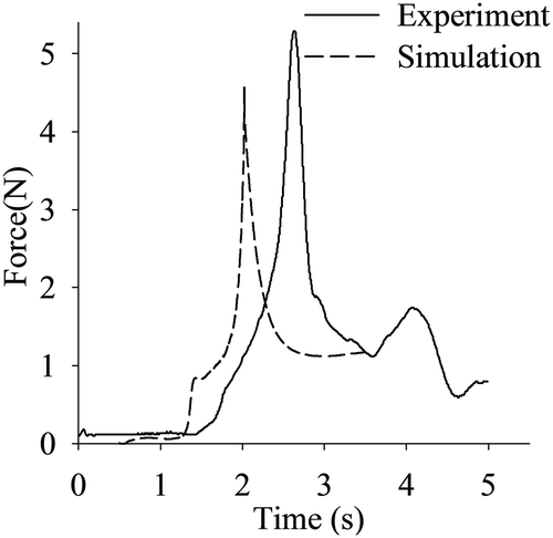
The opening shock obtained with the simulation process accords with the tendency of the experiments. Parachute FSI simulation results show agreement with experimental results and previous literature, and thus qualify the method developed in this article to be applicable with large-scale parachute. This validated model is applied to the following full-scale parachute analysis.

4.1.2 Forebody wake effect during the inflation process

When the parachute inflation process terminates, steady decent state begins and the parachute is found to be fully inflated. From the initial state to fully inflated state, the parachute experiences large deformation. During this inflation process, volume expansion of the parachute leads to the pressure plummeting. The pressure difference between inside and outside of the parachute forces the fluid around the parachute to get into the canopy. When the forebody is placed ahead of the parachute, the fluid accumulates ahead of the forebody instead of flowing into the canopy. Some of the fluid bypasses obstacles and fills the low-pressure region inside the canopy. However, this part of fluid is quite limited when the forebody stays close to the parachute. In this example, a D_f = 1.6 m diameters round disk is chosen and an D_p = 5.6D_f diameter parachute is selected. The surrounding fluid is air and the free stream velocity is 20 m/s. The material of the computational domain is air. The computational domain is 12 m along radius direction and 96 m along the axial direction. The fluid domain is discredited with about 5e4 cells.

When the forebody disk stays close to the parachute, the fluid is difficult to flow into the canopy and the canopy may fail to inflate, as depicted in Figure 6. When no forebody is placed ahead of the parachute, the parachute is inflated successfully. However, when the distance between the disk plane and the parachute skirt is 2.8D_f, the parachute shrinks and fails to expand.

Figure 6. Parachute inflation process.

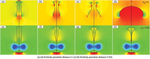
Figure 6 shows the failure process of a parachute with a placed 2.8D_f from the skirt. Owing to this obstacle, most of the fluid cannot successfully fills the quasi-vacuum region and the low pressure inside the canopy forces the parachute to shrink at the opening mouth. However, when the parachute begins its shrink at the opening mouth, it becomes even more difficult to fill the canopy. All in all, to guarantee the safety of the decelerator system is the primary task of airdrop system design, and the distance between the parachute and the forebody cannot be too close.

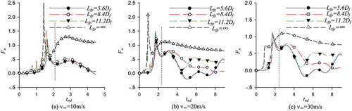
Non-dimensional forebody–parachute distance varies from 5.6D_f to 11.2D_f to explore the effect of wake coupling on the parachute flow. The free stream velocity varies from 10 m/s to 30 m/s.

Figure 7 shows time histories of parachute opening forces under free stream velocity condition are 10 m/s, 20 m/s, and 30 m/s, respectively. In order to provide a thorough comparison of the wake reduction, the nominal shock is applied. The nominal shock is present in non-dimensional form

(29) $F_n=2F(t)/(\rho v^2\pi D_p^2)$(29)

Figure 7. Opening shock with different free stream velocity.

The non-dimensionalize time is given as followed

(30) $t_{nd}=t{V}_{\mathrm{\infty }}/D_p$(30)

According to the assumption (5) in the second section, canopy structures do not change after it has fully expanded. Namely, the influence of breathing phenomenon has been eliminated and the forebody placement is the main reason that results in the difference between opening forces. Through the results, the parachute achieves a stable flow field and drags force quickly without forebody, while with the forebody, the parachute opening force will experience plummeting. The topology [34] of the vortexes can also be observed in Figure 8. The flow field drastically changes with time when the forebody is placed near the parachute skirt.

Figure 8. Variant of the flow topology according to time.

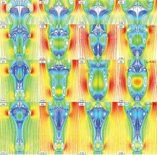
The main source of instabilities originates in the turbulence interaction between the vortexes of the forebody and the canopy [35]. Through Figure 8 (a)–(d), when there is no disk placed ahead of the parachute the drag converges quickly and varies slowly after it is fully inflated. However, the drag caused by the canopy behaves differently when a forebody is placed ahead of the parachute. It is shown that the opening force varies enormously when the forebody is closer to the parachute and the flow field becomes less stable. Vortices begin shedding and it takes a long time for the vortices to separate and combine with other vortices until it achieves the balance state.

4.2 Steady-state analysis of forebody–parachute structure

After the parachute is fully inflated, the parachute achieves a new balance state descent steadily. In this state, parachute drag reduction is primarily dependent on the ratio of forebody diameter to parachute diameter as well as the distance between the forebody and the leading edge of the parachute. With the turbulent model mentioned above, the predominate flow features could be identified and obtained numerically. In order to study relationship between these parameters and the drag loss effect, the flow behaviour around the forebody as well as the parachute in steady descent phase will be presented and discussed in this example.

4.2.1 Steady-state analysis of forebody

Since the ratio of forebody diameter to parachute diameter is an important parameter that affects the flow topology, this study will focus on the wake effect determination of forebody size.

A single rotating disk suffering constant velocity stream is investigated numerically. The basic radius of this disk is 1.0 m, as depicted in Figure 9.

Figure 9. Structure of the forebody.

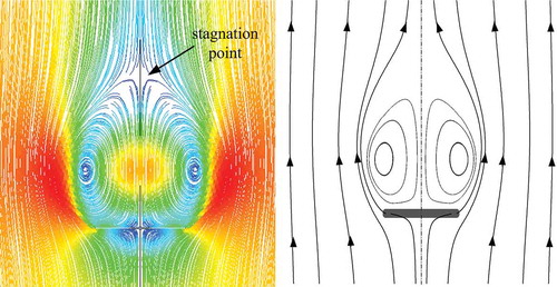
The forebody is considered as a bluff body. As depicted in Figure 10, the flow topology of a single forebody is present. It can be observed that there is a vortex ring placed behind these bluff bodies. There is a stagnation point located at the topic of vortexes rings. At stagnation point, the velocity as well as the pressure is zero. The fluid begins to separate at this point which is located at the axisymmetric axis. Therefore, the relationship between the forebody size and its stagnation point position is investigated through pressure and velocity distribution along the axisymmetric axis. These relations are present to manifest the flow characteristic and its corresponding structure.

Figure 10. Flow topology of a single forebody.

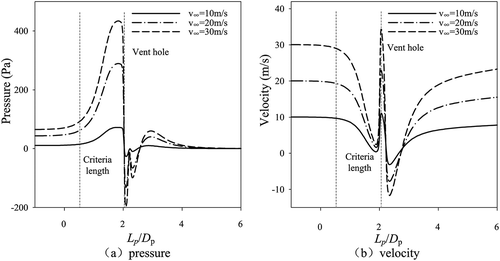
In Figure 11, pressure and velocity distribution with different forebody radius along the axisymmetric axis are present. Non-dimensional distance which varies from 0 to 5D_f is present to discuss the forebody wake effect. Computations are conducted for D_f from 1 m to 4 m. The free stream velocity is 20 m/s.

Figure 11. Pressure and velocity distribution with different forebody radius.

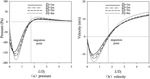
Through Figure 11, it is shown that the pressure increases slowly after the initial decrease. The velocity is almost zero at stagnation point. Therefore, it can be observed that stagnation point is located at approximately L_f = 1.75D_f to forebody. The forebody effect decays according to distance and can almost be neglected at 5D_f. In this example, it can be observed that there is a linear relation between the forebody size and the stagnation point distance.

The relationship between stagnation point distance and the free stream velocity is also present. Figure 12 shows pressure and velocity distribution along the axis symmetric axis with different free stream velocity ranging from 10 m/s to 30 m/s. It is obvious that the location of the stagnation point is independent from the free stream velocity. In this example the stagnation points are also located at approximately 1.75D_f to the round disk.

Figure 12. Pressure and velocity distribution with different velocity.

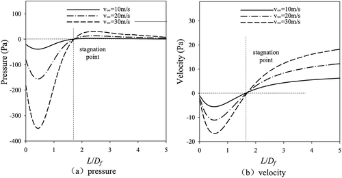
According to these results, it can be concluded that the free stream velocity has little effect on the stagnation point location. The trailing distance decays with distance and has a linear relation to forebody size.

4.2.2 Steady state of parachute

The flow topology of one single parachute is present in Figure 13 [36,37]. The pressure and velocity along parachute axis under free stream velocity 10 m/s, 20 m/s, 30 m/s are shown in Figure 14. The fluid jets at vent hole and an obvious vortex ring are formed behind the canopy. Similar to the single forebody analysis, the investigations of flow characteristic are carried out through studying its pressure and velocity distribution along the axisymmetric axis. As a bluff body, the pressure increases, the fluid velocity decelerates inside the canopy, and the fluid is accumulated.

Figure 13. Fluid topology of a single parachute.

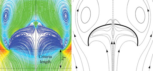
Figure 14. Velocity and pressure distribution along the parachute.

The effect that the parachute acts on the fluid can be neglected at the point located at approximately L_p = 1.0D_p distance ahead of the canopy skirt.

4.2.3 Steady state of parachute–forebody structure

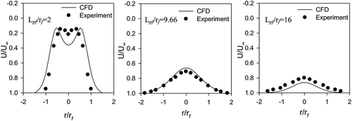
First of all, the velocity along the radius axis is compared with the velocity profiles obtained through the experiment with wind tunnel [17]. Figure 15 shows that the computed velocity distribution accords well with the experimental distribution during the steady state. CFD model can be applied to further study the system parameters, such as the forebody diameter and the distance between forebody and parachute leading edge.

Figure 15. Experimental and CFD velocity distributions behind forebody.

When the fluid is blocked by the forebody, the flow behaviour around the parachute with block is quite different from that around the forebody free parachute. Researchers have employed different approaches to describe the forebody effect. For instance, Heinrich studied the measured values of parachute drag loss and gave simplified turbulent wake velocity distribution equations [17]. Peterson studied the experiment results and gave the modified expressions for forebody configurations.

(31) $C_{loss}=\frac{C_d}{C_{d,\mathrm{\infty }}}=1+\frac{2}{R_f^2}\frac{D_1}{D_2}\left(1-e^{D_2{R}_f^2}+\frac{D_1}{4}{e}^{2D_2{R}_f^2}-\frac{D_1}{4}\right)$(31)

where the parameter is given as $D_1=a/(L_{fp}/2R_f{)}^m$, $D_2=-1/\left(0.435b^2\right)(L_{fp}/2R_f{)}^{2n}$; a and b are exponential functions of forebody drag coefficient.

(32) $\begin{array}{cc}a=0.42{\mathrm{e}}^{0.99{\mathrm{C}}_f}& b=0.54{\mathrm{e}}^{0.84{\mathrm{C}}_f}\end{array}$(32)

Fix the forebody–parachute distance L_fp = 11.2D_f, and the ratio of forebody diameter to parachute diameter which varies from 0.05 to 0.25D_p is studied numerically. The drag loss results are compared with the empirical function results, as shown in Figure 16.

Figure 16. Drag loss vs. forebody radius.

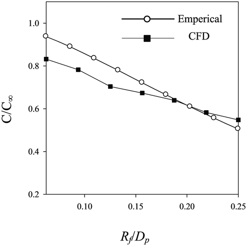
The results achieved by CFD method have a fine agreement with those obtained through the empirical function. It can be concluded that both empirical function and CFD method can be applied to predict the drag loss feature when the forebody is far away from the parachute.

However, when the forebody is getting close to the parachute, the drag loss manifests great distinctions between two methods, as shown in Figure 17, the result is obtained as free stream velocity is 20 m/s and the forebody radius is 0.7 m. It is assumed that parachutes are fully inflated and no vortexes shedding takes place. Runs are made as forebody–parachute distances range from 5.6 to 11.2D_f.

Figure 17. Drag loss vs. forebody–parachute distance.

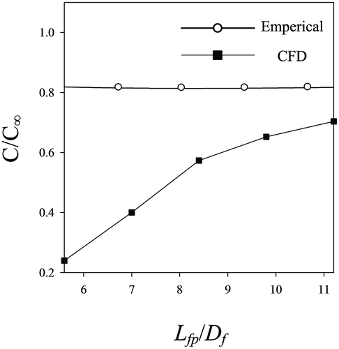
The tendency of CFD result is more align to comparative experiment data obtained by Knacke. When the forebody is approaching the parachute, large drag loss occurs. However, the results obtained through empirical data cannot provide a similar tendency, as shown in Figure 17. The poor agreement between present CFD data and empirical predictions points out that the empirical analysis may be insufficient to cover all the drag loss cases when the forebody is approaching the parachute. In this study, a generalized correlation for the variation of drag loss with L_fp has been developed for the cases in which the forebody approaches the parachute and the flow changes. Subsequently, the critical value of L_p at which the onset of vortex separation takes place is identified with both the length of stagnation point vortex L_f and parachute distance L_p. The criteria distance L_fp can be approximated by the summation of these two values.

${\tilde{L}}_{fp}=L_f+L_p$

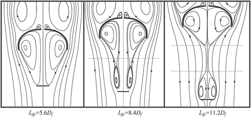
When the parachute–forebody distance is much larger than this criteria distance, the vortexes ahead of the parachute and vortex behind the forebody will separate. The pressure loss effect is minor. However, when the forebody gets close to the parachute and the distance is smaller than the criteria value, these vortexes will combine and lead to the parachute drag loss. The fluid stream is present in Figure 18. The vortex begins to separate with distance ${\tilde{L}}_{fp}$. The topology evolution according to the distance is present in Figure 19.

Figure 18. Stream path with different forebody–parachute distance.

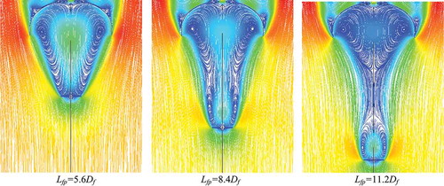
Figure 19. Flow topology with different forebody–parachute distance.

In this example, the drag loss will be alleviated with the larger distance. However, when the distance is greater than 11.2D_f, the forebody wake effect is quite limited. And the drag force may be difficult to benefit from the increase of the distance L_fp.

5. Conclusions

A forebody–parachute model is developed and applied to the numerical analysis. The parachute in both inflation and steady descent state is discussed. In addition, the fluid response of forebody–parachute structure for various distances is considered. Through computation results, there are several conclusions drawn as follows.

1. With the simplified axisymmetric forebody–parachute model, the forebody wake effect in both inflation and steady state can be obtained efficiently.

2. When the parachute is inflating, if the parachute is close to the forebody, the parachute may fail to inflate, or experience an unstable state for a long time.

3. There is a separating point located on the forebody–parachute system. When vortex shedding does not take place, the parachute will experience considerable drag loss due to vortex combination. And when the forebody–parachute distance is larger than the criteria distance, the drag loss effect will decay or alleviate.

Disclosure statement

No potential conflict of interest was reported by the author.

Additional information

Funding

This study is supported by the National Natural Science Foundation of China [No. 11472137].

References

- T.W. Knacke, Parachute Recovery Systems: Design Manual, Para Pub, Santa Barbara, CA, 1992.
- P.S. Jason and A. Hart, Canned telemetry system for sensor data on parachute system, AIAA. 15 (2005), pp. l3.
- Y. Li, Z. Xinhua, and L. Shuisheng, Experimental on canopy payload performance of parachute, J. Beijing Univ Aeronaut. Astronaut. 33 (10) (2007), pp. 1178.
- L. Yu, X. Ming, and B. Hu, Experimental investigation in parachute opening process, J. Nanjing Univ. Aeronaut. Astronaut 38 (2) (2006), pp. 176–180.
- B.A. Tutt and A.P. Taylor. The use of LS-DYNA to simulate the inflation of a parachute canopy.18th AIAA Aerodynamic Decelerator Systems Technology Conference and Seminar. 2005.
- Y. Fan and J. Xia, Simulation of 3D parachute fluid–structure interaction based on nonlinear finite element method and preconditioning finite volume method, Chin. J. Aeronautics 27 (6) (2014), pp. 1373–1383. doi:10.1016/j.cja.2014.10.003
- B. Tutt, S. Roland, R.D. Charles, and G. Noetscher, Finite mass simulation techniques in LS-DYNA, 21st AIAA Aerodynamic Decelerator Systems Technology Conference and Seminar, Dublin, 2011, pp. 2592.
- J. Kim, Y. Li, and X. Li, Simulation of parachute FSI using the front tracking method, J. Fluids Struct. 37 (2013), pp. 100–119. doi:10.1016/j.jfluidstructs.2012.08.011
- Y. Kim and C.S. Peskin, 3-D parachute simulation by the immersed boundary method, Comput. Fluids 38 (6) (2009), pp. 1080–1090. doi:10.1016/j.compfluid.2008.11.002
- Y. Kim and C.S. Peskin, 2-D parachute simulation by the immersed boundary method, SIAM J. Scientific Comput. 28 (6) (2006), pp. 2294–2312. doi:10.1137/S1064827501389060
- L. Yu, H. Cheng, Y. Zhan, and S. Li, Study of parachute inflation process using fluid–structure interaction method, Chin. J. Aeronautics 27 (2) (2014), pp. 272–279. doi:10.1016/j.cja.2014.02.021
- H. Cheng, X.-H. Zhang, L. Yu, and M. Chen, Study of velocity effects on parachute inflation performance based on fluid–structure interaction method, Appl. Math. Mech. 35 (9) (2014), pp. 1177–1188. doi:10.1007/s10483-014-1852-6
- K.R. Stein and R.J. Benney, Parachute inflation: A problem in aeroelasticity, DTIC Document, 1994.
- K.R. Stein, R.J. Benney, and E.C. Steeves, A computational model that couples aerodynamic and structural dynamic behavior of parachutes during the opening process, DTIC Document, 1993.
- L. Yu and X. Ming, Study on transient aerodynamic characteristics of parachute opening process, Acta Mech Sin 23 (6) (2007), pp. 627–633. doi:10.1007/s10409-007-0112-3
- H.G. Heinrich and T. Riabokin, “Analytical and experimental considerations of the velocity distribution in the wake of a body of revolution”. 1959, DTIC Document.
- C.W. Peterson and D.W. Johnson, Reductions in parachute drag due to forebody wake effects, J. Aircr. 20 (1) (1983), pp. 42–49. doi:10.2514/3.44826
- A. Sengupta, B. Goree, E.B. White, J. Guthery, R. Machin, G. Bourland, J. Laguna, R. Sinclair, and E. Hennings, Performance of a Subscale CPAS Conical Ribbon Drogue Parachute in a Turbulent Wake, AIAA Aerodynamic Decelerator Systems (ADS) Conference, Reston, VA, 2013, pp. 1307.
- M. McQuilling and J. Potvin. Forebody wake effects on the aerodynamics of an annular parachute. 42nd AIAA Fluid Dynamics Conference and Exhibit. 2012.
- X. Xue, H. Koyama, Y. Nakamura, and C.-Y. Wen, Effects of suspension line on flow field around a supersonic parachute, Aerosp. Sci. Technol. 43 (2015), pp. 63–70. doi:10.1016/j.ast.2015.02.014
- E.S. Ray and A.L. Morris. Measurement of CPAS main parachute rate of descent. 21st AIAA Aerodynamic Decelerator Systems Technology Conference. 2011.
- G. Guglieri, Parachute–payload system flight dynamics and trajectory simulation, Int. J. Aerosp. Eng. 2012 (2012), pp. 1–17. doi:10.1155/2012/182907
- W.D. Sundberg, New solution method for steady-state canopy structural loads, J. Aircr. 25 (11) (1988), pp. 1045–1051. doi:10.2514/3.45701
- L.A. Piegl and W. Tiller, The NURBS Book, Springer, Berlin, 1997.
- D. Ormières and M. Provansal, Transition to turbulence in the wake of a sphere, Phys. Rev. Lett. 83 (1) (1999), pp. 80–83. doi:10.1103/PhysRevLett.83.80
- A. Prosperetti and G. Tryggvason, Computational Methods for Multiphase Flow, Cambridge University Press, New York, 2007.
- H.K. Versteeg and W. Malalasekera, An Introduction to Computational Fluid Dynamics: The Finite Volume Method, Pearson Education, Edinburgh Gate, Harlow, 2007.
- E. Lefrançois, A simple mesh deformation technique for fluid–structure interaction based on a submesh approach, Int. J. Numer. Methods. Eng. 75 (9) (2008), pp. 1085–1101. doi:10.1002/nme.v75:9
- F.J. Blom, Considerations on the spring analogy, Int. J. Numer. Methods Fluids 32 (6) (2000), pp. 647–668. doi:10.1002/(ISSN)1097-0363
- K. Stein, T. Tezduyar, and R. Benney, Mesh moving techniques for fluid–structure interactions with large displacements, J. Appl. Mech. 70 (1) (2003), pp. 58–63. doi:10.1115/1.1530635
- L.K. Abbas, D. Chen, and X. Rui, Numerical calculation of effect of elastic deformation on aerodynamic characteristics of a rocket, Int. J. Aerosp. Eng. 2014 (2014), pp. 1–11. doi:10.1155/2014/478534
- N.M. Josuttis, The C++ Standard Library: A Tutorial and Reference, Addison-Wesley, Upper Saddle River, NJ, 2012.
- K.J. Desabrais, Velocity field measurements in the near wake of a parachute canopy. ProQuest dissertations and theses; Thesis–Worcester Polytechnic Institute, 2002.
- X. Pan, L. Hu, and Y. Cao, Analysis of dynamic simulation and fluid field of parachute in inflation stage, J. Aerosp. Power. 1 (2008), pp. 015.
- R. Ross and F. Nebiker, Survey of aerodynamic deceleration systems, 3rd Annual Meeting, Boston, MA, 1966, pp. 988.
- C. Jiang, Influence of low angle of attack on the flowfield characteristics of an axisymmetric parachute in terminal descent. Chin. Space Sci. Technol. 27 (2007), pp. 59–65.
- J.C.C.Y. Wenhan, The flowfield characteristics of an axisymmetric parachute in terminal descent, Spacecr. Recovery Remote Sens. 3 (2005), pp. 004.