Object-oriented modelling of wind turbines and its application for control design based on nonlinear dynamic inversion

ABSTRACT

This article presents the object-oriented modelling of wind turbine aero-elastics. The article details the undertaken modelling approach and demonstrates its validity by comparing the results to a domain-specific simulation tool. The resulting object-oriented models can be generically adapted to meet different tasks or combined with models from other domains. Also the combination object-oriented Modelica and functional mock-up interface technology enable a rapid design of nonlinear controllers. As one possible application example, the article presents the model-based design of a corresponding controller. Its goal is to extend the turbine lifetime by reducing the structural loads. To this end, a modern control scheme is proposed that takes full advantage of the underlying object-oriented modelling approach. The controller is based on nonlinear dynamic inversion control methods combined with pseudo control hedging. The controller uses wind speed measurement information to adjust to wind gust load. Simulation-based comparisons to conventional control designs show a large potential reduction of the gust load on the wind turbine using the proposed controller.

KEYWORDS:

• Elastic wind turbine modelling
• nonlinear dynamic inversion
• pseudo control hedging
• optimization
• blade-element momentum theory
• rotor aerodynamics

1. Introduction

Wind energy has become an important energy source with worldwide growing capacities. Research on advanced control design or net integration aims to help to improve the energy generation or extend turbine lifetime. Mathematical models of wind turbine support this development on various levels. Whereas relatively simple models form the basis for controller design, more complex models are needed for tasks of virtual validation and verification. Modern object-oriented equation-based languages such as Modelica [1] enable the development of model libraries that can cover this full application domain.

The required modelling effort for a complex machine like a wind turbine can be reduced considerably by the use of the object-oriented Modelica language. Users can build models of different complexity directly from provided library components and parameterize them as required. In addition Modelica also supports the generation of inverse system models which can be used as part of advanced control systems. This article describes the newly developed DLR¹ Modelica library dedicated to wind turbines and also shows how an inversion-based nonlinear controller can be designed using components of the library.

Section 2 describes the approach used for modelling the elastic wind turbine at various level of complexity using the Modelica language [1]. Section 3 then describes how the established blade element momentum theory (BEMT) can be formulated in an object-oriented manner and combined with other components. The inversion-based controller is described in Section 4 using Modelica and the functional mock-up interface (FMI) technology [3]. Simulation results and a comparison to a conventional scheduled controller are given in Section 5. A conclusion and outlook is given in section 6.

2. Modelling of elastic wind turbines

Modern wind turbines represent multi-domain systems. Hence, to describe the dynamic behaviour of a complete turbine, expertise from different areas is required: wind field analysis is needed to describe the environment; rotor-aerodynamics models the transformation of wind energy into kinetic energy; this kinetic energy is then turned into electric energy by the means of gears, electric machines and power system converters; also the flexibility of the tower structure and the blades needs to be taken into account.

Figure 2 illustrates how all these components are ultimately assembled for a complete turbine model within Modelica. It represents one specific example of a wind turbine that is based on the 5MW reference turbine from NREL [4]. The electric parts of the turbine (generator, converter and grid) have been adapted to the specifics of the European market.

Figure 1. Visualization of a Modelica Wind Turbine model using the DLR SimVis Library [2].

Figure 2. Top level Modelica model diagram of a typical wind turbine architecture.

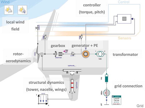
Given any task, the modeller will need to adapt this turbine model to her or his specific needs. For instance, modelling the integration of a turbine into electric grid requires more detailed modelling of the generators and converters, whereas for the task of this article, the generator can simply be represented as a controlled source of limited torque. It is thus necessary that each part of the turbine can be modelled with the appropriate level of complexity and detail. To ensure this flexibility, the modelling work is supported by a DLR library dedicated to wind turbines. In this library, DLR offers its combined modelling know-how in the field of drive-train [5], aerodynamics [6], structural dynamics [7], and visualization [2] (see Figure 1) in order to offer a complete system dynamics library for wind turbines. The following sections describe those parts of the library which are relevant for the control task at hand. These are: the modelling of the aerodynamics, the structural dynamics and the design of a standard controller.

2.1. Wind turbine aerodynamics

The evident key-component of a wind turbine is its rotor. The most-straight forward approach is to regard this component as one single entity that transforms wind energy into kinetic energy by a coefficient of efficiency $C_P$. This coefficient is typically defined as a function of the tip-speed ratio $\lambda$, expressing the relation between wind speed and the tip speed of the blades. If we take the collective pitch of the blades into account, we get a two-dimensional function, where both input parameters are subject to control laws: the pitch angle is controlled by the pitch actuators and the tip speed can be regulated by the power-off take of the generator. Hence, this basic model of a rotor is well applicable for classic control tasks.

For more advanced tasks, the rotor is decomposed into its blades and the blades are decomposed into blade elements. Each such element then has its own airfoil polar that describes the aerodynamic forces for lift and drag dependent on the angle of attack within the induced wind field. The induced wind field is a superposition of the global wind in the vicinity of the rotor field and the wind that is induced by the rotor itself. For a certain induced wind, the momentum needed to change the wind velocity and the momentums emanated from the aerodynamic forces of the blade element are equal. This equilibrium can be described by a nonlinear system of equations and forms the basis of the well-established BEMT method [8]. It is suitable for wind turbines without strong cross-winds or significant local turbulences. It can be used to take the influence of wind shear into account and to design individual pitch control systems. In combination with flexible blades and towers, good estimation of the structural loads can be performed.

For the method’s implementation in Modelica, a model of a local blade element has been created. In interaction with a global outer model for the rotor plane, this component determines the local aerodynamic forces. The individual blade elements can then be connected (rigidly or by a flexible body) to form a complete blade. Typically, three such blades then form the rotor. Details of this approach are described in Section 3.

2.2. Structural dynamics of tower and blade

Modern, large-scale wind turbines have rotors of more than 100 m of diameter. The flexibility of such a large structure is an integral part of its design. Most important are the structural dynamics of those components which are most exposed to the wind: the tower and the blades. The flexibility of the nacelle, especially of the mounting of its devices and bearings, is currently not considered but the elasticity of the nacelle mounting on its tower is taken into account around the yaw angle.

For the modelling of these components, the DLR FlexibleBodies Library [7] is used. Using this library, the components can be modelled using standard connectors of the Modelica Standard library. The blade-elements of the rotor aerodynamics can hence be connected to a flexible blade as well as to a rigid blade.

The components of the FlexibleBodies library are based on a modal approach. Structural information of the blade and tower stiffness, as presented in [4] can be incorporated into the model by a standard input data (SID) file [9]. Nonlinear effects such as the increased stiffness due to centrifugal stretching can be taken into account. The performance characteristics are comparable to the approach presented in [10].

2.3. Complete turbine model

For the control task of this article, the aerodynamics and structural elasticity are the key components of the wind turbine. Nevertheless, more components are needed to form a complete model. This is also shown in Figure 2. Wind models are needed that prescribe the regional wind conditions but also model local effects like height dependent wind shear and the tower dam effect. Components for gearbox, emergency brake, generator and power electronics form the complete drive train of the turbine model. Many different designs for such drive trains exist in current wind turbines and the presented diagram just shows one possible setup.

Finally, the controller of the turbine model is depicted in Figure 2 with its signals controlling motor torque and pitch angle. One possible and advanced design of such a controller is presented from Section 4 onwards but before a closer look on the implementation of the rotor-aerodynamics is of interest.

3. Object-oriented implementation of the blade-element momentum theory

In Section 2.1 the principle of the blade element momentum theory has been quickly outlined. This theory has been implemented for many applications in wind energy and is described in different sources [8,11,12] that also include a variety of extensions or modifications for different operation points. Typically, these implementations have been realized in specialized software such as FAST [11]. What, however, is still of interest, is how to implement this theory in a truly object-oriented framework and how to formulate the model equations in a form that is applicable for all foreseeable operation conditions (including corner cases such as zero-wind speed, counter-rotation, etc.). It reveals that alterations to commonly used forms are, therefore, required. One resulting benefit of the object-oriented Modelica approach is that wind turbines can then be simulated using generic Modelica simulation tools and that consequently the simulation can easily be combined with the simulation of power networks, other power plants and consumers without the need for further specialized tools.

3.1. Desired component in an object-oriented framework

The ideal blade element represents a massless entity that based on its own speed and the local wind-speed exhibits the corresponding aerodynamic forces and torques on a connector. The connector is thereby a set of variables for the position, orientation, forces and torques of an arbitrary component in three-dimensional (3D) space.

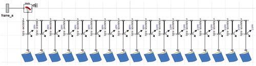
Once implemented, this blade element (cf. Figure 3) can then be combined with existing standardized components for multi-body simulation and flexible body simulation in order to model its mass and the motion of the complete rotor mounted on a tower. One possible model for a flexible blade is shown in Figure 4. Rigid blades can be modelled correspondingly.

Figure 3. Model icon of an individual blade element.

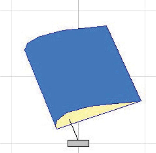
Figure 4. Model of a blade composed out of 17 blade elements and a flexible beam representing mass and structure.

3.2. Basic geometry of a blade element

The following subsections detail the model equations for the blade element starting with its geometrical features.

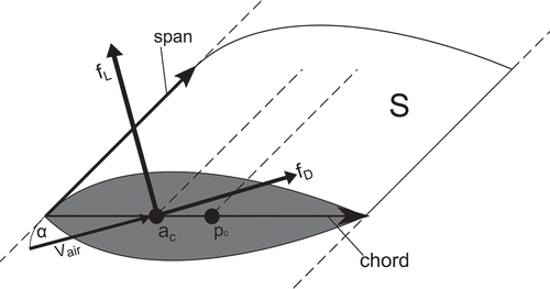
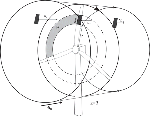
As illustrated in Figure 5, a blade element represents a section of the blade. It is represented by a 2D surface in 3D space. This surface $S$ is defined by two vectors: the span vector goes along the leading edge and determines the width of the blade element. The chord vector points from the leading edge to the tail and thereby represents the depth of the blade element. Along the edge, there are two lines. One represents the pitch axes, the other the centre of the aerodynamic forces. Both are specified by a scalar representing its position on the chord.

Figure 5. Geometry of a blade element, with a${\hspace{0.17em}}_c$ denoting the centre of aerodynamic forces and the p${\hspace{0.17em}}_c$ the pitch axes.

3.3. Computing wind-speed and angle of attack

In order to compute the aerodynamic forces, the relative airspeed at the leading edge ${\mathbf{v}}_{\mathrm{a}\mathrm{i}\mathrm{r}}$ is needed and its angle of attack $\alpha$. The airspeed thereby contains three components: (1) the local wind-speed at the blade-element’s position ${\mathbf{v}}_{\mathrm{l}\mathrm{o}\mathrm{c}}$, (2) the speed of the blade element itself ${\mathbf{v}}_{\mathrm{b}\mathrm{l}\mathrm{a}\mathrm{d}\mathrm{e}}$, and (3) the induced wind speed by the rotor ${\mathbf{v}}_{\mathrm{i}\mathrm{n}\mathrm{d}}$. Any airspeed component flowing along the span is thereby ignored:

(1) ${\mathbf{v}}_{\mathrm{a}\mathrm{i}\mathrm{r}}={\mathbf{v}}_{\mathrm{l}\mathrm{o}\mathrm{c}}+{\mathbf{v}}_{\mathrm{i}\mathrm{n}\mathrm{d}}-{\mathbf{v}}_{\mathrm{b}\mathrm{l}\mathrm{a}\mathrm{d}\mathrm{e}}.$(1)

How to model and determine the induced wind-speed ${\mathbf{v}}_{\mathrm{i}\mathrm{n}\mathrm{d}}$ will be discussed in the next section. For the moment, let us assume that it is given.

Given the vector for the airspeed and the blade-element, we can then derive the angle of attack $\alpha$ using basic trigonometry. The aerodynamic forces then result out of a tabularized airfoil polar. The airfoil polar provides the coefficients for the aerodynamic forces: $C_L,C_D$. To achieve a reliable numeric solution, it is important that the airfoil polar is given for the complete 360${\hspace{0.17em}}^{\circ }$. This may require rough guess values for the coefficients outside the standard operating points that mostly represent static approximations of stall behaviour.

With the coefficients, the resulting aerodynamic forces can be computed as follows:

(2a) ${\mathbf{f}}_L=C_L|{\mathbf{v}}_{\mathrm{a}\mathrm{i}\mathrm{r}}{|}^{2}S\frac{\rho }{2}{\mathbf{e}}_L,$(2a)

(2b) ${\mathbf{f}}_D=C_D|{\mathbf{v}}_{\mathrm{a}\mathrm{i}\mathrm{r}}{|}^{2}S\frac{\rho }{2}{\mathbf{e}}_D,$(2b)

where $\rho$ is the air density, $S$ is the surface of the blade element, and ${\mathbf{e}}_L$ and ${\mathbf{e}}_D$ are the unit vectors pointing in direction of lift and drag.

3.4. Computing the induced wind by the rotor

The central element of the blade-element momentum theory is that at the rotor plane, there is an induced wind generated by the rotor itself. If we focus on the wind component that is normal to the rotor plane (in direction of ${\mathbf{e}}_n$ as illustrated in Figure 6), this effect will change the upstream wind velocity from $v_{n,1}$ before the rotor plane to the downstream velocity $v_{n,3}$ behind the rotor plane. On the plane itself we assume the wind to be $v_{n,2}=(v_{n,1}+v_{n,3})/2$. Further we assume that the upstream velocity is the local wind velocity $v_{n,1}={\mathbf{e}}_n{\mathbf{v}}_{\mathrm{l}\mathrm{o}\mathrm{c}}$. It follows that ${\mathbf{v}}_{\mathrm{i}\mathrm{n}\mathrm{d}}=1/2(v_{n,3}-v_{n,1}){\mathbf{e}}_n$

Figure 6. Wind velocities in the rotor induced wind field.

In many implementations $v_{n,3}$ is not explicitly computed but instead $v_{n,2}$ is expressed by applying an induction factor $a$ on $v_{n,1}$: $v_{n,2}=a{v}_{n,1}$. This formulation is however problematic for small or zero wind velocity $v_{n,1}$. Hence, in this implementation $v_{n,3}$ is computed in order to derive ${\mathbf{v}}_{\mathrm{i}\mathrm{n}\mathrm{d}}$.

The $\mathrm{\Delta }v=v_{n,1}-v_{n,3}$ is causing a change of momentum of the air mass flow $\left|\dot{m}\right|$ caused by the aerodynamics of the blade element. The rate of the change has then to equal the aerodynamic forces in thrust direction ${\mathbf{e}}_n$:

(3) $({\mathbf{f}}_L+{\mathbf{f}}_D)\cdot {\mathbf{e}}_n=\left|\dot{m}\right|\mathrm{\Delta }v,$(3)

where $\left|\dot{m}\right|$ can be determined by the amount of air passing through the area $P$ of the rotor plane that is covered by the (assumed) full rotation of the blade element. $P=2\pi rspan/z$ with $z$ being the number of blades. Using $\left|\dot{m}\right|$ instead of $\dot{m}$ results from the underlying assumptions that the stream is going from upstream to downstream. Meaning, if the flow direction would change, so would the positions of $v_{n,1}$ and $v_{n,3}$. In order to determine $\left|\dot{m}\right|$, we can use the wind at the rotor plane $v_{n,2}$:

(4) $\left|\dot{m}\left|=\rho P\right|v_{n,2}\left|=\frac{\rho }{2}P\right|v_{n,1}+v_{n,3}\right|.$(4)

This will result in the following equation for the aerodynamic thrust:

(5) $({\mathbf{f}}_L+{\mathbf{f}}_D)\cdot {\mathbf{e}}_n=\frac{\rho }{2}P\left|v_{n,1}+v_{n,3}\right|(v_{n,3}-v_{n,1}).$(5)

This equation is, however, problematic since it offers one to three different solutions $v_{n,3}$ for the same level of aerodynamic thrust (cf. Figure 4). Indeed only the right quadrant of this curve is valid for this particular example. The behaviour in the left quadrant is not only creating numerical problems of multiple solutions it also does not coincide with what you observe in measurements. This is because the mass-flow estimation of Equation (5) is only valid for a laminar, gradual flow reduction. Already from inductions factors of $a>0.4$, the airflow becomes turbulent. In such a flow regime, it is very difficult to make any valid statement for the mass flow $\left|\dot{m}\right|$ since further air from outside the rotor disc is involved and the blade-element momentum theory basically becomes inapplicable. Nevertheless, it is important to have a numerically sound formulation of Equation (4) that provides a unique mapping between the aerodynamic thrust and the induced wind because, for instance, local high induction factors as occurring at the wing tips shall not corrupt the complete rotor model.

To this end, let us use a thumb-rule for high induction factors $a$. This thumb rule is not fully valid but yields a regular equation system and a physically plausible behaviour.

We can take into account the additional mass flow by the turbulence by adding weighted absolute terms of the individual velocities:

(6) $\left|\dot{m}\left|=\frac{\rho }{4}P\right|v_{n,1}+v_{n,3}\left|+\right|v_{n,1}\left|+\right|v_{n,3}\right|,$(6)

and the following equation for the aerodynamic thrust:

(7) $({\mathbf{f}}_L+{\mathbf{f}}_D){\mathbf{e}}_n=\frac{\rho }{4}P\left(\left|v_{n,1}+v_{n,3}\left|+\right|v_{n,1}\left|+\right|v_{n,3}\right|\right)(v_{n,3}-v_{n,1}),$(7)

which can be approximated by the point symmetric curve (see Figure 7):

(8a) $({\mathbf{f}}_L+{\mathbf{f}}_D){\mathbf{e}}_n=\frac{\rho }{2}P(\left|v_{n,1}\right|v_{n,1}-\left|v_{n,3}\right|v_{n,3}),$(8a)

(8b) $\frac{2\left|v_{n,1}\right|v_{n,1}-({\mathbf{f}}_L+{\mathbf{f}}_D){\mathbf{e}}_n}{\rho P}=\left|v_{n,3}\right|v_{n,3}.$(8b)

Figure 7. Different momentum-based thrust-laws for $v_{n,1}=1$.

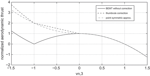
This formulation is now usable for all flow regimes. Although a plausible behaviour results, the validity of the models is however bad in turbulent situations but can be improved using additional correction factors originating from the Glauert [11] correction.

The aim of computing the induced wind ${\mathbf{v}}_{\mathrm{i}\mathrm{n}\mathrm{d}}$ is of course to take into account the effect on the angle of attack and the aerodynamic forces. This can be done by plugging in ${\mathbf{v}}_{\mathrm{i}\mathrm{n}\mathrm{d}}=1/2(v_{n,3}-v_{n,1}){\mathbf{e}}_n$, which makes also the aerodynamic forces on the left-hand side dependent on $v_{n,3}$. Since it involves $\alpha$ and the (tabularized) airfoil polar, the equation is difficult to solve and might have multiple solutions. Instead we propose to break this difficult nonlinearity by introducing a state for the induced wind velocity (see [13] for an elaboration of the general approach).

(9) $\frac{d{\mathbf{v}}_{\mathrm{i}\mathrm{n}\mathrm{d}}}{dt}T=-{\mathbf{v}}_{ind}+1/2(v_{n,3}-v_{n,1}){\mathbf{e}}_n,$(9)

with the time constant $T$ determining the speed for reaching the equilibrium. It is typically chosen to be order(s) of magnitude smaller than the minimum revolution time of the rotor. Then, it is possible to explicitly solve the unique solution for $v_{n,3}$:

(10) $v_{n,3}=ssqrt\left(\frac{\left|v_{n,1}\right|v_{n,1}-({\mathbf{f}}_L+{\mathbf{f}}_D){\mathbf{e}}_n}{\rho P}\right)$(10)

with $ssqrt(x):=sign(x)\sqrt{\left|x\right|}$.

The derivation has been performed here only for the component of the wind velocity that is normal to the rotor plane. The derivation can be also performed accordingly for the rotational component in the rotor plane. In this case the induced wind is represented by ${\mathbf{v}}_{\mathrm{i}\mathrm{n}\mathrm{d}}=1/2(v_{n,3}-v_{n,1}){\mathbf{e}}_n+1/2(v_{r,3}-v_{r,1}){\mathbf{e}}_r$. Furthermore, empiric correction factors can be applied similar to [11] in order to take into account for losses near the hub and blade tip.

3.5. Modelling common parameters and inputs for blade elements

While in principle each blade element computes the aerodynamic forces on its own, all blade elements share common parameters and inputs describing the corresponding rotor plane. These parameters can be collected in a global model and then be accessed within the blade-element.

This involves the following parameters:

• Number of blades $z$

• Time constant for the momentum equilibrium $T$

• $R$ for applying tip-loss correction factors

• $R_{hub}$ for applying hub-loss correction factorsand the following input

• ${\mathbf{e}}_n$ for the rotor plane

The global rotor model features a multi-body connector so that it can be connected to the hub: In this case also the yaw angle of the wind-turbine is taken into account.

Having such a blade-element component and this component for the global rotor parameters is what it takes for the object-oriented aeroelastic system modelling of a wind turbine. The remaining parts: the blades, the rotor, the nacelle, the tower, etc., can then be modelled using existing components from the Modelica Standard MultiBody Library [14] or the commercial flexible bodies library [7].

3.6. Model validation and performance

The resulting model of the wind turbine can be analysed with respect to its overall performance characteristics. The coefficient of performance $C_P$ expresses the fraction of the total wind power extracted by the turbine. Its theoretical optimum results from Betz’s law and is 0.59. The coefficient of thrust $C_T$ relates the thrust on the rotor to the thrust on a solid disc of the same radius. Both coefficients can be presented in a map with the two axes $\lambda$ and $\phi$. $\lambda$ is the speed of the rotor tip divided by the wind-speed, commonly denoted as tip-speed ratio. $\phi$ is the pitch angle of the blades.

To assess these maps, a grid of simulation runs has been performed. For the base model, the NREL reference turbine [4] with a constant, uniform wind-speed of 8 m/s was used. Prandtl losses for tip and hub as well as Glauert correction have been applied. The resulting maps are shown in Figures 8 and 9.

Figure 8. Coefficient of performance $C_P$. Solid lines are use for the Modelica model, dashed lines for FAST.

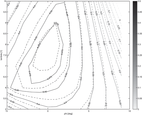
Figure 9. Coefficient of thrust $C_T$. Solid lines are use for the Modelica model, dashed lines for FAST.

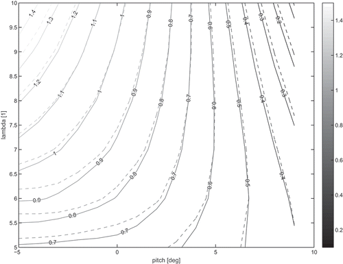
The plots display the performance maps for the presented Modelica model (being simulated using the simulation tool Dymola) and the FAST simulator [11] for wind turbines provided by NREL. Both maps show a good match between the different tools. The resulting differences are explained by a different implementation of the Glauert correction and by the application of different numerical ODE solvers. To further improve the validity of the presented models, real measurement data for different wind turbines designs would be needed. These are yet not available to us.

The range of $\lambda$ and $\phi$ in the presented maps corresponds to the extended typical operating range. Simulations for our models have also been performed way outside this range for $\lambda$ values from −10 to 20 and pitch angles from −25${\hspace{0.17em}}^{\circ }$ to 85${\hspace{0.17em}}^{\circ }$. For hundreds of such cases, the simulation succeeded successfully and returned good-natured and plausible results. This demonstrates the high numerical soundness of the presented models.

Having robust models also enables to perform a virtual test of the controller performance. As shown in the following sections, the controller design itself uses performance maps for the full rotor performance as internal model.

4. Using object-oriented modelling for the control of wind turbines

4.1. Introduction to the control task

While the nominal control of wind turbine is already well handled by the state of the art, and only minor improvements can be expected for the ideal case with smooth wind speed, there is still much potential in the field of load reduction. Especially under gust load conditions, the load on the flexible structure of the wind turbines can be reduced using advanced control methods.

One important aspect in this regard is the technological advance in wind speed measurement. Especially turbine-mounted light detection and ranging LIDAR-based wind speed sensors have become much more affordable and accurate. The measurement of the wind speed opens a wide range of control methods. Gust load can be substantial and induce strong vibrations of the wind turbine tower, which can lead to a lifetime reduction.

In recent years, many different advanced control approaches have been proposed for the control of wind turbines that use wind speed measurements [15]. Especially methods based on Model Predictive Control (MPC) strategies and feed-forward disturbance compensation methods show promising results, for example, [16–18].

In this work, we analyse nonlinear dynamic inversion (NDI) [19] combined with pseudo control hedging (PCH) [20] for the design of a controller and compare the approach to a standard controller setup in simulation. Similar controller structures are known from the field of aerospace control. Although not directly comparable, there are many similarities: in both cases the main source for the nonlinearity results from the changing wind speed (e.g. airspeed) and resulting aerodynamics. Actuator limits play a very important role (rates and absolute limits) and the excitation of the flexible structure has also to be considered in both cases during gust load situations.

Since good results have been achieved in the field of aerospace control using NDI with PCH, it is worthwhile to study its adaption and application for elastic wind turbines. One important aspect for the control of wind turbines are the dynamic ranges of the actuators. While the turbine generator can be controlled very fast to react to load changes, the pitch actuators of wind turbines are usually relatively slow. NDI has also recently been investigated for the pitch control of wind turbines [21] but we focus on the generator control, where a faster response can be achieved and use a two degree of freedom control system for the pitch control. The actuator to turn the wind turbine into the wind direction (yaw axis) is usually the slowest actuator and therefore not relevant for load mitigation control and will not be considered.

4.2. Control design

In this section the design of an advanced controller for the generator torque and blade pitch control will be described. The goal is to show how the performance of a benchmark 5-MW reference wind turbine (from [4]), especially under wind gust conditions, can be improved using modern control algorithms and wind speed measurements.

Table 1 shows the main properties of the wind turbine, which was modelled using the developed Modelica library, described in Section 2. The controller uses advanced features, such as the automatic inversion using the Modelica language and serves as an application example of the library. The benchmark setup as well as simulation results will be shown in Section 5.

Table 1. Properties for the NREL 5-MW baseline wind turbine taken from [4].

Rating	5 MW
Drive train	High speed, multiple-stage gearbox
Rotor, hub diameter	126 m, 3 m
Hub height	90 m
Cut-in, rated, cut-out wind speed	3 m/s, 11.4 m/s, 25 m/s
Cut-in, rated rotor speed	6.9 rpm, 12.1 rpm
Rated tip speed	80 m/s
Hub height	90 m
Rotor mass	110,000 kg
Nacelle mass	240,000 kg
Tower mass	347,460 kg
Rotor orientation, configuration	Upwind, three blades

The nonlinear characteristics of the wind turbine are considered in our model-based control design by using an inverse model of the wind turbine as part of the controller. The approach used here is NDI for the control of the generator torque together with PCH to handle actuator limits.

The basic idea of NDI is to eliminate the nonlinearity of a plant model by using an inverse plant model as part of the controller. The connection in series of the inverse plant model and plant acts as a linear system, such that a linear controller is able to handle the nonlinear plant without scheduling. Since the inverse model does not consider actuator limits, the basic concept of PCH is to have a parallel model of the plant which considers the actuator dynamic and limits. The difference between the desired signal and the resulting limited signal is then adjusted, using a reference filter and used to modify the desired input of the controller to stay within the limits.

The NDI notation and implementation used here is similar to [22–24] from the field of aerospace control, where also more details about NDI and PCH can be found.

An overview of the controller setup is shown in Figure 10, which will be explained in more detail in the following.

Figure 10. Overview of the combined NDI PCH control system for the generator torque in addition to a two degree of freedom pitch controller. The connections show the data flow between the different components.

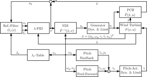
As an extension for the NDI and PCH control of the generator torque, a two degree of freedom control scheme is designed for the rotor pitch control, consisting of a feed-forward and feedback component.

For our controller design, it is assumed that measurement of the wind speed at the turbine is available. This could be based on LIDAR, for example, [25] or similar measurement methods in combination with additional estimators or filters. The exact estimation of wind speed and its use as part of a feed-forward controller is a difficult topic and still subject of ongoing research [17,26–28]. However big advances have been made in recent years and already quite promising results have been achieved in this field. Since the wind speed estimation is not our main research topic in this article, we will assume a reasonable estimation method is available and used. For our control design we assume a low-pass filtered wind speed measurement, to simulate that typical estimation methods will not be able to provide high frequency wind speed measurements.

The feedback controller design for the pitch control is based on the reference controller from [4] that will also be used for comparison of the controller performance in section 5. The reference pitch controller from [4] is a scheduled (on the generator speed) PI controller. Under nominal conditions the controller already works very well, but can be improved by a wind speed feed-forward controller addition.

The feed-forward controller for the pitch actuator consists of different elements: the main part is a linear interpolated table which contains a function ${\gamma }_{\mathrm{t}\mathrm{a}\mathrm{b}}(v_w)$ of optimal pitch actuator angles $\gamma$ depending on the measured wind speed. The optimal values are the steady-state results for a simulation using only the reference pitch controller and constant wind speed. Since the pitch actors are relatively slow, they should only be used when the generator is close to its limit. For this reason a switch is implemented in the feed-forward control law that only enables the controller close to the lower or upper limit of the generator speed (${\omega }_{g,\mathrm{l}\mathrm{o}\mathrm{w}}$ and ${\omega }_{g,\mathrm{h}\mathrm{i}\mathrm{g}\mathrm{h}}$). A hysteresis loop is implemented to avoid jittering of the switch close to the limit. When active, the output of ${\gamma }_{\mathrm{t}\mathrm{a}\mathrm{b}}(v_w)$ is used as input for a low-pass Bessel filter $G_{\mathrm{b}\mathrm{e}\mathrm{s}}(s)$ (Laplace variable $s$) and a rate limiter (limit ${\dot{\gamma }}_{c,\mathrm{m}\mathrm{a}\mathrm{x}}$) to ensure that the pitch actuators can follow the dynamics of the feed-forward controller:

(11a) ${\chi }_{\text{on}}={\omega }_g>{\omega }_{g,\text{high}}\vee \text{pre}({\chi }_{\text{on}})\wedge {\omega }_g>={\omega }_{g,\text{low}},$(11a)

(11b) ${\gamma }_{c,uf}=\{\begin{array}{cc}{\gamma }_{\text{tab}}(v_w),& \text{if}{\chi }_{\text{on}}=1,\\ 0,& \text{if}{\chi }_{\text{on}}=0,\end{array}$(11b)

(11c) ${\gamma }_{c,fi}=G_{\mathrm{b}\mathrm{e}\mathrm{s}}(s){\gamma }_{c,uf},$(11c)

(11d) ${\dot{\gamma }}_{c,ff}=\mathrm{m}\mathrm{i}\mathrm{n}\left(\mathrm{m}\mathrm{a}\mathrm{x}\left(\frac{{\gamma }_{c,fi}-{\gamma }_{c,ff}}{T_r},-{\dot{\gamma }}_{c,\mathrm{m}\mathrm{a}\mathrm{x}}\right),{\dot{\gamma }}_{c,\mathrm{m}\mathrm{a}\mathrm{x}}\right),$(11d)

(11e) ${\gamma }_{c,ff}=\int {\dot{\gamma }}_{c,ff}dt.$(11e)

Equation (11) shows the resulting equations and logic for the feed-forward controller. The feed-forward controller is combined with the scheduled PI pitch controller from [4] to form a two degree of freedom control system.

For the definition of the NDI and PCH generator control law we use the following notation: we assume the general nonlinear system description of the wind turbine in the form of Equation (1), where $x\in {\mathbb{R}}^n$ is the state vector, $u\in {\mathbb{R}}^k$ is the input vector, $y\in {\mathbb{R}}^l$ is the vector of outputs that are controlled, $p\in R^{n_p}$ are the parameters and known inputs of the system and $z\in {\mathbb{R}}^m$ contains any other outputs of the system. Any other control inputs are considered as known parameters ($\in p$). The nonlinear model is our implementation based on the 5-MW reference wind turbine from [4], using the model library described in Section 2.

(12a) $\dot{x}=f(x,p)+g(x,p)u,$(12a)

(12b) $y=h(x,p),$(12b)

(12c) $z=h_0(x,p).$(12c)

The inverse system can be generated using Lie-derivatives of the output $h$ along $f$ and $g$.

(13) $\dot{y}=L_{f}h(x,p)+L_{g}h(x,p)u.$(13)

Assuming that $L_g(x,p)$ is invertible and all outputs have the relative order 1 with respect to one of the inputs, the following control law can be constructed:

(14) $u_c={\left(L_{g}h(\hat{x},p)\right)}^{-1}\left({\dot{y}}_d-L_{f}h(\hat{x},p)\right).$(14)

In Equation (22) $y_d\in {\mathbb{R}}^l$ represents the demand rates and $\hat{x}$ represents a subset and estimation of the states $x$ of the original system.

(15) $\hat{x}=({\varphi }_g,{\omega }_g,\gamma ,\dot{\gamma },v_w{)}^T.$(15)

In the following, we will use a shortened notation where $F(x,u)$ is used for Equation (2), $\hat{F}(\hat{x},u)$ for a differentiable approximation of $F(x,u)$ for which all assumptions are valid. For $\hat{F}(\hat{x},u)$, the flexible dynamics are neglected and the tables used for the nonlinear aerodynamics are replaced by differentiable B-splines. For the modified system only a subset $\hat{x}$ of the states of the original system $x$ are used. The subset of the states $\hat{x}$ in Equation (23) consist of the generator angle ${\varphi }_g$ and angular velocity ${\omega }_g$, the pitch actuator angle $\gamma$ and angular velocity $\dot{\gamma }$ as well as the mean wind speed at the rotor blades $v_w$.

The inverse system based on $\hat{F}(\hat{x},u)$ and Equation (22) is called $F^{-1}\left(\hat{x},\nu \right)$ using the virtual control input $\nu =\dot{y}$. Using ${\hat{F}}^{-1}\left(\hat{x},\nu \right)$ to generate the input $u_c$ for $\hat{F}$ would lead in the ideal case (with $F=\hat{F}$ and all $p$ perfectly known) to an input/output linearization such that the original nonlinear system is transformed to a closed loop system with decoupled linear dynamics:

(16) $\dot{\widehat{x}}=\nu .$(16)

But even in the case if only $F\approx \hat{F}$ the nonlinearity of the closed loop system can be greatly reduced, such that a linear controller is better able to achieve good performance.

A main advantage of using the newly developed Modelica library for wind turbines for the design is that the inverse control law of Equation (14) can be generated automatically from a modified Modelica model of the wind turbine. Using the automatic differentiation and index reduction [29] features of Dymola [30] and the Modelica modelling language. The inverse model is then converted to an functional mock-up interface (FMI) [3] for which the states of the inverse system are transformed to additional inputs.

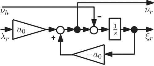
An outer control loop is used in combination with ${\hat{F}}^{-1}\left(\hat{x},\nu \right)$ to control the resulting dynamic of Equation (24) and to damp effects of modelling errors and parameter uncertainties. Since the actuators of wind turbines are limited and also have a dynamic behaviour additional measures are necessary. An approach similar to [22] and [23], from the field of aerospace, is used here. It consists of a reference filter $G_r(s)$ (Figure 11) and a model of the system $\hat{F}(\hat{x},u)$ in combination with a PID-feedback controller in the outer loop. The reference filter is used to modify the controller demand such that the actuator limits are maintained. To achieve this, a parallel model of the plant $\hat{F}(\hat{x},u)$ is used. The inputs for the parallel model are a subset of the measured states $\hat{x}$, defined in Equation (23), of the wind turbine $F$. The outputs of the reference filter are the set point ${\xi }_r$ for the $\lambda$-PID controller and a term ${\nu }_r$ that is directly added to the output $\nu$ of the PID controller. The reference filter is parameterized as a critical damped filter with cut off frequency $f_r$ (filter parameter $a_0=2\pi f_r$).

Figure 11. First order reference filter $G_r(s)$ for the PCH.

It is assumed that all these quantities are measurable or obtainable using an observer. For $\hat{F}$ the flexible dynamics of the wind turbine are neglected, that is, no elasticity of the powertrain and tower is considered in ${\hat{F}}^{-1}\left(\hat{x},\nu \right)$. This means ${\varphi }_g$ and ${\omega }_g$ can also be directly used to calculate the blade speed, except for a constant factor for the gear ratio $I_{\mathrm{g}\mathrm{e}\mathrm{n}}$ and tip speed ratio $\lambda ={\omega }_{g}R/v_w$ (rotor radius $R$).

There a multiple reasons for this approximation: If the elasticity of powertrain and especially the elasticity of the tower would be directly considered for ${\hat{F}}^{-1}$ the complexity would rise substantially. Although the inversion would still be possible, at least for a flexible powertrain using the automated inversion of Dymola, higher order derivatives of the inputs and equations of motion for the inverse model would be required (e.g. of $\lambda$, $v_w$, and $\gamma$). Since these are measurement values, it would make the inverse model very sensitive to noise and uncertainties in these quantities. For the NDI approach, additional measurements of the elastic deformations would then also be necessary (since the whole state vector is required for the method) that are often not readily available. In addition the computational time for the control algorithm would rise considerably, such that a real time implementation could be problematic. If elastic effects are considered, also the zero-dynamics of the system used for the inversion can be critical. A stable zero-dynamics is necessary for a stable inversion. The zero-dynamics can be approximated by the (transmission-) zeros of a linearization of the nonlinear system since the full nonlinear analysis of the zero-dynamics can usually not be solved analytically for complex systems (see [31] for details). For the rigid system, all zeros have no positive real part, and therefore do not turn into unstable poles for the inverse system. The reasons mentioned here are likewise main factors why NDI control systems in the aerospace field are usually also based on rigid models, even though the aircraft can show significant elastic deformations. The simplification of ${\hat{F}}^{-1}$ also reduces the number of parameters required for the tuning since the properties and parameters of a flexible wind turbine model are much more difficult to identify, compared to a rigid model.

For ${\hat{F}}^{-1}$ the inversion is done with respect to $\dot{\lambda }$, so that in Equation (14) $u_c={\tau }_g$ and $\dot{y}=\dot{\lambda }$. The tip speed ratio was chosen for the inversion since the optimal operation point can be found from $C_p$-$\lambda$ curves. The model used for the inversion is modified such that the highest derivatives that are required for the computation of the inverse model are directly used as inputs and connected to integrator chains of the respective order.

The parallel model used for the PCH algorithm is the same forward model $\hat{F}$ used to generate the inverse model ${\hat{F}}^{-1}$, but without the added integrator chains and re-defined inputs.

The resulting inverse model of the rigid wind turbine is then exported as an FMI. In the FMI-code, the state of the inverse system is redefined as an input such that no integration of the derivatives is necessary. The resulting inverse system is therefore in the form of Equation (22) . The required Lie-derivatives are solved automatically by Modelica/Dymola. The modified FMI can then be used for a controller implementation directly on target hardware, or can be re-imported into the Modelica/Dymola to simulate the complete control system. The implemented FMI can be computed much faster as real-time on a standard CPU and is therefore suited for controller implementation on a target hardware. To account for the actuator limits, the output of the inverse model $u_c$ is modified by limiter for the absolute value and the rate, using the same limiter equation as in Equation (11d) for the pitch rate $\dot{\gamma }$. The result is the generator torque $u$ that is used as set point for the wind turbine torque generator and the PCH parallel model $\hat{F}$ (see Figure 10).

To improve the numerical performance when considering noisy measurements for control system, the required derivatives of measurement values are calculated using first-order filters. As part of the controller synthesis the time constants of the DT1 elements are tuned to provide a sufficient accuracy even when noisy signals are used. The DLR multi-case and multi-criteria optimization tool MOPS [32] was used to find suitable parameters for the controllers as well as the content of the table, which contains optimal set points ${\lambda }_r$ depending on the wind speed $v_w$ using a multi-case simulation optimization for different wind speed inputs of the control system. Since it is assumed that $v_w$ is measurable, the optimal ${\lambda }_r$ can then be found using a linear interpolated table based on $v_w$ (denoted as ${\lambda }_r$-Table in Figure 10).

As will be seen in Section 5, the proposed control approach based on the approximate inversion still helps considerably for the reduction of stress caused by elastic deflections because the controller is able to react fast to quickly changing wind speed. This in turn reduces the acceleration peaks at the tower tip and therefore reduces the elastic vibrations caused by wind gusts.

5. Simulation results

To verify the controller performance, multiple scenarios of different wind speed trajectories have been analysed. The nonlinear simulation plant model is based on the 5-MW reference wind turbine from [4] using modelling components described in the previous sections.

The model consists of a flexible tower (seven flexible modes, using the FlexibleBodies Library), flexible powertrain (modelled as spring damper system), flexible nacelle mounting (yaw axis) and simplified first order generator dynamics. The wind-rotor interaction dynamic is approximated using a tabled pitch correction factor together with a tabled rotor efficiency factor that is dependent on the tip speed ration and pitch correction factor. The scheduled controller from [4] is used as a reference to compare the results (will be referred to as reference controller in the following).

The reference controller does not use wind measurement information, but works very well under nominal conditions and therefor provides a good benchmark for achievable performance without wind speed measurement. Since the main objective of wind turbines is to generate as much energy as possible, a controller needs to achieve a good compromise between generated energy and load reduction.

It can be assumed that in the long term, load reduction on the tower can lead to an increase of the life time and less required service intervals. This can make the inclusion of a wind speed sensor cost-effective for future wind turbines.

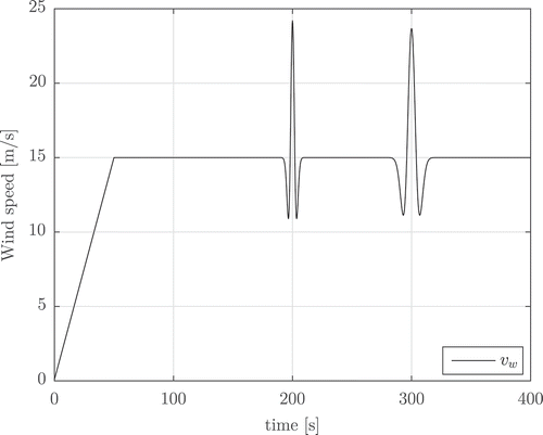
To verify the controller performance, eight different scenarios (cases) have been simulated for which the wind speed trajectory is varied:

• Wind ramps with different constant end wind speed $v_{w,\mathrm{m}\mathrm{a}\mathrm{x}}$ (11,12,15,18 and 22 m/s).

• Linear wind speed slope from 0 to 30 m/s.

• Wind ramp with single wavelet disturbance.

• Wind ramp with double wavelet disturbances.

The different cases are used to test different conditions for the control system of the wind turbine. The first five cases with the wind ramps are used to simulate the nominal conditions for the controller with constant wind speed after a transient startup phase. For these cases no major improvements can be expected compared to the reference controller. However these cases are important, since the advanced control system should also perform well in nominal conditions, and not only focus on load reduction.

The linear wind speed slope is used to verify the transition phases for the control law. For example the pitch control and pitch feed-forward control are only active if the generator speed is close to its allowed maximum ${\omega }_{g,high}$ and also the scheduled PI-Pitch controller has different gains depending on the current pitch angle $\gamma$. In addition the set point ${\lambda }_r$ for the NDI control loop changes based on the current wind speed $v_w$.

The last two cases are used to simulate the controller behaviour under gust load conditions. To simulate the wind gust excitation of the elastic wind turbine tower, Ricker wavelets according to Equation (17) are used. The wavelets are parameterized to simulate short wind gusts (see Figure 12):

(17) $\psi (t)=\frac{2}{\sqrt{3\sigma }{\pi }^{\frac{1}{4}}}\left(1-\frac{t^2}{{\sigma }^2}\right)e^{\frac{-t^2}{2{\sigma }^2}}.$(17)

Figure 12. Wind speed for the scenario with a wind ramp and double wavelet disturbances.

Two criteria have been defined for the simulated scenarios to quantify the generated energy of the turbine and the load of the wind turbine tower in Equation (13):

(18a) $C_a={\int }_0^{400}|a_t{|}_{1}dt,$(18a)

(18b) $C_p={\int }_0^{400}{\tau }_g{\omega }_{g}dt.$(18b)

The criteria $C_a$ is a measure for the load and is computed from the integral over the simulation time of 400 s of the L1 norm of the acceleration $a_t$ at the tip of the tower. A reduction of $a_t$ is desirable to prolong the turbine’s lifetime. The second criteria $C_p$ is the generated energy of the wind turbine during the simulation. An increase in $C_p$ leads to a more efficient turbine. Figure 13 gives an overview of the results that have been normalized to the maximum values of all cases. As can be seen from the plot, the generated energy is very similar for all cases for the reference controller and the NDI based control system. Using the wind speed measurement, the NDI controller is able to react faster what leads to a slight increase in generated energy. However the main added benefit from the advanced control law based on the wind measurement can be seen for the resulting acceleration at the tower tip during gust loads.

Figure 13. Normalized results of the generated energy of the wind turbine and acceleration at the tower tip for the different simulated scenarios.

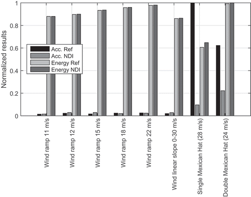
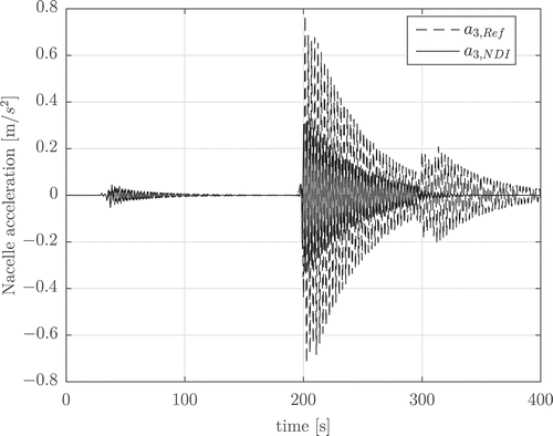
The wind gust, simulated by the wavelets, leads to very strong acceleration at the tower tip that can be reduced substantially using the new proposed control system, as can be seen in Figure 8. In particular, for the case with only one wind gust peak, the wind gust load can be absorbed directly using the NDI control law of the generator.

Figure 14 shows the resulting generator torque for this scenario, Figure 15 the corresponding generator speed, Figure 12 the wind speed and Figure 16 the rotor pitch angle. As can be seen from the plots, the new generator controller is able to use the additional information from the measured wind speed to react faster to changes in the wind speed, which results in a much smoother generator speed and generator torque for the NDI controller and additionally reduces the acceleration at the tower tip, as can be seen in Figure 17. In addition the feed-forward control law for the rotor pitch angle leads to a faster response. The reduced acceleration also lessens the load on the tower structure.

Figure 14. Comparison of the resulting generator torque for the scenario with a wind ramp and double wavelet disturbances.

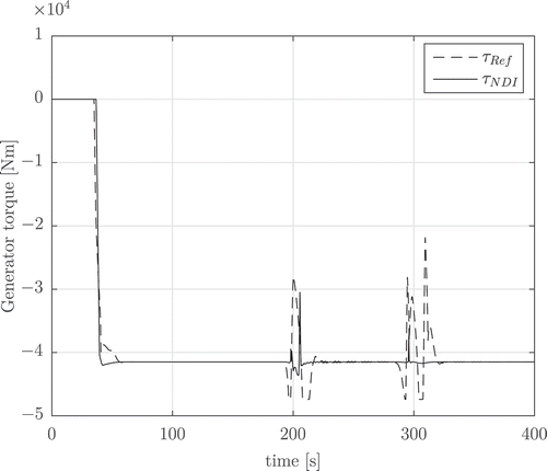
Figure 15. Comparison of the resulting generator speed for the scenario with a wind ramp and double wavelet disturbances.

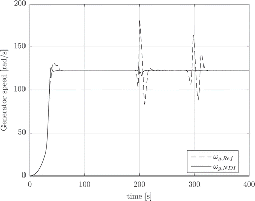
Figure 16. Rotor pitch angle comparison for the scenario with a wind ramp and double wavelet disturbances.

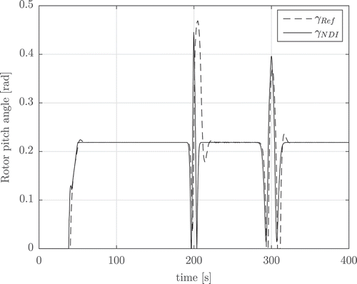
Figure 17. Acceleration vector component parallel to the wind direction at the top of the tower for the double wavelet scenario.

The developed controller serves as an application example for the newly developed Modelica library which can make use of powerful features like automatic inversion. However for an implementation on a real wind turbine further analysis and investigations would have to be performed. To achieve a better robustness analysis a full lifetime analysis with turbulent 3D wind fields and the inclusion of the LIDAR-based wind speed estimation should be considered, however this was outside the scope of our current project, where the main focus was the development of an extensive and unified modelling library for wind turbines.

6. Conclusion and future work

The current design of controllers for wind turbines is rather conservative. The results of the last chapters indicate that using advanced control methods such as NDI, significant performance gains can be achieved especially in the field of load mitigation. LIDAR systems, however, are a key technology to enable the described control method. We expect LIDAR systems to become more widespread among new or retrofitted wind turbines due to upcoming reductions in production cost, especially in wind farms where one LIDAR system can be used for multiple turbines.

Modern control methods such as NDI represent model-based approaches. A multi-domain Modelica library for wind turbines with non-causal and hence invertible models forms an optimal basis for the development of suitable NDI controllers.

Whereas table-based approaches for aerodynamic efficiency form the basis of the nonlinear controller design, more detailed models of the aeroelastic behaviour of a wind-turbine can be used for virtual testing. Building upon existing components for flexible and rigid bodies and creating a robust model component for blade elements, together enables the simulation of a complete wind power plant. The desired level of detail can thereby be chosen by the modeller, and the models are versatile for their use in various studies.

In particular, the simulation results for the NDI & PCH based controller, using advanced capabilities of Modelica and FMI, shows promising results. Using the newly developed object oriented Modelica modelling library allows to obtain inverse models of the wind turbine easily and therefore allows to implement the NDI control laws in a very straightforward manner. However in the future it would be necessary to verify the control systems on real wind turbines to analyse the robustness and performance under realistic conditions.

We hope that the simulation-based analysis can help to motivate the use of advanced control systems and sensors in the future. The presented object-oriented models in Modelica form a well-suited basis for such tasks. The modularity and multi-domain approach make their use also attractive for future applications regarding net integration or the optimized operation of wind farms.

Acknowledgements

The development of Modelica models for wind turbines is supported by DLR Technology Marketing. The authors thank Daniel Milz for his help with the illustration work.

Disclosure statement

No potential conflict of interest was reported by the authors.

Additional information

Funding

The development of Modelica models for wind turbines is supported by DLR Technology Marketing.

Notes

1. German Aerospace Center (German: Deutsches Zentrum für Luft- und Raumfahrt).

References

- Modelica Association, editor. Modelica - A Unified Object-Oriented Language for Physical Systems Modeling Language Specification Version 3.2,Como.Linköping: Linköping University Press, 2010.
- T. Bellmann, Interactive simulations and advanced visualization with modelica, Proceedings of the 7th Modelica Conference, 541–550, 2009.
- FMI development group, Functional mock-up interface for model exchange and co-simulation. Technical report, MODELISAR consortium, 2014.
- J. Jonkman, S. Butterfield, W. Musial, and G. Scott, Definition of a 5-mw reference wind turbine for offshore system development. Technical report, National Renewable Energy Laboratory, 2009.
- J. Tobolar, M. Otter, and T. Bünte, Modelling of vehicle powertrains with the modelica powertrain library, in Systemanalyse in Der Kfz-Antriebstechnik IV, Systemanalyse in der Kfz-Antriebstechnik IV”, Essen, Germany, 2007.
- G. Looye, The new DLR flight dynamics library, Proceedings of the 6th Modelica Conference, 193–202, 2008.
- A. Heckmann, M. Otter, S. Dietz, and J. Lopez, The DLR Flexible Bodies Library to Model Large Motions of Beams and of Flexible Bodies Exported from Finite Element Programs, The Modelica Association, Linköping University Press, Linköping 2006.
- M. Hansen, Aerodynamics of Wind Turbines, Earthscan, Routledge, London, 2008.
- O. Wallrapp, Standardization of flexible body modeling in multibody system codes, part I: definition of standart input data, Mech. Struct. Mach. 22 (3) (1994), pp. 283–304. doi:10.1080/08905459408905214
- P. Thomas, X. Gu, R. Samlaus, C. Hillmann, and U. Wihlfahrt, The onewind modelica library for wind turbine simulation with flexible structure - modal reduction method in modelica, Proceedings of the 10th International Modelica Conference, 2014.
- A. Craig Hansen and P.J. Moriarty. Aerodyn theory manual, Technical report, National Renewable Energy Laboratory, 2005.
- J. Twele and R. Gasch, Windkraftanlagen, Vieweg+Teubner, Wiesbaden, Germany, 2011.
- D. Zimmer. Using artificial states in modeling dynamic systems: turning malpractice into good practice, Proceedings of the 5th International Workshop on Equation-Based Object-Oriented Languages and Tools (EOOLT), 2013.
- M. Otter, H. Elmqvist, and S. Mattsson, The new modelica multibody library, Proceedings of the 3rd International Modelica Conference, 2003.
- F. Dunne, E. Simley, and L. Pao, Lidar wind speed measurement analysis and feed-forward blade pitch control for load mitigation in wind turbines. Technical report, National Renewable Energy Laboratory, 2011.
- A. Koerber and R. King, Combined feedback–feedforward control of wind turbines using state-constrained model predictive control, Ieee. Trans. Control. Syst. Technol. 21 (4) (2013), pp. 1117–1128. doi:10.1109/TCST.2013.2260749
- D. Schlipf, T. Fischer, C. Carcangiu, M. Rossetti, and E. Bossanyi. Load analysis of look-ahead collective pitch control using lidar, Proceedings of the 10th German Wind Energy Conference DEWEK, 17-18 Nov 2010. Universität Stuttgart, 2010.
- N. Wang and K. Johnson, Lidar-based fx-rls feedforward control for wind turbine load mitigation, Proceedings of the 2011 American Control Conference, 2011.
- J.-J.E. Slotine and L. Weiping, Applied Nonlinear Control, Pearson, Upper Saddle River, NJ, 1991.
- E. Johnson and A. Calise, Pseudo-Control Hedging: A New Method for Adaptive Control,Workshop on Advances in Guidance and Control Technology, Alabama, USA, 2000.
- H. Geng, S. Xiao, W. Yang, and G. Yang. Nonlinear dynamic inversion approach applied to pitch control of wind turbines, Proceeding of the 11th World Congress on Intelligent Control and Automation, 2014.
- F. Holzapfel, Nichtlineare adaptive regelung eines unbemannten fluggerätes, Verlag Dr. Hut.Ph. D. Thesis, Technische Universität München, München, (2004).
- T. Lombaerts, G. Looye, Q. Chu, and J. Mulder, Design and simulation of fault tolerant flight control based on a physical approach, Aerospace Sci. Technol. 23 (1) 35th ERF: Progress in Rotorcraft Research (2012), pp. 151–171. doi:10.1016/j.ast.2011.07.004.
- G. Looye, Design of robust autopilot control laws with nonlinear dynamic inversion, Automatisierungstechnik. 49 (2001), pp. 523–531. doi:10.1524/auto.2001.49.12.523
- L.Y. Eric Simley, N.K. Pao, B. Jonkman, and R. Frehlich, Lidar wind speed measurements of evolving wind fields, Proc. ASME Wind Energy Symposium, 2012.
- L.Y. Fiona Dunne, D.S. Pao, and A.K. Scholbrock, Importance of lidar measurement timing accuracy for wind turbine control, American Control Conference, ACC 2014, Portland, OR, USA, June 4-6, 2014, 3716–3721, 2014.
- D. Schlipf and P.-W. Cheng, Adaptive vorsteuerung für windenergieanlagen, Automatisierungstechnik. 61 (5) (2013), pp. 329–338. doi:10.1524/auto.2013.0029
- E. Bossanyi, B. Savini, M. Iribas, M. Hau, B. Fischer, D. Schlipf, T. van Engelen, M. Rossetti, and C.E. Carcangiu, Advanced controller research for multi-mw wind turbines in the upwind project, Wind Energy. 15 (1) (2012), pp. 119–145. doi:10.1002/we.v15.1
- S. Mattsson and G. Söderlind, Index reduction in differential-algebraic equations using dummy derivatives, SIAM J. Scientific Stat. Comput. 14 (1993), pp. 677–692. doi:10.1137/0914043
- M. Otter, H. Elmqvist, and F. Cellier. Modeling of multibody systems with the object-oriented modeling language dymola, Technical report, 1996.
- M. Reiner. Modellierung und Steuerung eines strukturelastischen Roboters. PhD thesis, Technische Universität München, 2011.
- H. Joos, J. Bals, G. Looye, K. Schnepper, and A. Varga. A multi-objective optimisation based software environment for control systems design. Proc. of 2002 IEEE International Conference on Control Applications and International Symposium on Computer Aided Control Systems Design, CCA/CACSD, 2002.
- M. Reiner and D. Zimmer. Nonlinear dynamic inversion control for wind turbine load mitigation based on wind speed measurement. In Proceedings of the 11th International Modelica Conference, 349–357, 2015.