On the evaluation of the takeoff time and of the peak time for innovation diffusion on assortative networks

ABSTRACT

This paper deals with a generalization of the Bass model for the description of the diffusion of innovations. The generalization keeps into account heterogeneity of the interactions of the consumers and is expressed by a system of several nonlinear differential equations on complex networks. The following contributions can be singled out: first, explicit algorithms are provided for the construction of various families of assortative scale-free networks; second, a method is provided for the identification of the takeoff time and of the peak time, which represent important turning points in the life cycle of an innovation/product; third, the emergence of specific patterns in connection with networks of the same family is observed, whose tentative interpretation is then given. Also, a comparison with an alternative approach is given, within which adoption times of different communities are evaluated of a network describing firm cooperations in South Tyrol.

KEYWORDS:

• Innovation diffusion
• Bass model
• assortative networks
• takeoff and peak time

1. Introduction

The findings described in this paper are related to the identification of the time at which the adoption rate of new products in a community of variously interconnected individuals reaches its maximum and of the takeoff time, another quantity of interest in the marketing perspective. The investigation of this problem is carried out here within a framework which extends on complex networks the classical Bass model.

Since its first appearance in the Sixties, the Bass model [1] for the description of the innovation diffusion process has been extensively applied (the reviews [2] and [3] provide several references in this connection). Also, during the course of time, several versions of this model have been formulated, which provide generalizations in a variety of directions (see, e.g. [4,5]). The original version is expressed by a single ordinary differential equation, in fact a Riccati one, which is, albeit non-linear, analytically solvable. Its solution describes the evolution in time of the number of adopters of new products within a population, as a consequence of two basic factors, innovation and imitation. An aggregate perspective is taken, in that only the cumulative fraction of adopters is considered and, for a fixed product, the two parameters appearing in the equation, the ‘innovation’ and the ‘imitation’ coefficient, are the same for the whole population.

It is, however, to be expected that a thorough investigation keeps into account heterogeneity of the individuals. This can be done in different ways, among whose a significant one is to consider the network of interpersonal connections. Indeed, especially in regard to the imitation aspect of the process, it can make a big difference whether individuals who have already adopted have a few or several contacts [6]. Driven by this motivation, we have introduced in [7,8] a network structure into the model. Specifically, we have considered networks whose nodes have at most a fixed number $n$ of links. A first statistical attribute of networks is given by the so-called degree distribution $P(k)$, which carries information on the fraction of nodes having $k$ links. Further and central importance in relation to the network topology have the degree correlations $P(h|k)$, with $P(h|k)$ expressing the conditional probability that an individual with $k$ links is connected to one with $h$ links. In [7,8], following the approach developed for the study of epidemic spreading on complex networks [9–11], we have reformulated the Bass equation

(1) $\frac{dF(t)}{dt}=[1-F(t)]\left[p+qF(t)\right]$(1)

(in which $F(t)$ is the cumulative adopter fraction at the time $t$, and $p$ and $q$ are the innovation and the imitation coefficient, respectively) into a system of $n$ ordinary differential equations, one for each admissible number of links, of the form

(2) $\frac{d{G}_j(t)}{dt}=[1-G_j(t)]\left[p+jq\sum _{h=1}^{n}P(h|j)G_h(t)\right]j=1,...,n.$(2)

The quantity $G_j(t)$ in (2) represents for any $j=1,...n$ the fraction of potential adopters with $j$ links that at the time $t$ have adopted the innovation. More precisely, denoting by $F_j(t)$ the fraction of the total population composed by individuals with $j$ links, who at the time $t$ have adopted, and admitting that, in the end, all individuals will adopt (in analogy with the fact that the solution $F(t)$ of (1) tends to $1$ as $t$ tends to infinity), we set $G_j(t)=F_j(t)/P(j)$.

In principle, one could consider at this point different kinds of networks. We dealt with scale-free ones, having degree distribution of the form $P(k)=c/k^{\gamma }$ where $2<\gamma <3$, because it is into this category and with power-law exponent into this range that many real-world networks fall [12,13]. We explored various features of the different link classes for both correlated and uncorrelated networks, comparing results of numerical simulations relative to system (2) with results relative to Equation (1). In particular, to perform this task, we devised an algorithm for the construction of both assortative and disassortative networks.

In this paper, in view of the foreseen application and of the fact that networks in the social sciences are found to be typically assortative [14,15], we further restrict attention to their category. Yet, we observe en passant that in the modelling of diffusion and innovation also networks falling beyond the group of the social ones, notably collaboration networks among firms, may play a part. And in fact, we deal with such a network, disassortative indeed, in Section 5, where an approach alternative to that one based on Equation (2) is discussed.

It is now worth recalling that some procedures designed to construct correlated networks, in fact, exist in the literature. For instance [16], and [17] suggest different rewiring-based algorithms which generate assortatively mixed networks and assortative mixing to a desired degree; in [18] a network model which encompasses addition of both new nodes and new links, meant to mimic a real growing network (a preprint-archive) is introduced; besides [19], and [20] propose models for (assortative and disassortative) complex networks with weighted links. However, precise explicit (not only approximate) expressions for the correlations $P(h|j)$, suitable to be employed in calculations, can be hardly found in these or other papers. And the numerical solutions of our differential Equation (2) require the knowledge of a set of values of $P(h|j)$ defined for each $h$ and $j$ and satisfying as well suitable conditions of normalization and network closure, see Section 2. For this reason, we start providing in the next section a few ‘recipes’ towards building correlation matrices of assortative networks. In Section 3 we focus on the identification in the present analytical context of two specific times (takeoff time and peak time) which play a significant role in the life cycle of an innovation/product. Then, we calculate these times for several networks belonging to the families devised in Section 2. A comparison between the degree correlation matrices pertaining to different networks of the same family for each of three families reveals the existence of unexpected patterns, which call for explanation. This is the subject of Section 4, where also a possible interpretation is proposed. Elements of an approach alternative to that based on a mean-field approximation dealt with in Sections 2–4 are discussed in Section 5. In that section also the calculation is done of adoption times of different communities in a network model of firms in South Tyrol. We want to stress however that the purpose of this paper is to construct an analytical framework for the evaluation of the mentioned times, rather than to treat experimental data. Finally, in Section 6, a summary of the results and our conclusions are given.

It may be of interest before continuing to point out how lively and vivid the interest in innovation dynamics and spreading phenomena still is. As the following few but indicative recent references show, research related to these topics keeps growing and branching out into a manifold of novel paths. For example, an agent-based model for the description of the Skype technology large-scale adoption process is proposed in [21]. An analysis and a discussion of the diverse roles of rational strategic approaches and serendipity towards the development of innovations are carried out in [22]. An evolutionary game model with interacting innovators and developers is suggested in [23] to investigate to which extent a system is able to maintain innovators. In [24] a model for the emergence of innovations is devised which involves random walks on networks whose nodes represent concepts and ideas. A simple model, inspired by the Lotka-Volterra one regarding competition for common resources occurring among species is employed in [25] to ‘measure the pace’ of collective attention through the inflationary information flows of popular topics and cultural items. Further articles on the subject can be found in the collection [26].

2. Families of assortative networks

We start here by suggesting a practical way for the construction of different families of assortative networks (namely, such that high degree nodes tend to be linked to other high degree nodes, whereas low degree nodes tend to be linked to other low degree nodes). We consider for any fixed natural number $n$ a scale-free network with degree distribution $P(k)=c/k^{\gamma }$ for $k\le n$ ($k\ge 1$), with $2<\gamma <3$. We aim at building the $n\times n$ matrices, whose elements are the correlation coefficients $P(h|k)$. The reason why this is a delicate task is that the $P(k)$ and $P(h|k)$ must satisfy, besides the normalizations

$\sum _{k=1}^{n}P(k)=1,\mathrm{a}\mathrm{n}\mathrm{d}\sum _{k=1}^{n}P(h|k)=1,$

and the positivity requirements

$P(k)\ge 0,\mathrm{a}\mathrm{n}\mathrm{d}P(h|k)\ge 0,$

also the Network Closure Condition (NCC)

(3) $hP(k|h)P(h)=kP(h|k)P(k),\mathrm{\forall }h,k=i=1,...,n.$(3)

We recall here that the assortativity of a network can be established by looking at the average nearest neighbour degree function

(4) $k_{nn}(k)=\sum _{h=1}^{n}hP(h|k).$(4)

Indeed, if $k_{nn}(k)$ is increasing in $k$, the network is assortative. Alternatively, one can calculate the Newman assortativity coefficient $r$ (Pearson correlation coefficient) as defined in [14] (see also [27]).

We propose next the construction of three different matrices (in fact, matrix families), starting from a first requirement that their largest elements are on the diagonal, whereas their other elements become smaller and smaller the more apart from the diagonal they are. Notice first that the NCC condition (3) provides a constraint on the correlation matrix elements expressed by

(5) $P(h|k)=P(k|h)\frac{h^{1-\gamma }}{k^{1-\gamma }}.$(5)

$\bullet$ ‘Power-like’ family. A first natural choice is that of taking the elements on and above the diagonal as

(6) $P(h|k)=\left\{\begin{array}{c}|h-k{|}^{-\lambda }\mathrm{i}\mathrm{f}h<k\\ 1\mathrm{i}\mathrm{f}h=k\end{array}\right.$(6)

for some $\lambda >0$, and the elements under the diagonal, i.e. with $h>k$, defined through the formula (5).

Since the normalization ${\sum }_{k=1}^{n}P(h|k)=1$ has to hold true, we compute for any $k=1,...,n$ the sum $C_k={\sum }_{h=1}^{n}P(h|k)$ and call $C_{max}$ the greatest of these sums:

$C_{max}=\underset{k=1,\dots ,n}{max}{C}_k.$

At this point, we re-define the correlation matrix by setting the elements on the diagonal equal to

$P^{\prime }(k|k)=C_{max}-C_k,k=1,\dots ,n,$

and leaving the other elements unchanged. For any $k=1,...,n$ the column sum ${\sum }_{h=1}^n{P}^{\prime }(h|k)$ is then equal to

$C_k^{\prime }=C_k-1+C_{max}-C_k=C_{max}-1.$

Finally, we normalize the entire matrix by setting

$P^{\prime \prime }(h|k)=\frac{1}{(C_{max}-1)}{P}^{\prime }(h|k),h,k=1,\dots ,n.$

A number of numerical simulations in correspondence to different values of $n$ and $\lambda$ show that the function

(7) $k_{nn}(k)=\sum _{h=1}^{n}h{P}^{\prime \prime }(h|k)$(7)

is increasing. A graphical representation (for the case in which $n=99$, $\gamma =2.5$ and $\lambda =1$) is given in the left panel of Figure 1. We then conclude that these correlation matrices define a one-parameter family ($\lambda$ being the parameter) of assortative networks.

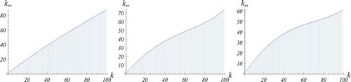
Figure 1. The three panels in this figure display the increasing character of the function $k_{nn}(k)$ for networks of the three families introduced in this section. Specifically, the left panel refers to a network of the power-like family, the central panel refers to a network of the linear family, and the right panel refers to a network of the exponential family. In all cases, the maximum number $n$ of links of the network is equal to $99$, the parameter $\gamma$ (the exponent of the power-law degree distribution) is equal to $2.5$ Also, the parameters $\lambda ,\mu$ and $\nu$ are all equal to $1$.

$\bullet$ ‘Linear’ family. Another possibility is to start by defining, for $\mu \in (0,1]$, the elements on and above the diagonal as

(8) $P(h|k)=1-\frac{\mu }{N}|h-k|\mathrm{i}\mathrm{f}h\le k$(8)

and the elements under the diagonal as in the formula (5).

To get the normalization ${\sum }_{k=1}^{n}P(h|k)=1$, one can then apply the same procedure as for the first network family. In this case too, $k_{nn}(k)$ turns out to be increasing in $k$ suggesting assortativity for the $\mu$ family of networks with correlations $P^{\prime \prime }(h|k)$. A graphical representation of the increasing character of $k_{nn}(k)$ (for the case in which $n=99$, $\gamma =2.5$ and $\mu =1$) is given in the central panel of Figure 1.

$\bullet$ ‘Exponential’ family. A further possibility is to start by defining the elements on and above the diagonal as

(9) $P(h|k)=e^{-\nu \frac{{(h-k)}^2}{n^2}}\mathrm{i}\mathrm{f}h\le k$(9)

and the elements under the diagonal as in the formula (5).

Once again, the adjustment procedure necessary to get the required normalization is as for the two previous network families. And again, the increasing character of $k_{nn}(k)$, displayed as a result of a large number of simulations, supports the assortativity of the networks associated to these correlation matrices. The increasing character of $k_{nn}(k)$ (for the case in which $n=99$, $\gamma =2.5$ and $\nu =1$) is given in the right panel of Figure 1.

2.1. Alternative assortative matrices

We briefly outline here an alternative possibility for the construction of assortative networks. It consists in starting by assigning symmetrical correlation matrices of the ‘$e_{jk}$’ type (excess-degree correlations, with $j,k=0,\dots ,n-1$, see [12,13]) with larger correlation for similar degree, and derive from them the excess-degree distribution $q_k$ as $q_k={\sum }_{j=0}^{n-1}{e}_{jk}$ and the degree distribution $P(k)$ as $P(k)=\frac{k^{-1}{q}_{k-1}}{{\sum }_{j=1}^n{j}^{-1}{q}_{j-1}}$. With suitable choices of $e_{jk}$ one can obtain, in this way, a degree distribution which is well approximated by a power law. The disadvantage of this procedure is that the degree distribution is not obtained in general in explicit form, but as the sum of a series. Still, this technique can be useful in order to enlarge the choice of the possible assortative correlations.

We recall the relations between $P(k)$, $P(h|k)$ and $q_k$, $e_{jk}$:

(10) $P(h|k)=\frac{{\tilde{e}}_{kh}}{{\sum }_{j=1}^n{\tilde{e}}_{kj}}\mathrm{\forall }h,k=i=1,...,n;$(10)

(11) ${\tilde{e}}_{hk}=\frac{P(h|k)kP(k)}{{\sum }_{j=1}^{n}jP(j)},$(11)

where ${\tilde{e}}_{k,h}=e_{k-1,h-1}$. By definition, $e_{jk}$ is the fraction of links in the network joining nodes of excess degrees $j$ and $k$. Therefore, it is always symmetrical. This implies that any set of $P(k)$, $P(h|k)$ obtained from a given $e_{jk}$ automatically satisfy the Network Closure Condition.

As a simple example consider

(12) $e_{jk}=c_{\delta }\frac{1}{{(1+j+k)}^{\delta }},$(12)

where $c_{\delta }$ is a normalization constant depending on $\delta$ and determined from the condition ${\sum }_{j,k=0}^{n-1}{e}_{jk}=1$. 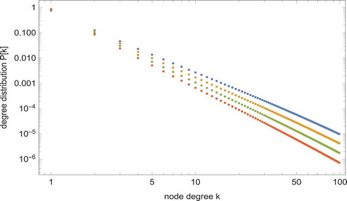Taking for instance $\delta =2.2$, $\delta =2.4$, $\delta =2.6$ and $\delta =2.8$ respectively for a network with $n=99$, we obtain Newman assortativity coefficients $r=0.51$, $r=0.53$, $r=0.53$ and $r=0.53$ and degree distributions $P(k)$ behaving as $c/k^{\gamma }$ with $\gamma =2.42$, $\gamma =2.61$, $\gamma =2.79$ and $\gamma =2.98$ respectively¹. Figure 2 shows the log-log plots of these degree distributions.

Figure 2. Log-log plots of the degree distributions obtained for networks with $n=99$ by assigning excess-degree correlations $e_{jk}=c_{\delta }/(1+j+k{)}^{\delta }$, with $\delta =2.2$, $\delta =2.4$, $\delta =2.6$ and $\delta =2.8$. The plots are ordered from the upper one ($\delta =2.2$) to the lower one ($\delta =2.8$). The degree distributions $P(k)$ behave as $c/k^{\gamma }$ with $\gamma =2.42$, $\gamma =2.61$, $\gamma =2.79$ and $\gamma =2.98$ respectively.

The assortativity of these networks is also evident from the increasing character of their average nearest neighbour degree functions $k_{nn}(k)$. In Figure 3 those corresponding to $\delta =2.2$ and $\delta =2.8$ are displayed.

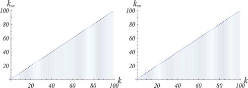
Figure 3. The two panels show the increasing character of the function $k_{nn}(k)$ for two networks with a maximum number $n$ of links equal to $99$ and excess-degree correlations as in (12) with $\delta =2.2$ (left panel) and $\delta =2.8$ (right panel).

3. Looking for the adoption peak time

An issue of considerable interest in connection with the diffusion of innovations is the identification of the peak time, which is the time corresponding to the peak of sales in marketing applications. To be more concrete, let $f_j(t)={\dot{F}}_j(t)$, where $F_j(t)$ is as in the Introduction and the dot denotes the time derivative, denote the fraction of new adoptions per unit time in the ‘link class $j$’ i.e. in the subset of individuals having $j$ links. And let $f(t)=\sum _{i=1}^n{f}_j(t)$ be the total number of new adoptions per unit time. The three panels in Figure 4 help to illustrate the concept. The left panel displays the evolution in time of the population fractions $F_j(t)$ for $j=1,...,9$. To fix ideas, an underlying network of the first family with parameters $n=9$, $\gamma =2.9$ and $\lambda =1$ has been chosen. The innovation and the imitation coefficients $p$ and $q$ are taken to be equal to $0.03$ and $0.4$, respectively, which are conceivable values employed in the traditional literature on the Bass equation². The centre panel shows the evolution in time of the nine functions $f_j(t)$, whereas the right panel displays the evolution in time of the function $f(t)=\sum _{i=1}^n{f}_j(t)$, together with that one of the function $\dot{F}(t)$ relative to the original Bass equation. 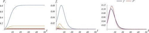The values of $t$ in correspondence to which the two graphs have a maximum are the peak time of the system on the network (occurring a little bit earlier) and the one of the homogeneous Bass system (occurring a little bit later on) respectively.

Figure 4. The left panel displays the evolution in time of the population fractions $F_j(t)$ in the case of an underlying network of the ‘power-like’ family with parameters $n=9$, $\gamma =2.9$ and $\lambda =1$. The innovation coefficient $p$ is equal to $0.03$ and the imitation coefficient $q$ is equal to $0.4$. The graphs of the functions $F_j$, as in the centre panel those of the functions $f_j$, are ordered from the upper one ($j=1$) to the lower one ($j=9$). One may observe that the largest fraction of new adopters belongs at all times to a single link class, the link class with $j=1$, which reaches its adoption peak later than the others. The fact that more connected individuals adopt earlier is a general (and rather intuitive) phenomenon. The centre panel shows the evolution in time of the nine functions $f_j(t)$, whereas the right panel displays the evolution in time of the function $f(t)$ together with that of the function $\dot{F}(t)$ relative to the original Bass equation. The values of $t$ in correspondence to which the two graphs have a maximum are the peak time of the system on the network and of the homogeneous Bass system, respectively.

Another time value of interest, especially for industry analysts, for managers and firms producing the innovations, is the so-called takeoff time, which represents the moment when a transition from the initial phase to a growth phase occurs. This time can be found in the context of the generalized Bass model on networks as the time at which the acceleration of the function $F_{net}(t)=\sum _{i=1}^n{F}_j(t)$ (which expresses the fraction at time $t$ of the population which has adopted) is maximal and, hence, the third derivative of $F_{net}(t)$ vanishes. Equivalently, at this point, the second derivative of $f(t)=\sum _{i=1}^n{f}_j(t)$ vanishes and the graph of $f(t)$ has an inflection point. Hence, this time also marks the point when, even if sales continue to increase, their increase increment begins diminishing. 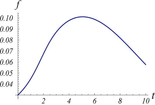A portion of the graph of the function $f(t)$ appearing in Figure 4 is displayed in Figure 5 where times have been scaled so as to make evident the existence of an inflection and of a maximum point.

Figure 5. A portion of the graph of the function $f(t)$ of Figure 4 is here displayed with time scaling suitable to make evident the existence of an inflection point (the takeoff point) and of a maximum point (the peak point).

We calculated both the takeoff and the peak time for several networks belonging to three families of Section 2. Results relative to a sample of networks for each family are reported in the three Tables 1, 2 and 3. There, a specific network is identified by the values of the two parameters $\gamma$ and $\lambda$ in the case of the ‘power-like’ family, $\gamma$ and $\mu$ in the case of the ‘linear’ family, $\gamma$ and $\nu$ in the case of the ‘exponential’ family. Notice that in the three tables for each network also the assortativity coefficient $r$ is calculated. Also, to improve the readability of the results contained in the tables, Figure 6 is here inserted. The two panels in this figure display two surfaces, respectively, obtained through interpolation of the values of the takeoff time and of the peak time for the ‘power-like’ family in correspondence to the values of the parameters $\gamma$ and $\lambda$ mentioned in Table 1. Similar figures for the other two families are qualitatively similar and hence are not reported here.

Figure 6. The panels display two surfaces, respectively, obtained through interpolation of the values of the takeoff time (left panel) and of the peak time (right panel) for the ‘power-like’ family in correspondence to the values of the parameters $\gamma$ and $\lambda$ mentioned in Table 1. Similar figures for the other two families are qualitatively similar and hence are not reported here.

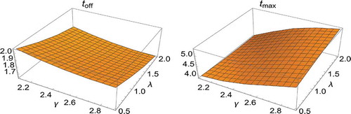
Table 1. This table provides approximate values for the takeoff time, the peak time and the assortativity coefficient of 20 networks of the ‘power-like’ family in Section 2.

‘Power-like’ family	$\lambda =0.5$	$\lambda =1.0$	$\lambda =1.5$	$\lambda =2.0$
takeoff time $t_{off}$
$\gamma =2.1$	2.049	1.934	1.843	1.783
$\gamma =2.3$	1.994	1.879	1.786	1.723
$\gamma =2.5$	1.955	1.838	1.744	1.678
$\gamma =2.7$	1.932	1.814	1.717	1.650
$\gamma =2.9$	1.925	1.807	1.708	1.638
peak time $t_{max}$
$\gamma =2.1$	3.967	3.907	3.891	3.903
$\gamma =2.3$	4.060	4.116	4.244	4.386
$\gamma =2.5$	4.277	4.454	4.655	4.816
$\gamma =2.7$	4.585	4.794	4.975	5.108
$\gamma =2.9$	4.891	5.064	5.205	5.307
assortativity coefficient $r$
$\gamma =2.1$	0.594	0.716	0.803	0.857
$\gamma =2.3$	0.626	0.734	0.811	0.861
$\gamma =2.5$	0.652	0.748	0.817	0.863
$\gamma =2.7$	0.673	0.759	0.821	0.863
$\gamma =2.9$	0.690	0.767	0.823	0.861

Table 2. This table provides approximate values for the takeoff time, the peak time and the assortativity coefficient of 20 networks of the ‘linear’ family in Section 2.

‘Linear’ family	$\mu =0.25$	$\mu =0.5$	$\mu =0.75$	$\mu =1.0$
takeoff time $t_{off}$
$\gamma =2.1$	2.136	2.113	2.075	2.017
$\gamma =2.3$	2.080	2.059	2.021	1.967
$\gamma =2.5$	2.040	2.020	1.984	1.931
$\gamma =2.7$	2.013	1.995	1.961	1.910
$\gamma =2.9$	2.002	1.985	1.955	1.905
peak time $t_{max}$
$\gamma =2.1$	4.037	4.020	3.992	3.959
$\gamma =2.3$	4.069	4.069	4.065	4.075
$\gamma =2.5$	4.200	4.219	4.248	4.302
$\gamma =2.7$	4.443	4.476	4.525	4.598
$\gamma =2.9$	4.749	4.781	4.824	4.885
assortativity coefficient $r$
$\gamma =2.1$	0.481	0.513	0.563	0.629
$\gamma =2.3$	0.530	0.555	0.598	0.654
$\gamma =2.5$	0.570	0.590	0.627	0.674
$\gamma =2.7$	0.602	0.620	0.650	0.691
$\gamma =2.9$	0.629	0.644	0.668	0.705

Table 3. This table provides approximate values for the takeoff time, the peak time and the assortativity coefficient of 20 networks of the ‘exponential’ family in Section 2.

‘Exponential’ family	$\nu =0.5$	$\nu =1.0$	$\nu =1.5$	$\nu =2.0$
takeoff time $t_{off}$
$\gamma =2.1$	2.128	2.096	2.067	2.036
$\gamma =2.3$	2.073	2.043	2.014	1.987
$\gamma =2.5$	2.033	2.006	1.976	1.949
$\gamma =2.7$	2.007	1.984	1.955	1.928
$\gamma =2.9$	1.997	1.977	1.949	1.924
peak time $t_{max}$
$\gamma =2.1$	4.032	4.008	3.989	3.970
$\gamma =2.3$	4.070	4.067	4.068	4.073
$\gamma =2.5$	4.208	4.229	4.255	4.284
$\gamma =2.7$	4.454	4.492	4.532	4.572
$\gamma =2.9$	4.758	4.791	4.827	4.861
assortativity coefficient $r$
$\gamma =2.1$	0.492	0.535	0.572	0.608
$\gamma =2.3$	0.539	0.574	0.606	0.635
$\gamma =2.5$	0.578	0.605	0.634	0.658
$\gamma =2.7$	0.609	0.631	0.656	0.677
$\gamma =2.9$	0.634	0.651	0.673	0.692

4. Emerging patterns

The patterns announced in the Introduction come out as follows: If one fixes a value of the parameter $\lambda$ or $\mu$ or $\nu$, depending on which of the three tables relative to the three network families she is considering, it is immediate to check that the peak times increase as the parameter $\gamma$ increases passing from $2.1$ to $2.9$. As well, the takeoff times diminish as $\gamma$ increases. It is then tempting to try and compare the degree correlation matrices pertaining to networks with different values of $\gamma$. Somehow surprisingly, it turns out that each time one subtracts the degree correlation matrix of a network with a certain $\gamma$ from the degree correlation matrix of a network with a greater $\gamma$ (keeping the other parameter fixed) one gets a matrix for which all entries below the main diagonal are negative, whereas all elements above the main diagonal are positive. For example, the difference $P_{(\mu =0.5,\gamma =2.9)}(h|k)-P_{(\mu =0.5,\gamma =2.7)}(h|k)$ of the degree correlation matrices of the networks of the ‘linear’ family with $\mu =0.5$ and $\gamma =2.9$ and $\gamma =2.7$, respectively, is approximatively³

$\left(\begin{array}{ccccccccc}0.0201& 0.0004& 0.0004& 0.0004& 0.0004& 0.0003& 0.0003& 0.0003& 0.0003\\ -0.0059& 0.0267& 0.0004& 0.0004& 0.0004& 0.0004& 0.0003& 0.0003& 0.0003\\ -0.0043& -0.0057& 0.0266& 0.0004& 0.0004& 0.0004& 0.0004& 0.0003& 0.0003\\ -0.0030& -0.0056& -0.0050& 0.0229& 0.0004& 0.0004& 0.0004& 0.0004& 0.0003\\ -0.0022& -0.0047& -0.0057& -0.0042& 0.0173& 0.0004& 0.0004& 0.0004& 0.0004\\ -0.0017& -0.0038& -0.0052& -0.0054& -0.0037& 0.0110& 0.0004& 0.0004& 0.0004\\ -0.0013& -0.0030& -0.0045& -0.0053& -0.0050& -0.0032& 0.0049& 0.0004& 0.0004\\ -0.0010& -0.0024& -0.0039& -0.0049& -0.0052& -0.0047& -0.0028& 0.& 0.0004\\ -0.0008& -0.0020& -0.0032& -0.0043& -0.0050& -0.0051& -0.0043& -0.0025& -0.0028\end{array}\right).$

This is an unexpected and curious phenomenon, which calls for explanation or interpretation. As a matter of fact, in a comparison of two networks belonging to a same family among the three ones defined in Section 2, the following can be observed: the correlation matrix of the network for which the takeoff time occurs earlier and the peak time occurs later (consistently with a longer period of major sales) has each entry $P(h|k)$ with $k>h$ greater [respectively, each entry $P(h|k)$ with $k<h$ smaller] than the corresponding entry of the correlation matrix of the other network. It seems then than a greater number of individuals connected to individuals who have less connections than them and equivalently a smaller number of individuals connected to individuals who have more connections than them can have a positive effect on the length of the major sales period. Yet, it has to be stressed that this phenomenon just refers to comparisons between networks within the same family.

Notice that a first glance at Table 1, 2, 3 could induce to conclude that this effect is just the consequence of a greater assortativity. But, a monotonicity character of the assortativity coefficient $r$ with respect to the parameter $\gamma$ does not always hold true. This can be observed by looking, for example, at the values of $r$ for networks of the ‘power-like’ family with $\lambda =2.0$. And we found a lack of monotonicity of $r$ also in other simulations.

5. Community effects in the network Bass model

The calculations of the previous sections have been performed in the framework of the mean-field approximation, which is known to work well, under wide conditions, for diffusion processes in two-state systems, including the Bass model and several others [28]. Still, it is interesting to explore the network Bass model also in certain conditions which lie outside the scope of the mean-field approximation.

In [27], we have briefly reported the results of numerical solutions of the network Bass model on Barabasi-Albert networks. These were obtained computing the evolution of each single node, connected to the rest of the network according to the adjacency matrix $a_{ij}$. In principle, one has to solve a system of $N$ coupled non-linear equations where $N$ is the number of nodes, instead of $n$ equations like in the mean-field approximation ($n$ being the maximum degree present in the network). In fact, however, all the nodes with low degree, which are the overwhelming majority in a scale-free network, are coupled with few other nodes. In contrast, in the mean-field approximation, all the $n$ variables $G_i$ are completely coupled to each other in all equations, even if with coefficients $P(h|k)$ which are

In order to study diffusion on Barabasi-Albert networks, we have used in [27] random realizations of the networks, obtained with a preferential attachment algorithm. We have checked that the average diffusion times of the link classes are quite close to the mean-field predictions, even though there can be significant deviations for the single nodes; for instance, considering two nodes of the same degree, one of which is connected to a hub and the other to a peripherical node with low degree, the first node always adopts earlier than the second.

The equation system employed has the form

(13) $\frac{d{X}_i}{dt}=(1-X_i)\left[p+q\sum _{j=1}^N{a}_{ij}{X}_j\right].$(13)

Such a form can be derived by a first moment closure according to the definition by [29,30]. Indeed, the variable $X_i$ can be considered as the average $⟨x_i⟩$ ($i=1\dots N$) of the non-adoption or adoption state of node $i$ (with $x_i$ respectively equal to 0 and 1) over many stochastic evolutions of the system.

Here we report the results of the application of Equation (13) to a small real network suitable for diffusion studies, namely the network of the Top-150 companies of the year 2017 in our province, South Tyrol. The list of these companies is published annually by the Commerce Chamber of Bolzano on its website. Companies are selected according to certain listed ranking criteria and also declare their commercial partners. The structure of the connected part of the network is visible in Figures 7 and 8. It has $126$ nodes, a global clustering coefficient $C=3/310$ and an assortativity coefficient $r=-0.523$. The maximum degree is $35$ and the average degree is $15/7$. Denoting by $N_k$ the number of nodes with degree $k$, the values of $N_k$ for $k=1,\dots ,13$ are equal to $98,14,1,1,3,1,0,4,1,0,0,0,1$, whereas the other non-zero elements are $N_{27}=1$ and $N_{35}=1$. An analysis of the network communities performed with Mathematica according to the Modularity and Spectral criteria allows to spot a few communities, among which the most numerous are those of the two largest hubs, visible on the right. usually very small for high degrees.

Figure 7. The cooperation network of the Top 150 companies in South Tyrol (connected part).

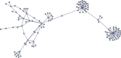
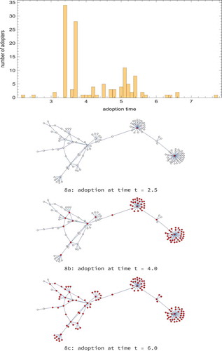
Figure 8. The top panel above shows the distribution of the peak adoption times of the nodes (companies) of the real network of Figure 7, the cooperation network of the Top 150 companies in South Tyrol, according to the Bass model in the first moment closure (Equation (13)), with parameters $q=0.35$, $p=0.03$. The adoptions in the two largest clusters are clearly visible at times 3.4 and 3.7 and those of their hubs at 2.2 and 2.4. The three panels 8a, 8b, 8c correspond to snapshots of the network at time $t=2.5$, $t=4.0$ and $t=6.0$. In each of them, the red ones in the online version (correspondent to the dark ones in the printed version) are the nodes which have adopted, whereas the white ones in the online version (light in the printed version) are the nodes which have not adopted.

Like for the Barabasi-Albert networks mentioned above, the equations system are obtained formally from a first moment closure, but in practice they give a better description of the real situation, because we can suppose that the continuous variable $X_i$, with $0\le X_i\le 1$, represents the adoption level of the innovation inside Company $i$; in other words, whereas in applications of the Bass model to the innovation adoption process of single individuals, $x_i$ jumps from 0 to 1 in a discontinuous way, here (for companies) $X_j$ evolves in a continuous way, like the average $0\le ⟨x_i⟩\le 1$ for individuals over many realizations.

The detailed solution of the Equations (13) for our real network (depicted in Figure 7) displays some interesting features.

(1) Looking at the adoption times of the nodes of degree 1 (compare histogram in Figure 8), one finds as expected that those belonging to the same cluster adopt in the same time, since they can be regarded as identical. For instance, in the cluster of the largest hub, their adoption time is $t_{max}=3.4$ (for the hub itself, $t_{max}=2.2$); in the cluster of the second-largest hub, the adoption time is $t_{max}=3.7$ (for the hub: $t_{max}=2.4$). What is the origin of the differences between clusters? Clearly, if the hub of a cluster is connected to the rest of the network better than the hub of another cluster, then it will adopt earlier and will consequently ‘infect’ earlier its cluster. In the SI epidemic model, which is equivalent to a Bass model with $p=0$ (pure contagion, no publicity/innovation term), this would actually be the only possible explanation of the difference between the two hubs. In the Bass model, however, the publicity term plays an essential role, because each degree-1 node in a cluster has an ‘individual’ adoption probability due to the $p$-term and independent of the state of its neighbours. After adoption, each degree-1 node tends to infect its hub, and the hub, in turn, re-destributes the influence on the whole cluster. In the end, therefore, the largest hubs tend to adopt earlier, like parents of large families where each kid keeps bringing home new ideas or gadgets.

(2) Since the network contains, as also evident from Figure 7, two large communities with different adoption times, if we plot the curves $f_{comm}(t)$ of the total adoption rates for each of these communities, their peaks are shifted. Therefore, the $f_{tot}(t)$ curve for the entire network will have a multi-modal character; even if this does not show up in separate peaks, the consequence is that the plot of $f_{tot}(t)$ is deformed in comparison to the standard logistic curve of the homogeneous Bass model (and also compared to the curve of the network Bass model in mean-field approximation). It is possible to check this deformation by trying, with no success, to fit $f_{tot}(t)$ with the usual Bass logistic function $f_{Bass}(t)=a^2{p}^{-1}{e}^{-at}[1+(q/p)e^{-at}{]}^{-2}$, where $a=p+q$. All this must be taken into account when the Bass diffusion is modelled through an agent-based simulation, like in [5], where the results are fitted with the Bass logistic function.

6. Conclusion

The dynamics of diffusion of innovations and information on social networks have attracted considerable attention in the last years. From the mathematical point of view, the most distinctive feature of a social network is its assortativity, defined in terms of the Newman coefficient $r$ and of the average nearest neighbour degree function $k_{nn}(k)$. In this work, we have developed new techniques for the construction of assortative correlation matrices and discussed some peculiar features of these matrices. We have then employed the correlation matrices for the numerical computation of the diffusion curves of the Bass model, which is widely used in marketing analysis. The Bass model offers the advantage, in comparison to other epidemic models, that the so-called diffusion peak time and takeoff time are well defined, independently of the initial conditions; they depend only on the empirical model parameters (innovation and imitation coefficient) and on the features of the network (scale-free exponent, assortativity). We have thus been able to study relations between these quantities that can be helpful in the analysis of real diffusion data.

Disclosure statement

No potential conflict of interest was reported by the authors.

Notes

1. Of course, the value of $\gamma$ in general changes if a different $n$ is taken.

2. We should point out here that, as explained in [7], when results relative to systems on scale-free networks with different exponents $\gamma$ are to be compared, the coefficient $q$ has to be normalized. And this is achieved by dividing $q$ by the average degree of the network $⟨k⟩=\sum _{k=1}^{n}kP(k)$.

3. Notice that several entries seem here to have the same value. In fact, this is simply due to rounding.

References

- F.M. Bass, A new product growth for model consumer durables, Management Sci 15 (1969), pp. 215–227. doi:10.1287/mnsc.15.5.215.
- V. Mahajan, E. Muller, and F.M. Bass, New product diffusion models in marketing: a review and directions for research, J. Marketing 54 (1990), pp. 1–26. doi:10.1177/002224299005400101.
- N. Meade and T. Islam, Modelling and forecasting the diffusion of innovation - a 25-year review, Int. J. Forecasting 22 (2006), pp. 519–545. doi:10.1016/j.ijforecast.2006.01.005.
- R. Guseo and M. Guidolin, Cellular automata and Riccati equation models for diffusion of innovations, Stat. Methods Appl. 17 (2008), pp. 291–308. doi:10.1007/s10260-007-0059-3.
- C.E. Laciana, S.L. Rovere, and G.P. Podestà, Exploring associations between micro-level models of innovation diffusion and emerging macro-level adoption patterns, Physica A 392 (2013), pp. 1873–1884. doi:10.1016/j.physa.2012.12.023.
- R. Pastor Satorras, C. Castellano, P. Van Mieghem, and A. Vespignani, Epidemic processes in complex networks, Rev. Mod. Phys. 87 (2015), pp. 925–979. doi:10.1103/RevModPhys.87.925.
- M.L. Bertotti, J. Brunner, and G. Modanese, The Bass diffusion model on networks with correlations and inhomogeneous advertising, Chaos Soliton Fract 90 (2016), pp. 55–63. doi:10.1016/j.chaos.2016.02.039.
- M.L. Bertotti, J. Brunner, and G. Modanese, Innovation diffusion equations on correlated scale-free networks, Phys. Lett. A 380 (2016), pp. 2475–2479. doi:10.1016/j.physleta.2016.06.003.
- M. Boguna and R. Pastor Satorras, Epidemic spreading in correlated complex networks, Phys. Rev. E 66 (2002), pp. 047104. doi:10.1103/PhysRevE.66.047104.
- M. Boguna, R. Pastor Satorras, and A. Vespignani, Absence of epidemic threshold in scale-free networks with degree correlations, Phys. Rev. Lett. 90 (2003), pp. 028701. doi:10.1103/PhysRevLett.90.094302.
- A. Barrat, M. Barthelemy, and A. Vespignani, Dynamical Processes on Complex Networks, Cambridge University Press, Cambridge, UK, 2008.
- M.E.J. Newman, The structure and function of complex networks, SIAM Review 45 (2003), pp. 167–256. doi:10.1137/S003614450342480.
- A.-L. Barabasi, Network Science, Cambridge University Press, Cambridge, UK, 2016.
- M.E.J. Newman, Assortative mixing in networks, Phys. Rev. Lett. 89 (2002), pp. 208701. doi:10.1103/PhysRevLett.89.208701.
- M.E.J. Newman and J. Park, Why social networks are different from other types of networks, Phys. Rev. E 68 (2003), pp. 036122. doi:10.1103/PhysRevE.68.036122.
- M.E.J. Newman, Mixing patterns in networks, Phys. Rev. E 67 (2003), pp. 026126. doi:10.1103/PhysRevE.67.026126.
- R. Xulvi-Brunet and I.M. Sokolov, Reshuffling scale-free networks: from random to assortative, Phys. Rev. E 70 (2004), pp. 066102. doi:10.1103/PhysRevE.70.066102.
- M. Catanzaro, G. Caldarelli, and L. Pietronero, Assortative model for social networks, Phys. Rev. E 70 (2004), pp. 037101. doi:10.1103/PhysRevE.70.037101.
- Z. Pan, X. Li, and X. Wang, Generalized local-world models for weighted networks, Phys. Rev. E 73 (2006), pp. 056109. doi:10.1103/PhysRevE.73.056109.
- C.C. Leung and H.F. Chau, Weighted assortative and disassortative network model, Physica A 378 (2007), pp. 591–602. doi:10.1016/j.physa.2006.12.022.
- M. Karsai, G. Iñiguez, K. Kaski, and J. Kertész, Complex contagion process in spreading of online innovation, J. Roy. Soc. Interface 11 (2014), pp. 20140694. doi:10.1098/rsif.2014.0694.
- T.M.A. Fink, M. Reeves, R. Palma, and R.S. Farr, Serendipity and strategy in rapid innovation, Nat. Commun. 8 (2017), pp. 2002. doi:10.1038/s41467-017-02042-w.
- G. Armano and M.A. Javarone, The beneficial role of mobility for the emergence of innovation, Sci Rep. 7 (2017), pp. 1781. doi:10.1038/s41598-017-01955-2.
- I. Iacopini, S. Milojević, and V. Latora, Network dynamics of innovation processes, Phys. Rev. Lett. 120 (2018), pp. 048301. doi:10.1103/PhysRevLett.120.048301.
- P. Lorenz-Spreen and B.M. Mnsted, Acceleraing dynamics of collective attention, Nat. Commun. 10 (2019), pp. 1759. doi:10.1038/s41467-019-09311-w.
- S. Lehmann and -Y.-Y. Ahn, Complex Spreading Phenomena in Social Systems, Springer, Cham, CH, 2018.
- M.L. Bertotti and G. Modanese, The Bass diffusion model on finite Barabasi-Albert networks, Complexity 2019 (2019), doi:10.1155/2019/6352657.
- J.P. Gleeson, S. Melnik, J.A. Ward, M.A. Porter, and P.J. Mucha, Accuracy of mean-field theory for dynamics on real-world networks, Phys. Rev. E 85 (2012), pp. 026106. doi:10.1103/PhysRevE.85.026106.
- M.E.J. Newman, Networks. An Introduction, Oxford University Press, Oxford UK, 2010.
- M.A. Porter and J.P. Gleeson, Dynamical Systems on Networks, Springer, Cham CH, 2016.