Carbon taxes and agriculture: the benefit of a multilateral agreement

ABSTRACT

Reducing greenhouse gas emissions from agriculture is crucial to reach global and regional climate targets. However, the efficiency of unilateral climate policies aimed at taxing emissions might be hampered by carbon leakage. One way to eliminate leakage is to implement a global carbon tax. In this article, we study the effects of a carbon tax in agriculture on GHG emissions by simulating five policy scenarios using the CAPRI model; (i) an EU tax, (ii) an EU tax complemented with a border carbon adjustment mechanism (BCA), (iii) a global tax, (iv) a global tax scaled by GDP per capita, and (v) a low global tax at 1/10 of the tax level in the other scenarios. For the global scenarios, we also analyse the impact on food consumption and nutrient intake. We find that a global tax of EUR 120 per ton CO₂-eq could reduce global agricultural emissions by 19%, but also jeopardizes food security in some parts of the world. A global tax at 1/10 of that rate (EUR 12) achieves a 3.2% reduction. In contrast, a unilateral EU tax of EUR 120 per ton CO₂-eq, accompanied with a BCA, reduces global agricultural emissions by only 0.15%.

Key policy insights

• A unilateral carbon tax in the EU causes significant emission leakage. This result depends strongly on differences in emission intensities between regions and on consumer preferences.

• A EUR 12 global carbon tax achieves a considerably larger global emission reduction than a EUR 120 unilateral EU carbon tax accompanied with a border carbon adjustment.

• A global carbon tax differentiated by GDP per capita is less effective than a uniform global carbon tax, as producers with higher emission intensities tend to get lower tax rates. Other ways of taking equity into account should be sought when designing climate policies in the agricultural sector.

KEYWORDS:

• Climate change mitigation
• agricultural emissions
• economic assessment
• economic model
• carbon leakage
• food security

1. Introduction

The agricultural sector emits about 16% of all anthropogenic greenhouse gases (GHGs) driving global warming, excluding energy use in agriculture and emissions caused by land use and land use change (Ritchie & Roser, 2020). So far, efforts to mitigate GHG emissions from agriculture have been scant and insufficient (OECD, 2019). Policymakers increasingly recognize environmental policies targeting agriculture as paramount in climate change mitigation (IPCC, 2022). For example, in a recent communication, the European Commission presents a vision of how to make Europe climate-neutral in 2050, emphasizing the importance of reducing GHG emissions from agriculture (European Commission, 2018). A potentially efficient policy approach is to price GHG emissions in accordance with the polluter pays principle. A carbon tax, for example, sets a price on GHG emissions (Baranzini et al., 2017). By letting emitters pay for the damage they cause, the market failure behind global warming is addressed (Nordhaus, 2019). Agriculture has largely been exempted from such pricing instruments and emission trading (OECD, 2019).

A risk, not yet fully addressed for agriculture, is that a carbon tax may be undermined by carbon leakage (Arvanitopoulos et al., 2021). Introducing a carbon tax in a single country, or a small region like the EU, may reduce GHG emissions in the region, but will also weaken the international competitiveness of that region, triggering an increase in production and emissions in countries not adopting the tax (Copeland & Taylor, 2005; Elliott et al., 2010). Increased GHG emissions elsewhere can offset the emission reductions, partly or completely. A growing literature uses agricultural simulation models to assess the impacts of carbon taxes on production, international trade, commodity prices, GHG emissions and carbon leakage (Dumortier et al., 2012; Dumortier & Elobeid, 2021; Zeck & Schneider, 2019). Various trade-related measures to limit carbon leakage have been analysed, like border carbon adjustments and environmental standards for imported goods (Böhringer et al., 2014; Fischer & Fox, 2012; Nordin et al., 2019). The studies show that such measures may lessen the leakage to some extent, although they are unlikely to be effective in export-oriented sectors. It is further argued that carbon pricing needs complementing policies to reduce carbon leakage, for example, policies that encourage using GHG abatement practices (Henderson & Verma, 2021) or consumption taxes (Böhringer et al., 2017).

Another way to reduce carbon leakage is to increase the number of countries adopting the tax (Antimiani et al., 2013; Henderson & Verma, 2021), and with a global tax, there would be no leakage (Baranzini et al., 2017). However, such a tax opens questions of fairness and food security in developing countries, where GHG emissions can be high and agricultural exports often are important for foreign exchange earnings (Arvanitopoulos et al., 2021; Frank et al., 2017; Jensen et al., 2019). Moreover, efficiency differences between countries, as captured by differences in emissions per produced kg of agricultural commodities (emission intensities, EIs), suggest that energy efficiency improvements can be made for high emitters (Schneider & Smith, 2009). This is an argument for including developing countries in a global carbon tax agreement, thereby introducing incentives to harness this potential.

The aim of this paper is to quantify the potential emission reductions of a global carbon tax versus an ambitious unilateral carbon tax in the EU, thereby contributing to the literature on climate policy in agriculture. To this end, we compare the impact of an EU tax against an EU tax with a BCA and three versions of a global tax; a high uniform tax, a low uniform tax and a tax differentiated according to GDP/capita. We also investigate how different versions of the global tax would affect global food consumption. The quantitative analysis uses the agricultural partial simulation model CAPRI. This study also updates, documents and publishes the CAPRI model estimates of GHG EIs for global regions outside the EU, useful for computing impacts on carbon leakage in agriculture.

2. Methodology

We use a global, partial, comparative static equilibrium model of agricultural production and trade (CAPRI) to study the impacts of carbon taxes and BCA. We calibrate the model to a baseline without carbon taxes for the year 2030, and study how equilibrium is disrupted by various taxes.

2.1. The CAPRI model

The CAPRI model is a global partial equilibrium model of agricultural markets and primary food processing. The primary GHG emissions from agriculture (methane and nitrous oxide) are linked to agricultural production in a detailed, endogenous GHG emission accounting system. The model has been developed and used in many applied studies since 1999 and has frequently been used to study the interactions between agriculture, international trade and greenhouse gas emissions (e.g. Barreiro-Hurle et al., 2021; Frank et al., 2019; Gómez-Barbero et al., 2020; Gren et al., 2021; Himics et al., 2018; Jansson et al., 2021). CAPRI contains two models that are interlinked. One is a global market model of supply, demand, primary processing and trade in agricultural commodities. The other is a set of agricultural supply models based on mathematical programming that is implemented for a subset of the countries of the world, with a higher degree of technological and geographical detail. In the present study, the focus is on international trade. Hence, most of our results come from the market model, which is presented below, while the supply models are outlined in Appendix 1.

The market model computes the equilibrium prices of 65 traded products, including primary agricultural outputs, young animals, processed products, and some aquatic products. All countries in the world are represented in the market model, either as individual countries or as part of a regional aggregate. In total, there are 79 market regions with their own consumption, production and processing sectors, see Appendix 2. Consumption is derived by applying Roy’s identity to an expenditure function with a flexible functional form (Generalized Leontief, see Ryan & Wales, 1999). Demand system parameters are specified to replicate given prices and quantities while maintaining regularity and minimizing the sum of squared deviations from the elasticity matrices given by Muhammad et al. (2011). By including a ‘rest’ good, the system accounts for varying shares of expenditure spent on food. Production of traded commodities is modelled with supply functions derived from a normalized quadratic profit function so that the supply of each output and intermediate input depends on the prices of all other outputs and inputs. The 79 regions form 44 trade blocs. The model computes trade flows between all pairs of trade blocs based on a two-stage Armington (1969)¹ specification working with Constant Elasticity of Substitution (CES) functions and provides mechanisms for simulating trade instruments such as tariffs and trade quotas. This implies that domestic and imported goods are treated as imperfect substitutes, a widely used assumption in applied trade models. Between regions or countries within the same trade bloc, in contrast, only net trade is simulated. Dairies, bulk feed production and vegetable oil production are included and modelled with normalized quadratic profit functions and equations for the preservation of milk fat and protein. The consumer price is related to the commodity price by a fixed, additive markup, specific to each regional market, representing all costs incurred in the supply chain except for international trading costs, which are separately modelled.

CAPRI is comparative static. That means that it starts with an economic equilibrium and computes how changes to restrictions, policies or other model parameters disrupt that equilibrium. The initial equilibrium is assumed to represent a point of time in the future, in our case 2030, and it is created by a calibration of the model to a so called ‘baseline’. The baseline is created based on historical data series and econometric forecasts in the annual Agricultural Outlook of the European Commission. The calibration means that selected parameters of the model, governing how agents such as consumers and producers behave, are adjusted so that the baseline is in equilibrium, i.e. the prices are such that the agents choose to produce and demand precisely the amounts found in the baseline. The baseline coincides with the reference scenario in our analysis.

2.2. Scenarios

We compute the following scenarios:

• REF: The reference scenario implies a full implementation and then continuation of the current common agricultural policy (CAP 2014–2020) until 2030.

• EUTAX: As REF, plus an emission tax of 120 EUR/ton carbon dioxide equivalent (CO₂-eq) levied on agricultural production in all EU countries.

• EUTAXBCA: As EUTAX plus a border carbon adjustment (BCA) for imports to the EU. The tariff level for imported commodities is the same as the producer tax in the EU, 120 EUR/ton CO₂-eq.

• GLOBTAX: As REF plus a global emission tax of 120 EUR/ton CO₂-eq levied on agricultural outputs.

• GLOBTAXPROP: As GLOBTAX, but the tax level is scaled by GDP per capita in each region in relation to the average in Western Europe. Since Western Europe is an affluent region, this scenario reduces the global average tax level.

• GLOBTAXLOW: As GLOBTAX, but at a tenth of the tax rate (12 EUR/ton CO₂-eq).

Our analysis only considers non-CO₂ emissions related to the UNFCCC category ‘agriculture’ (methane (CH₄) and nitrous oxide (N₂O)), i.e. excludes CO₂ emissions, land use, land use change and forestry (LULUCF), and other emissions upstream or downstream from agriculture. The tax and the tariff are based on the Swedish carbon dioxide emission tax on fossil fuels (1150 SEK/ton). In the simulations, the tax is inflated by 1.9% per year from 2018 to 2030, resulting in about 150 euro/ton in nominal terms. The tax is a producer tax, implemented as a fixed amount per kg of product at the farm gate, computed by multiplying each commodity’s EI by the tax rate. The EIs are based on average emissions for the commodities in each region at the regional farm gate, arising in agricultural processes in that region and assigning them to products that (potentially) are sold from the regional farm. The farm gate concept assigns emissions from intermediate inputs (e.g. grazing) to the final output (e.g. meat), whereas emissions from the production of tradable inputs produced by agriculture, notably feeding concentrates, are assigned to the feedstock crop where it was produced² and not to the final good. The tax per ton of product is defined before the simulation and kept constant in simulation. This way of modelling the tax implies that the producers cannot avoid the tax by implementing GHG mitigation technologies that lower EI, but only by changing their production mix towards products with a smaller carbon footprint. This implementation, on the one hand, makes the tax less efficient than it would be if linked to the production technology. On the other hand, it is simple enough to implement even in countries with less developed administrative control structures.³ The tax can represent other costly mitigation measures that shift agricultural supply functions upwards, reducing the production of polluting commodities.

In EUTAX, the EU introduces a unilateral tax. This is expected to induce emission leakage, and hence, accompanying the tax with a BCA could be justified. In EUTAXBCA, importers pay a climate tariff at the EU border. For computing the BCA, we modified the EI in the country of origin of animal products that are imported to the EU to take into account the emissions caused in the production of tradable feeding stuffs used in the agricultural production process abroad.⁴

GLOBTAX represents an ambitious global carbon tax agreement. A tax affecting poorer regions to a lesser extent could be a more realistic approach. This motivates GLOBTAXPROP. Another possibility is a uniform but low carbon tax for agriculture, represented by GLOBTAXLOW.

2.3. Data and estimation of GHG emission intensities

The estimations of GHG EIs and the associated accounting framework of CAPRI have been developed in several studies by several researchers, e.g. Domínguez et al. (2016), and further extended with new data and revised methods for this study. We, therefore, see fit to provide an overview of the present methods in the supplementary material (Appendix 3), as well the results of the estimations (electronic supplement). Underlying data and methods for the estimations are from OECD (2015), IPCC (2006) and FAO (2018). Figure 1 summarizes results for key commodities and regions.

Figure 1. Emission intensity estimates for selected commodities and regions of the world in 2030. Left panel: for animal products. Right panel: for crop products.

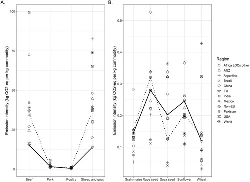
Beef is most important, as it is widely traded and its production causes high emissions. In our estimates, the global average (formed using the production quantities of the baseline) is 35 kg CO₂-eq/kg. The EU and USA have low emissions associated with beef production by international standards, in particular, compared with India and the least developed countries (LDCs) in Africa (Africa LDCs other). This is in line with the EIs reported by FAO (2022). Their (our) estimates of CO₂-eq/kg for beef in the EU, USA and India are 15 (15), 12 (16) and 108 (99), respectively. Sheep and goat meat has similarly high EIs as beef, whereas pork and poultry EIs are significantly lower. These EIs also align with FAO (2022).

Among animal feed products, soy is of particular interest since it is produced in large quantities and widely used as animal feed. The estimates for Brazil and Argentina stand out, with low values for both countries. This result is due to low application rates of synthetic fertilizers in the underlying data, leading to low emissions of N₂O associated with fertilizer turnover, in combination with low reported GHG emissions of N₂O from crop residues.

The production-side emission accounting becomes cumbersome when we combine an emission tax in production with a BCA. The EIs used for computing the production tax do not include emissions embodied in animal feed purchased at the market since those inputs are already taxed upon production. For the BCA, however, we want to tax all agricultural emissions embodied in the product at the border, i.e. including animal feed used overseas. To this end, we use a set of EIs that has been modified to take feed use into account. The computation of these modified EIs is similar to the estimation of the production-side coefficients discussed above.

The EIs of some products vary a lot between countries. This is mostly explained by the official IPCC methods used for computing them: e.g. a more or less fixed emission per animal is divided by a highly variable yield per animal. That is, in regions where many animals live longer but yield less meat, the EIs can be rather high per kg output. For some estimates, however, the differences between countries seem unreasonably large, perhaps due to data deficiencies. We address this issue in the sensitivity analysis.

2.4. Sensitivity analysis

The estimated EIs have a strong influence on the results of studies such as this. Therefore, the robustness of the estimates is of interest, and further work on deriving statistics such as standard deviations is needed. The variation in some estimated EIs is large, e.g. methane from enteric fermentation ranging from 259 to 3795 kg per ton beef, raising the issue of outliers. We, therefore, repeated all the simulation experiments with an alternative set of estimates, where we have shrunk the EIs towards the global average. The shrinkage can be motivated from a statistical point of view as shrinkage is known to be capable of reducing the mean squared error of predictions, at the cost of introducing a bias in the estimation (e.g. Robbins, 1964). The ratio of regional EI $\left(\mathrm{E}{\mathrm{I}}_r\right)$ to world average EI $\left(\mathrm{E}{\mathrm{I}}_{\mathrm{glob}}\right)$ was reduced by the square root, thus affecting EI estimates far from the global average more than estimates closer to the global average. Formally, we computed a factor $z_r$ for each region r that determines the shrunk ${\mathrm{EI}}_r^{\ast }$ as a function ${\mathrm{EI}}_r^{\ast }=\mathrm{E}{\mathrm{I}}_r{z}_r$ by requiring that the ratio of regional to global EI shrink as the exponential function ${\displaystyle \frac{{\mathrm{EI}}_r^{\ast }}{\mathrm{E}{\mathrm{I}}_{\mathrm{glob}}}={\left({\displaystyle \frac{\mathrm{E}{\mathrm{I}}_r}{\mathrm{E}{\mathrm{I}}_{\mathrm{glob}}}}\right)}^{1/2}}$. The factor $z_r$ was computed for REF and applied in the computation of tax rates and emission results in the sensitivity experiment relating to EIs. Changing the EIs this way reduces the global volume of emissions in REF. Therefore, an additional reference scenario was computed, and in the results section, we present the impact compared to the relevant reference scenario for the sensitivity experiment (Shrink in Figures 2 and 3).

Figure 2. Mitigation in the EU and leakage to non-EU countries in the unilateral scenarios. Million tons CO₂-eq annually, difference to reference scenario. Lines at the end of the bars indicate the range of outcomes in the sensitivity analyses.

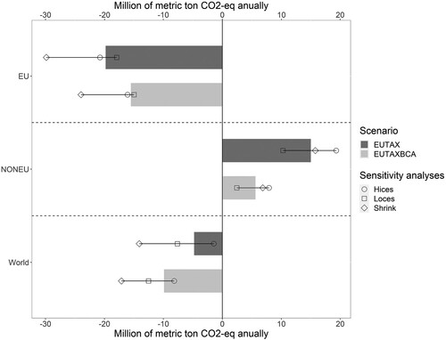
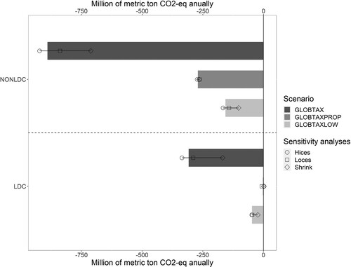
Figure 3. Mitigation in LDC and non-LDCs in the global scenarios. Million tons CO₂-eq annually, difference to REF. Lines at the end of the bars indicate the range of outcomes in the sensitivity analyses.

Another important parameter is the substitution elasticity in consumption. In CAPRI, consumers treat domestic and imported goods as imperfect substitutes, and the substitution elasticity steers the extent to which domestic products are replaced with imported substitutes when prices change. This affects the rate of emissions leakage. In REF, they are set to values that vary by commodity from 2 up to 6 with lower values for animal products and higher for crop products based on elasticities from the literature reported by Ahmad et al. (2020, p. 16) and established CAPRI parameters. Appendix 4 lists all the substitution elasticity values used in this study. The substitution elasticities are important for the results, yet uncertain. Bajzik et al. (2020) carry out a meta-analysis that is not product specific and suggest using values from 2.5 to 5.1, broadly supporting the values we use. In our sensitivity analyses, we ran additional simulations where all CES parameters were 50% higher or lower than in the standard setting (Hices and Loces in Figures 2 and 3).

3. Results

3.1. Taxes and price changes

The taxes cause producer prices to decrease and consumer prices to increase. When demand is less elastic than supply, consumer prices tend to increase more than producer prices decrease. Table 1 shows taxes, producer prices and consumer prices in selected regions (EU, LDCs and World) for beef and wheat in all scenarios. We focus on beef markets, where taxes and price impacts are larger and more diverse than wheat. In EUTAX and EUTAXBCA, it is difficult for EU producers to transfer the tax burden to the consumers, and EU beef producer prices drop by 920 euro (20%) and 612 euro (13%), respectively, whereas consumer prices of the aggregate of domestic and imported beef increase by 1340 euro (15%) and 1708 euro (19%) respectively.

Table 1. Taxes, producer prices (Pp) and consumer prices (Pc) in all scenarios for selected products and regional aggregates.

Product	Region	Item	REF	EUTAX	EUTAXBCA	GLOBTAX	GLOBTAXLOW	GLOBTAXPROP
Beef	EU	Tax	0	2304	2304	2307	236	2191
Beef	EU	Pp	4603	3683 (−20%)	3991 (−13.3%)	4727 (2.7%)	4599 (−0.1%)	4016 (−12.7%)
Beef	EU	Pc	9139	10,479 (14.7%)	10,847 (18.7%)	11,561 (26.5%)	9369 (2.5%)	10,716 (17.3%)
Beef	LDC	Tax	0	0	0	12,287	1192	267
Beef	LDC	Pp	3818	3844 (0.7%)	3837 (0.5%)	1482 (−61.2%)	3436 (−10%)	3859 (1.1%)
Beef	LDC	Pc	4399	4431 (0.7%)	4425 (0.6%)	13,585 (208.8%)	5212 (18.5%)	4787 (8.8%)
Beef	World	Tax	0	181	184	4562	516	1889
Beef	World	Pp	3787	3741 (−1.2%)	3761 (−0.7%)	3444 (−9.1%)	3698 (−2.4%)	3521 (−7%)
Beef	World	Pc	6814	6949 (2%)	6970 (2.3%)	11,398 (67.3%)	7284 (6.9%)	8401 (23.3%)
Wheat	EU	Tax	0	18	18	18	2	14
Wheat	EU	Pp	173	163 (−5.6%)	166 (−4%)	168 (−2.6%)	172 (−0.3%)	167 (−3.3%)
Wheat	EU	Pc	2723	2730 (0.2%)	2735 (0.4%)	2736 (0.5%)	2724 (0%)	2731 (0.3%)
Wheat	LDC	Tax	0	0	0	21	2	1
Wheat	LDC	Pp	233	236 (1.2%)	236 (1.4%)	223 (−4.3%)	232 (−0.5%)	236 (1.3%)
Wheat	LDC	Pc	534	537 (0.6%)	538 (0.8%)	548 (2.6%)	535 (0.3%)	540 (1.1%)
Wheat	World	Tax	0	3	3	20	2	7
Wheat	World	Pp	201	201 (0%)	202 (0.2%)	198 (−1.5%)	201 (−0.2%)	200 (−0.7%)
Wheat	World	Pc	1555	1558 (0.2%)	1559 (0.3%)	1572 (1.1%)	1557 (0.1%)	1561 (0.4%)

In GLOBTAX, EU consumer prices of beef increase more than in the unilateral scenarios (+2422 euro), but the increase is much larger in regions with high-emission factors such as LDCs (+9186 euro, or 209%). Producer prices in regions with high EIs decrease dramatically (−61% in LDCs). EU producer prices, in contrast, increase (+3%) when global demand shifts towards the less taxed EU beef. Conversely, in GLOBTAXPROP, producer prices in LDCs increase by 1% by the same mechanism.

3.2. GHG emissions and leakage

3.2.1. Unilateral agreements

EUTAX induces a reduction in regional agricultural emissions in the EU of 20 million metric ton CO₂-eq annually (5.5% of EU agricultural emissions, top dark grey bar in Figure 2). However, global emissions decrease by only 4.8 million metric ton CO₂-eq (0.074% of global agricultural emissions, bottom dark grey bar in Figure 2). Hence, most of the mitigation in the EU (76%) is offset by increased emissions outside the EU (NONEU in Figure 2).

In EUTAXBCA, regional agricultural emissions in the EU decrease by 16 million metric ton CO₂-eq (4.3% of EU agricultural emissions, top light grey bar in Figure 2), while global emissions decrease by 9.9 million metric ton CO₂-eq (0.15% of global agricultural emissions, bottom light grey bar in Figure 2). This means that 36% of the emissions mitigation in the EU is offset by increased emissions outside the EU. Hence, with a BCA, the mitigation impact of a unilateral carbon tax is much stronger. When imports must pay for embedded GHG emissions, EU consumer prices can rise more relative to foreign markets (Table 1). EU consumers thus bear a larger share of the tax and less EU production is replaced by imports.

In EUTAX, changes in regional emissions are driven by a few animal products: beef, pork, sheep and goat meat (SGMT) and milk. Beef production accounts for the largest share of the reduced emissions in the EU, 47% (9.2 million tons). However, on a global scale, the decrease in emissions from beef production is only 0.99 million tons. This can largely be attributed to considerable differences in EIs for EU and non-EU production since only 36% of the reduced production in EU is replaced by non-EU production. Cereal production is also a large contributor to reduced emissions in the EU in EUTAX, due to the large quantities produced, 18% of the total reduction (3.6 million tons). Of the reduced EU production 20% is replaced by non-EU production. However, non-EU production is slightly less emission-intensive, and cereal production, therefore, contributes to the largest share of the reduced emissions globally, 64% (3.0 million tons).

In EUTAXBCA, the changes in emissions largely follow the same pattern as in EUTAX. Generally, the BCA prevents that reduced EU production is replaced by imports, and hence, emission leakage is smaller than in EUTAX. This is apparent concerning beef production, where only 20% of the reduced EU production is replaced by non-EU production. Emissions from beef production in the EU are reduced by 7.8 million tons in EUTAXBCA. However, due to the larger EIs in non-EU production, the global emissions from beef production only shrink by 2.9 million tons. The BCA is particularly effective in the SGMT and dairy markets, where global emissions decrease more than EU emissions. This is because the BCA reduces EU demand for imports, and if non-EU producers cannot easily replace exports to the EU with increased exports to other markets, they reduce production and emissions. This effect causes global emissions from SGMT production to decrease by 2.7 million tons, while EU emissions from SGMT production decrease by just 0.052 million tons.

3.2.2. Multilateral agreements

In GLOBTAX, global agricultural emissions decrease by 1200 million metric ton CO₂-eq (19% of global agricultural emissions), i.e. 120 times as much as in EUTAXBCA (dark grey bars in Figure 3). This indicates that a carbon tax is much more efficient in other regions than the EU, as the EU share of world agricultural production is 11%.⁵ With an equally efficient carbon tax across regions, the reduction would have been in proportion to the EU share of production. Carbon leakage arises as a consequence of differences in environmental policy. Since the tax is uniform on a global level, by definition, no emission leakage occurs. A large share (26%) of the emission reduction takes place in LDCs despite their much smaller share (5.5%) in total agricultural production⁵ because their EIs in are generally higher than those of non-LDCs.

In GLOBTAXPROP, global emissions decrease by 270 million metric ton CO₂-eq (4.2% of global agricultural emissions, medium grey bars in Figure 3). That is less than in GLOBTAX, for two reasons: Many countries have much lower income per capita than Western Europe, and hence the global average tax level is lower in this scenario. The global average tax on beef becomes 1889 euro per metric ton of product compared to 4562 euro in GLOBTAX. Furthermore, many poorer countries have higher EIs, and the tax therefore tends to become lower where emissions are higher and vice versa. In the LDCs, there is almost no abatement at all since the low tax there is entirely offset by higher world market prices that result from a lower global supply.

In GLOBTAXLOW, global emissions decrease by 200 million metric ton CO₂-eq (3.2%, light grey bars in Figure 3). While the tax rate in GLOBTAXLOW is only 10% of the rate in GLOBTAX, the emission reduction is 17%. This indicates that the marginal abatement effect of a global uniform emission tax decreases with increasing tax rates.

3.2.3. Food security – calorie consumption

In this section, we only include the scenarios with global taxes. The reason is that EU is a relatively affluent region, which only accounts for about 13% of the globally produced calories in REF, and the scenarios with unilateral measures in the EU, therefore, have a limited impact on global food security. We computed the consumption of energy in all model regions by multiplying consumed food quantities with standard nutrient content factors.

In GLOBTAX, global calorie consumption decreases by 0.50%. Among individual commodities, the consumption of sheep and goat meat (−24%) and beef meat (−17%) decrease most strongly. The reduction in calorie intake caused by the lower consumption of those commodities is offset by the increased consumption of products subject to lower taxes, such as pork, poultry, cereals, and vegetables.

Looking at the regional impacts, one might expect a more severe impact on calorie consumption in poorer countries due to the negative correlation between prosperity and EI in ruminant production. However, the results don’t allow any such general conclusions. Even though the largest negative impacts on energy intake are found among the poorer countries, e.g. in Ethiopia (−8.42%) and Vietnam (−3.19%), there are also many poor countries in which energy intake increases, e.g. Bolivia (+1.61%) and Paraguay (+2.03%). In those cases, the shift away from ruminant meat to other products is sufficiently large to compensate for the loss in energy intake. This is possible because consumers (in the model) do not deliberately demand ‘energy’ but try to satisfy their preferences for different products based on prices and their available budget and because the diet is dominated by crop products rather than ruminant meat. Reducing meat consumption by say 10% and instead increasing cereals consumption by 10%, from a point where cereals consumption already is much higher than meat consumption in absolute terms, can result in an increase in energy intake and be economically feasible, albeit less attractive to the consumer than the pre-tax situation.

In GLOBTAXPROP, i.e. where the tax level is scaled by GDP per capita in each region in relation to the average in Western Europe, global calorie consumption decreases by 0.079%. Thus, the effect on global consumption is smaller than in GLOBTAX. The composition of consumption changes, away from beef and SGMT towards more pork, poultry, cereal, and vegetable consumption. The impact on the poorest countries of the world is smaller than in GLOBTAX, whereas the impact on richer countries is larger. The country that experiences the largest decrease is Norway (−0.61%). Other wealthy countries are also among the most affected, e.g. Japan (−0.56%) and Switzerland (−0.53%). None of the poorer nations severely affected by GLOBTAX experiences a similar effect on calorie consumption in GLOBTAXPROP. This can be attributed to the fact that GLOBTAXPROP does not induce a change in consumed commodities to the same extent as GLOBTAX.

In GLOBTAXLOW, global calorie consumption only decreases by 0.069%. The regional impacts are similarly distributed as in GLOBTAX, but smaller. Ethiopia and Vietnam are most severely affected, with decreases of 1.0% and 0.37%, respectively.

4. Discussion

The purpose of this study was to quantify the potential gains of a global carbon tax in agriculture versus an ambitious unilateral carbon tax in the EU (120 euro/ton CO₂). Our results indicate that a unilateral EU tax (EUTAX) is associated with considerable carbon leakage: 76% of the emission reduction within the EU is offset by increased emissions outside the EU. The high carbon leakage diminishes the global reduction in agricultural emissions, which in EUTAX is just 0.074%. When the EU tax is combined with a BCA on imports, the rate of leakage is reduced to 36%, and the global reduction in agricultural emissions is doubled to 0.15%. To alleviate carbon leakage, the carbon tax could be extended to include more countries.

If the ambitious EU carbon tax is applied to the whole world (GLOBTAX), the global agricultural GHG emissions are reduced by 19%, or about 1.2 Gt CO₂-eq per year, significantly contributing to a sustainable food system in terms of climate impact. Such a high tax rate has, however, dramatic impacts on, e.g. beef meat production in some regions where the EIs are high. Furthermore, consumer prices rise significantly, reducing the intake of energy in some poorer countries where food security is already a problem. Differentiating the global tax with respect to GDP per capita (GLOBTAXPROP) eases the food security problems but reduces the efficiency of the carbon tax; global emissions decline by only 270 Mt CO₂-eq (4.2%). Poorer regions tend to have less productive agriculture and, therefore, higher EIs per unit of output, whereas the opposite tends to hold true for the wealthier parts of the world. The differentiated tax thus tends to become higher where emissions are low and lower where they are high. If the global tax rate is reduced to 12 EUR/CO₂-eq for all countries (GLOBTAXLOW), the results show a global reduction of emissions of 200 Mt annually (3.2%), and less dramatic changes in production and consumption patterns in poorer regions of the world. Further, the reduction in global emissions per euro of tax rate is larger compared to a global tax 120 EUR/CO₂-eq (GLOBTAX), indicating that the marginal effect of the global tax is higher at the lower tax level but declines when the tax rate is higher.

The leakage rate that we find in the agricultural sector in the unilateral tax scenarios is larger than the leakage of CO₂ emissions found in fossil fuel-related sectors. Böhringer et al. (2012), summarizing the results of 12 different models, find an average leakage rate of 24% in the simulation of unilateral abatement by EU + EFTA (sensitivity run). Our high leakage is primarily driven by ruminant meat products, which have very different EIs in different countries (Figure 1). EU ruminant meat products have low EIs compared to the rest of the world; that is, the EU is highly productive in terms of GHG emissions per kg of ruminant product. A unilateral carbon tax on such a system inevitably results in large carbon leakage. We do not know enough about the parameters of the various models used in Böhringer et al. (2012) to explain why our leakage rates are larger.

Frank et al. (2019) also apply the CAPRI model to study the impacts of global carbon taxes and find about twice as high mitigation impacts as our results at a similar carbon tax level. The main explanation for the difference is that they tax emissions directly instead of applying the tax per commodity and allow for technological changes in the production of each product, so that the farms can reduce emissions in response to the tax by adopting specific mitigation technologies. Examples of such technologies are anaerobic manure processing, precision farming and fertilization, targeted breeding efforts, and the impact of endogenous feed mix changes. Henderson and Verma (2021) also include the use of GHG abatement policies among farmers facing the carbon tax, resulting in a lower carbon leakage than we find. We opted for the simpler implementation because sales of products is something that is already subject to measurements and taxation, making an actual implementation relatively simple in administrative terms, whereas the step to a global farm-level emission accounting system seems challenging at this point. The difference in outcome between our results and theirs broadly indicate the potential efficiency gains in mitigation that can be reached if the abatement measures can be set up to provide producers with incentives for technical change.

Our sensitivity analyses show that consumer behaviour strongly impacts on the carbon leakage that follows from unilateral climate policies. This holds for the real world as well as for the simulation model. If the substitution elasticities are higher than in the standard results (EUTAX), the leakage can approach 100%, but it might also be closer to 50% if CES elasticities are lower (circles and squares in Figure 2). Moreover, if the EIs are more homogeneous across the world than in our estimates, as in the Shrink sensitivity analysis, leakage is smaller and the global mitigation effect of unilateral measures in the EU higher (diamonds in Figure 2).

The CES parameters play less of a role with a global tax. However, the spread of the EIs (sensitivity analysis Shrink) directly impacts on the level of taxation and mitigation in LDC (Figure 3, lower panel). Less spread of the EIs means that less mitigation takes place in LDCs, with lesser implications on food security.

Even in GLOBTAX, global levels of calorie consumption remain stable. A key explanation is that producing high-emission animal products requires more land and other inputs than producing plant-based human food such as vegetables, cereals and pulses (Erb et al., 2016). A small reduction in animal production releases much land for crop production. Therefore, carbon tax impacts on food security can be further mitigated if human diets, for some reason, change more strongly from meat consumption towards plant-based foods, which could be produced on some of the land that is freed-up when meat production is reduced while also releasing land for other uses. Frank et al. (2019) study the impacts of dietary preference shifts and find that it could lead to large additional greenhouse gas mitigations when combined with low or moderate carbon tax levels, whereas the additional benefit of dietary shifts is smaller at high carbon prices.

5. Conclusions

To conclude, our analysis shows that a coordinated carbon tax policy is more effective than unilateral action. Even a modest global carbon tax would bring considerable mitigation, plucking the lowest-hanging fruit. A tax rebate for the poorer countries, as modelled here with a tax rate proportional to GDP per capita, does not appear to be a good way forward because the mitigation effect becomes much lower.

From the EU perspective, as for all countries that have relatively low EIs, the global tax can boost competitiveness. A carbon tax designed this way internalizes the public costs for emissions from the agricultural sector, creating a comparative advantage for countries that are more efficient in terms of emissions per ton product. The global tax would reduce global supply and raise consumer prices of many products. In regions with low tax rates, the negative impact of the tax on producer prices is smaller than the positive impact of the higher consumer prices. These regions will expand their production despite the shrinking global market. In countries where emissions per ton are higher, the converse happens.

A global carbon tax might meet resistance from countries that are bound to lose international competitiveness. Indeed, it may lead to negative social consequences if large numbers of farmers are driven out of business. Our results show that even a high global tax would decrease global calorie consumption by just 0.5%, even though the carbon tax does not provoke a global food security problem, the local impacts can be large when production shifts between countries, and at the level of household types, the impacts are likely to be larger still. Therefore, food security is not as much technical as an economic problem – there is enough food available globally, but some households cannot afford it.

How can the poorest households and farmers of the world be able to afford nutritious food under a global tax? This highlights the need to use tax revenues wisely. International re-distribution should be part of a global agreement (c.f. Baranzini et al., 2017; Fujimori et al., 2019). Tax revenues could be re-funded to compensate farmers in poorer countries, to support investments that make production more efficient in terms of GHG emissions, or to support restructuring of production to direct resources into less polluting sectors. The large variation in EIs across regions suggests that potential for efficiency gains exists, i.e. it seems possible for countries with high-emission intensities to catch up by adopting production technologies from countries with low emission intensities.

Notes

1 Differentiating first domestic from imported goods, then among imported goods from different origins.

2 This avoids double counting when imposing a tax at the farm gate. Traded inputs are treated somewhat differently in EUTAXBCA to avoid double counting.

3 For more flexibility, one could envisage the EI being updated on an annual basis, or some certification system recognizing several emission classes similar to the energy declaration of the EU.

4 This implies that if a foreign producer uses bulk feed from the EU to produce meat that is in turn exported to the EU, that bulk feed is double taxed by the BCA, which we consider a minor problem. Furthermore, we only computed additional taxes, ignoring the issue, likely to arise in practice, of how to discount for pre-existing environmental taxes and the use of inputs that are already taxed in the country of origin.

5 Metric tons primary production in the CAPRI database.

References

- Ahmad, S., Montgomery, C., & Schreiber, S. (2020). A comparison of Armington elasticity estimates in the trade literature (Economics Working Paper Series, 2020-04-A.GTAP Resources).
- Antimiani, A., Costantini, V., Martini, C., Salvatici, L., & Tommasino, M. C. (2013). Assessing alternative solutions to carbon leakage. Energy Economics, 36, 299–311. https://doi.org/10.1016/j.eneco.2012.08.042
- Armington, P. (1969). A theory of demand for products distinguished by place of origin. IMF Staff Papers, 16(1), 159–117. https://doi.org/10.2307/3866403
- Arvanitopoulos, T., Garsous, G., & Agnolucci, P. (2021). Carbon leakage and agriculture: A literature review on emissions mitigation policies (OECD Food, Agriculture and Fisheries Paper no 109). OECD. https://doi.org/10.1787/18156797.
- Bajzik, J., Havranek, T., Irsova, Z., & Schwarz, J. (2020). Estimating the Armington elasticity: The importance of study design and publication bias. Journal of International Economics, 127, 103383. https://doi.org/10.1016/j.jinteco.2020.103383
- Baranzini, A., van den Bergh, J. C. J. M., Carattini, S., Howarth, R. B., Padilla, E., & Roca, J. (2017). Carbon pricing in climate policy: Seven reasons, complementary instruments, and political economy considerations. WIREs Climate Change, 8(4), e462. https://doi.org/10.1002/wcc.462
- Barreiro-Hurle, J., Bogonos, M., Himics, M., Hristov, J., Perez Dominguez, I., Sahoo, A., Salputra, G., Weiss, F., Baldoni, E., & Elleby, C. (2021). Modelling environmental and climate ambition in the agricultural sector with the CAPRI model (Technical report by the Joint Research Centre (JRC), the European Commission’s science and knowledge service, JRC121368). https://EconPapers.repec.org/RePEc:ipt:iptwpa:jrc121368
- Böhringer, C., Balistreri, E. J., & Rutherford, T. F. (2012). The role of border carbon adjustment in unilateral climate policy: Overview of an energy modeling forum study (EMF 29). Energy Economics, 34, S97–S110. https://doi.org/10.1016/j.eneco.2012.10.003
- Böhringer, C., Fischer, C., & Rosendahl, K. E. (2014). Cost-effective unilateral climate policy design: Size matters. Journal of Environmental Economics and Management, 67(3), 318–339. https://doi.org/10.1016/j.jeem.2013.12.008
- Böhringer, C., Rosendahl, K. E., & Storrøsten, H. B. (2017). Robust policies to mitigate carbon leakage. Journal of Public Economics, 149, 35–46. https://doi.org/10.1016/j.jpubeco.2017.03.006
- Copeland, B., & Taylor, M. (2005). Free trade and global warming: A trade theory view of the Kyoto protocol. Journal of Agricultural Economics, 77(3), 205–234. https://doi.org/10.1016/j.jeem.2004.04.006
- Domínguez, I. P., Fellmann, T., Weiss, F., Witzke, P., Barreiro-Hurlé, J., Himics, M., … Leip, A. (2016). An economic assessment of GHG mitigation policy options for EU agriculture (EcAMPA 2). http://publications.jrc.ec.europa.eu/repository/bitstream/JRC101396/jrc101396_ecampa2_final_report.pdf
- Dumortier, J., & Elobeid, A. (2021). Effects of a carbon tax in the United States on agricultural markets and carbon emissions from land-use change. Land Use Policy, 103, 105320. https://doi.org/10.1016/j.landusepol.2021.105320
- Dumortier, J., Hayes, D. J., Carriquiry, M., Dong, F., Du, X., Elobeid, A., Fabiosa, J. F., Martin, P. A., & Mulik, K. (2012). The effects of potential changes in United States beef production on global grazing systems and greenhouse gas emissions. Environmental Research Letters, 7(2), 024023. https://doi.org/10.1088/1748-9326/7/2/024023
- Elliott, J., Foster, I., Kortum, S., Munson, T., Pérez Cervantes, F., & Weisbach, D. (2010). Trade and carbon taxes. American Economic Review, 100(2), 465–469. https://doi.org/10.1257/aer.100.2.465
- Erb, K.-H., Lauk, C., Kastner, T., Mayer, A., Theurl, M. C., & Haberl, H. (2016). Exploring the biophysical option space for feeding the world without deforestation. Nature Communications, 7(1), 11382. https://doi.org/10.1038/ncomms11382
- European Commission. (2018). A clean planet for all. A European strategic long-term vision for a prosperous, modern, competitive and climate neutral economy (COM(2018) 773 final). https://ec.europa.eu/clima/news/commission-calls-climate-neutral-europe-2050_en
- FAO. (2018). FAOSTAT emissions totals. Online database, data downloaded 2018. https://www.fao.org/faostat/en/#data/GT
- FAO. (2022). FAOSTAT emissions totals. Online database, data downloaded 2022. https://www.fao.org/faostat/en/#data/EI
- Fischer, C., & Fox, A. K. (2012). Comparing policies to combat emissions leakage: Border carbon adjustments versus rebates. Journal of Environmental Economics and Management, 64(2), 199–216. https://doi.org/10.1016/j.jeem.2012.01.005
- Frank, S., Havlík, P., Soussana, J.-F., Levesque, A., Valin, H., Wollenberg, E., Kleinwechter, U., Fricko, O., Gusti, M., Herrero, M., Smith, P., Hasegawa, T., Kraxner, F., & Obersteiner, M. (2017). Reducing greenhouse gas emissions in agriculture without compromising food security? Environmental Research Letters, 12(10), 105004. https://doi.org/10.1088/1748-9326/aa8c83
- Frank, S., Havlík, P., Stehfest, E., van Meijl, H., Witzke, P., Pérez-Domínguez, I., van Dijk, M., Doelman, J. C., Fellmann, T., Koopman, J. F. L., Tabeau, A., & Valin, H. (2019). Agricultural non-CO2 emission reduction potential in the context of the 1.5°C target. Nature Climate Change, 9(1), 66–72. https://doi.org/10.1038/s41558-018-0358-8
- Fujimori, S., Hasegawa, T., Krey, V., Riahi, K., Bertram, C., Bodirsky, B. L., Bosetti, V., Callen, J., Després, J., Doelman, J., Drouet, L., Emmerling, J., Frank, S., Fricko, O., Havlik, P., Humpenöder, F., Koopman, J. F. L., van Meijl, H., Ochi, Y., … van Vuuren, D. (2019). A multi-model assessment of food security implications of climate change mitigation. Nature Sustainability, 2(5), 386–396. https://doi.org/10.1038/s41893-019-0286-2
- Gómez-Barbero, M., Weiss, F., Leip, A., Hristov, J., Barreiro-Hurlé, J., Pérez Domínguez, I., Fellmann, T., Himics, M., & Witzke, P. (2020). Economic assessment of GHG mitigation policy options for EU agriculture. A closer look at mitigation options and regional mitigation costs – EcAMPA 3 (JRC Technical Report). Joint Research Centre, European Commission. https://doi.org/10.2760/552529
- Gren, I.-M., Höglind, L., & Jansson, T. (2021). Refunding of a climate tax on food consumption in Sweden. Food Policy, 100, 102021. https://doi.org/10.1016/j.foodpol.2020.102021
- Henderson, B., & Verma, M. (2021). Global assessment of the carbon leakage implications of carbon taxes on agricultural emissions (OECD Food, Agriculture and Fisheries Paper, 170). OECD. https://doi.org/10.1787/18156797
- Himics, M., Fellmann, T., Barreiro-Hurlé, J., Witzke, H.-P., Pérez Domínguez, I., Jansson, T., & Weiss, F. (2018). Does the current trade liberalization agenda contribute to greenhouse gas emission mitigation in agriculture? Food Policy, 76, 120–129. https://doi.org/10.1016/j.foodpol.2018.01.011
- IPCC. (2006). IPCC guidelines for national greenhouse gas inventories. Prepared by the National Greenhouse Gas Inventories Programme, IGES, Japan.
- IPCC. (2022). Summary for policy makers. In P. R. Shukla, J. Skea, R. Slade, A. Al Khourdajie, R. van Diemen, , D. McCollum, M. Pathak, S. Some, P. Vyas, R. Fradera, M. Belkacemi, A. Hasija, G. Lisboa, S. Luz, & J. Malley (Eds.), Climate change 2022: Mitigation of climate change. Contribution of working group III to the sixth assessment report of the intergovernmental panel on climate change. Cambridge University Press. https://doi.org/10.1017/9781009157926.001
- Jansson, T., Nordin, I., Wilhelmsson, F., Witzke, P., Manevska-Tasevska, G., Weiss, F., & Gocht, A. (2021). Coupled agricultural subsidies in the EU undermine climate efforts. Applied Economic Perspectives & Policy, 43(4), 1503–1519. https://doi.org/10.1002/aepp.13092
- Jensen, H., Pérez Domínguez, I., Fellmann, T., Lirette, P., Hristov, J., & Philippidis, G. (2019). Economic impacts of a low carbon economy on global agriculture: The bumpy road to Paris. Sustainability, 11(8), 2349. https://doi.org/10.3390/su11082349
- Muhammad, A., Seale, J. L., Meade, B., & Regmi, A. (2011). International evidence on food consumption patterns: An update using 2005 international comparison program data (Technical Bulletin Number 1929). Economic Research Service, United States Department of Agriculture. https://doi.org/10.2139/ssrn.2114337
- Nordhaus, W. (2019). Climate change: The ultimate challenge for economics. American Economic Review, 109(6), 1991–2014. https://doi.org/10.1257/aer.109.6.1991
- Nordin, I., Wilhelmsson, F., Jansson, T., Fellman, T., Barreiro-Hurle, J., & Himics, M. (2019). Impacts of border carbon adjustments on agricultural emissions (Working Paper 2019:6). AgriFood Economics Centre. https://agrifood.se/Files/AgriFood_WP20196.pdf
- OECD. (2015). Aglink-Cosimo model documentation. A partial equilibrium model of world agricultural markets. https://www.agri-outlook.org/documents/Aglink-Cosimo-model-documentation-2015.pdf
- OECD. (2019). Enhancing climate change mitigation through agriculture.
- Ritchie, H., & Roser, M. (2020). CO₂ and greenhouse gas emissions. OurWorldInData.org. Retrieved November 24, 2021, https://ourworldindata.org/co2-and-other-greenhouse-gas-emissions
- Robbins, H. (1964). The empirical Bayes approach to statistical decision problems. The Annals of Mathematical Statistics, 35(1), 1–20. https://doi.org/10.1214/aoms/1177703729
- Ryan, D. L., & Wales, T. J. (1999). Flexible and semiflexible consumer demands with quadratic Engel curves. Review of Economics and Statistics, 81(2), 277–287. https://doi.org/10.1162/003465399558076
- Schneider, U. A., & Smith, P. (2009). Energy intensities and greenhouse gas emission mitigation in global agriculture. Energy Efficiency, 2(2), 195–206. https://doi.org/10.1007/s12053-008-9035-5
- Zeck, K. M., & Schneider, U. A. (2019). Carbon leakage and limited efficiency of greenhouse gas taxes on food products. Journal of Cleaner Production, 213, 99–103. https://doi.org/10.1016/j.jclepro.2018.12.139