Assessing the accuracy of exponentially weighted moving average models for Value-at-Risk and Expected Shortfall of crypto portfolios

Abstract

A plethora of academic papers on generalized autoregressive conditional heteroscedasticity (GARCH) models for bitcoin and other cryptocurrencies have been published in academic journals. Yet few, if indeed any, of these are employed by practitioners. Previous academic studies produce results that are fragmented, confusing and conflicting, so there is no commercial incentive to drive an expensive implementation of complex multivariate GARCH models, which anyway would commonly require more data for calibration than are available in the history of most cryptocurrencies, at least at the daily frequency. Consequently, this paper assesses the forecasting accuracy of simple parametric RiskMetrics${}^{\text{TM}}$ type volatility and covariance models, with a focus on ad hoc parameter choice instead of a data-intensive calibration procedure. We provide extensive backtests of hourly and daily Value-at-Risk (VaR) and Expected Shortfall (ES) forecasts that are regarded as best practice in the industry and commonly used for regulatory approval. Our results demonstrate that much simpler models in the exponentially weighted moving average (EWMA) class are just as accurate as GARCH models for VaR and ES forecasting, provided they capture an asymmetric volatility response and a heavy-tailed returns distribution. Moreover, on ranking each model's variance and covariance forecasts using average scores generated from proper univariate and multivariate scoring rules, there is no evidence of superior performance of variance and covariance forecasts generated by GARCH models, using either daily or hourly data.

Keywords:

• Volatility clustering
• Conditional VaR
• Continuous ranked probability score
• Energy score
• Traffic light tests

JEL Classification:

• C22
• C5
• F31
• G1
• G2

1. Introduction

The modelling and forecasting of volatility and quantile risk measures for cryptocurrencies is a fairly well-researched topic. Almost 350 papers have been published by academic journals and over 100 of these have appeared during the last 2 years.¹ This strand of research has become increasingly complex over time, examining numerous variants from the generalized autoregressive conditional heteroscedasticity (GARCH) family of models initially introduced by Bollerslev (1986), several models in the generalized autoregressive score (GAS) class introduced by Creal et al. (2013), as well as mixture and regime-switching specifications of both. A similar degree of variety and complexity exists in the distribution assumptions for cryptocurrency returns: while the normal distribution is used by some authors, the most common choices are heavy-tailed distributions such as the Student-t. Many papers employ even more complex heavy-tailed and skewed distributions, such as the generalized error distribution (GED), the Weibull, Beta, generalized hyperbolic, inverse Gaussian and Johnson's SU distribution.

However, this complexity in modelling choices for cryptocurrency risk modelling in the academic literature is in stark contrast with current practice in cryptocurrency markets. It is quite common for investors to apply no form of risk analysis at all, with risk management strategies consisting at most of stop-loss limit orders placed at arbitrary price levels for open positions.² The few online sources that do discuss, use or provide forecasts of volatility, Value-at-Risk (VaR) and/or Expected Shortfall (ES) use equally-weighted methodologies and inappropriate assumptions. For instance, Cryptodatadownload, a cryptocurrency market data and analytics provider, produces daily 1% and 5% VaR and ES forecasts for several cryptocurrencies using a historical methodology over a two-year period, i.e. the percentage VaR is forecast as $-1\times$ the corresponding quantile of the empirical returns distribution and ES is $-1\times$ the average of the returns that are lower than the corresponding quantile. A blog from the cryptocurrency exchange OKEx presents a parametric VaR estimation for bitcoin, under the assumption that its one-minute returns follow a normal distribution; the 1% and 5% VaR are then forecast using the sample mean and standard deviation of one-minute returns over the past seven days.³ Similarly, the daily ‘Bitcoin Volatility Index’ is calculated using the standard deviation of returns over the past 30 and 60 days; and the bitcoin Fear & Greed Index and a Forbes article (Bovaird 2021) reporting on bitcoin's volatility both appear to be estimating volatility with a similar equally-weighted moving average. But there is a very well-known problem with any equally-weighted VaR or ES model. Even a single historical outlier, a large negative return which may have occurred far in the past, will have exactly the same influence on the current value of the risk measure as if it happened just now.⁴

The calibration of GARCH and GAS models requires a large number of historical returns.⁵ While some cryptocurrencies such as bitcoin or ether have been trading for some time, the continuous emergence of new coins and tokens that gain investor attention often means that newer cryptocurrencies have insufficient data available to produce robust parameter estimates. For instance, at the time of writing, the list of top ten cryptocurrencies by market cap reported by Cryptocompare includes Avalanche, Solana and Terra which have only been trading for about two years. For such cryptocurrencies, volatility models that can be ‘jump-started’ and produce forecasts without the need for a lengthy estimation period, such as the RiskMetrics${}^{\text{TM}}$ exponentially-weighted moving average (EWMA) model (Longerstaey and Spencer 1996), are ideal. EWMA models have the added advantage of allowing the use of ad hoc parameter values even when we include features such as an asymmetric volatility response and a heavy-tailed Student-t distribution assumption.

However, before this paper we had little or no idea of the performance of EWMA models for bitcoin and other cryptocurrencies, relative to the more complex models that have been the focus of previous academic research. Indeed, a major limitation of the extant literature is the lack of consideration of simpler models, even though such models are most commonly employed by practitioners. There are also numerous gaps in the extant literature on cryptocurrency risk metrics. For instance, there is a complete absence of the traffic lights for VaR and ES backtesting which have been standard practice in the industry since Basel Committee (1996)—and there is just one single paper which uses scoring rules for density forecast evaluation. Likewise, only one other paper examines the VaR and ES of short positions on cryptocurrencies even though these are as easily traded as long positions on all the major exchanges. Furthermore, hardly any other papers examine the forecasting accuracy of multivariate models, even though these should form the corner stone of cryptocurrency portfolio optimization techniques. And all previous academic studies employ data at the daily frequency, with samples that are often too small to yield robust and reliable results. None of them use hourly data even though these data are readily available and there are distinct advantages of using hourly data: firstly for a 24-fold increase in sample size and hence a much larger data set for risk model calibration and backtesting; and secondly for a means to capture intraday volatility, which is especially important for cryptocurrencies because they have many more price jumps and short bursts of volatility than traditional assets. One purpose of this paper is to fill all these gaps in the otherwise highly prolific literature.

By contrast, the complex end of the modelling spectrum is over-researched, at least from the cryptocurrency practitioner's perspective. Our tenet is that there is very limited scope for real-world applications of FIGARCH, ACGARCH, TGARCH, H-GARCH, ALL-GARCH, APARCH, MS-GARCH and several other varieties that have been explored in this strand of cryptocurrency research. By contrast, a class of EWMA models which extends the basic RiskMetrics${}^{\text{TM}}$ methodology is ideally suited for risk-based applications of cryptocurrency portfolios—for two main reasons: first because the methodology is easy to understand, validate, and explain in a simple technical document; second, and perhaps most importantly, these models do not require large samples of historical data for parameter estimation, and so they can be backtested using the maximum amount of historical data available which, for some cryptocurrencies, is already rather small.

This paper investigates the relative performance of different types of EWMA model and a variety of GARCH models for capturing volatility clustering in USD prices of bitcoin, ether, ripple and litecoin. We use these coins because, unlike many other coins or tokens, they have the sufficiently long history that is needed for proper calibration and thorough backtesting of multivariate GARCH models. Bitcoin, ether and ripple are also among the largest coins by market capitalization, as litecoin also used to be. Our main purpose is to quantify the gains, if any, from using the complex GARCH models whose performance for bitcoin and a few other cryptocurrencies has already been extensively analysed in a burgeoning yet fragmented literature. First we present a concise and accessible summary of the crypto GARCH literature, reviewing its unifying themes and obvious gaps, and conclude that there is no consistent evidence to support the use of any model more complex than a simple asymmetric GARCH(1,1) with Student-t innovations. Empirical results are divided as to whether the exponential GARCH (EGARCH) model of Nelson (1991) or the GJR-GARCH model of Glosten et al. (1993) is better at capturing the necessary asymmetry—we find the EGARCH slightly better for major coins, but either would serve.

Our benchmark volatility model is the sample standard deviation—a simple equally-weighted moving average of past squared returns—against which we assess the performance, in both univariate and multivariate systems, of several adapted EWMA models, with and without asymmetric volatility responses, and both symmetric and asymmetric GARCH models, all with Student-t innovations. Our applications extend previous research in several ways: by analysing hourly as well as daily log returns; by backtesting one-step-ahead ES as well as standard VaR metrics; by studying both univariate and multivariate systems; and by further evaluating the volatility and covariance forecasts using univariate and multivariate proper scoring rules.

The daily data backtesting sample is from January 2017 to August 2021 and for the hourly data we produce forecasts from 1 May 2021 to 1 July 2021. Because this research is targeted towards risk management professionals, we backtest VaR forecasts with the industry-standard traffic light and conditional coverage test of Christoffersen (1998); similarly we use a modified traffic light test for ES as well as the exceedance residual test of McNeil and Frey (2000). The accuracy of volatility forecasts is also assessed using the continuous ranked probability score of Gneiting and Ranjan (2011), the energy score developed by Gneiting and Raftery (2007) is employed for evaluating covariance forecasts, and we also assess forecasting accuracy using the univariate and multivariate negatively oriented logarithmic scoring rules, as mentioned by Gneiting and Ranjan (2011) and used by Catania et al. (2019).

Overall, we conclude that EWMA models perform at least as well as GARCH models at all levels of coverage up to and including 99%, and sometimes they perform even better. Interestingly, we find that hourly forecasts are less accurate than daily forecasts in general, when examining the number of models that fail the VaR and ES backtesting in each case. Nevertheless, most EWMA models are sufficiently accurate to pass traffic light and coverage tests at all three tail quantiles, for both long and short positions. By contrast, the more sophisticated Student-t exponential GARCH models often fail to make accurate predictions at the hourly level. Their parameter estimates are less stable than they are with a daily rolling-window re-calibration. At the hourly frequency it seems that GARCH models are fitting high-frequency fluctuations that appear irrelevant for forecasting the tails of one-hour-ahead distributions and it is better to use the stable, if ad hoc parameters of a EWMA model.

For predicting the volatility and covariance structure and when assessing the results using proper scoring rules, all models (including the random walk benchmark) are equally (in)accurate. This is true for both univariate and multivariate density predictions and for one-day-ahead as well as one-hour-ahead forecasts. This finding supports a simple form of market efficiency, which is not surprising since the trading volumes on large coins have grown very rapidly during the last few years, so by now the markets have become quite mature. Nevertheless it is worthwhile to have demonstrated this efficiency empirically, at the daily frequency since January 2017 and at the hourly frequency since 1 May 2021.

In the following: Section 2 provides a critical survey of the extensive literature on cryptocurrency volatility, VaR, ES and covariance forecasting; Section 3 specifies the models used in our empirical study, as well as the backtesting of VaR and ES predictions and the use of proper scoring rules for assessing the accuracy of volatility and covariance forecasts; Section 4 provides an overview of the daily and hourly historical data used for the analysis; Section 5 presents our empirical results; and Section 6 summarizes and concludes.

2. State-of-the-art crypto risk models

Here we summarize the burgeoning academic literature on cryptocurrency market risk modelling by focusing on papers which assess the in-sample and out-of-sample performance of parametric volatility and/or covariance models applied to cryptocurrency returns. For ease of reference, the main characteristics of the most relevant academic papers are summarized in Table 1.

Table 1. Key characteristics of the relevant academic papers that assess the forecasting performance of cryptocurrency volatility and covariance models.

Author	Assets	Sample period	Models	Distributions	In-sample	Out-of-sample
Bouoiyour and Selmi (2016)	BTC	2011–2016	GARCH, EGARCH		AIC
			APARCH, wCGARCH	Normal	BIC
			CMT GARCH		HQ
Chu et al. (2017)	BTC, XRP	2014–2017	GARCH, IGARCH	Normal	AIC
	LTC, XMR		GJR-GARCH, EGARCH	Student-t	cAIC
	DASH		APARCH, CGARCH, TGARCH	GED, SU	corAIC
	DOGE		AVGARCH, NGARCH, AGARCH	gen. hyperbolic	BIC
	MAID		ALL GARCH	inv. Gaussian	HQ
Katsiampa (2017)	BTC	2010–2016			AIC
			GARCH, APARCH	Normal	BIC
			CGARCH, ACGARCH		HQ
Baur et al. (2018)	BTC	2010–2015
			EGARCH	Normal	Parameters
				Student-t
Bonello and Suda (2018)	BTC	2016–2018			AIC
			GARCH	Normal	BIC	UC, CC
			MS-GARCH	Student-t	DIC	ER
					Parameters
Ardia et al. (2019)	BTC	2011–2018	GARCH, GJR-GARCH
			MS-GARCH	Normal	DIC	CC, DQ
			MS-GJR-GARCH	Student-t
Caporale and Zekokh (2019)		2010–2018	Single-regime/mix./MS	Normal		UC, CC, DQ
	BTC, ETH	2013–2018	GARCH, GJR-GARCH	Student-t		ER, ESR
	XRP, LTC	2015–2018	EGARCH, TGARCH	GED		MCS
Catania et al. (2019)	BTC, ETH	2015–2017	EWMA			MSE
	XRP, LTC		TVP-VAR	Normal		Log score, MCS
Guesmi et al. (2019)	BTC	2012–2018	GARCH, GJR-GARCH
			EGARCH, FIGARCH, FIAPARCH	Normal	AIC
			DCC, ADCC, cDCC, cADCC		BIC
Sosa et al. (2019)	BTC	2010–2019	GARCH, EGARCH		LL
			TGARCH, APARCH	Normal	AIC
			CGARCH, ACGARCH	GED	HQ
Tiwari et al. (2019)	BTC	2011–2018	GARCH, GJR-GARCH	Normal	MLR
	LTC		stochastic vol.	Student-t	Parameters
Trucíos (2019)	BTC	2011–2017	GARCH, AVGARCH	Normal, GED
			GAS, GARCH-MIDAS	Student-t, SU		UC, CC, DQ
			realized-GARCH	gen. hyperbolic		MSE, QLIKE, RLF
			robust-GARCH	inv. Gaussian		MCS
Troster et al. (2019)	BTC	2010–2018	EGARCH, GJR-GARCH, APARCH	Normal
			TGARCH, CGARCH, NGARCH	Student-t	AIC	UC, CC, DQ
			HGARCH, GAS	GED, SU	BIC	RMSE
Wang et al. (2019)	BTC	2013–2018	GARCH, EGARCH
			CGARCH, ARJI	Normal	LL	Regression test
Acereda et al. (2020)		2010–2018
	BTC, ETH	2013–2018	GARCH, CGARCH	Asymmetric
	XRP, LTC	2015–2018	NGARCH, TGARCH	Student-t		Multi-level
Alexander and Dakos (2020)	BTC	2013–2019	MS-GARCH		DIC
			MS-GJR-GARCH	Normal	IC
			MS-EGARCH	Student-t	Parameters
Author	Assets	Sample period	Models	Distributions	In-sample	Out-of-sample
Bazán-Palomino (2020)	BTC, LTC	2013–2019	EWMA
	BCH, BTG	2017–2019	BEKK-GARCH	Normal	Parameters
	BCD, BTCP	2018–2019	DCC-GARCH		Residuals
Fantazzini and Zimin (2020)	BTC, ETH	2016–2018
	XRP, LTC		GARCH	Normal		UC, CC
	XLM, eq. w.		DCC-GARCH	Student-t		ER, Multi-level
	portfolio		copulas			MCS
Hattori (2020)	BTC	2016–2018	GARCH, IGARCH
			GJR-GARCH	Normal		MSE
			EGARCH, APARCH	Student-t		QLIKE
Köchling et al. (2020)	BTC	2015–2018	GARCH, IGARCH
			GJR-GARCH, EGARCH	Normal		MSE, MIX, QLIKE
			APARCH, CGARCH	Student-t		MCS
			AVGARCH, TGARCH
			NGARCH, AGARCH
Liu et al. (2020)		until 2019		Normal
	BTC		score-driven	Student-t		UC, CC, DQ
	ETH		EWMA	Laplace		MCS
	LTC			gen. Pareto
				reflected Gamma
Nekhili and Sultan (2020)	BTC, XRP	2014–2019
	LTC, DASH		EWMA	Normal	LL	CC, QL
	XMR, XLM		TGARCH	Student-t	AIC	ER
	BCN		SVCJ
Segnon and Bekiros (2020)	BTC	2013–2018	GARCH, GJR-GARCH	Normal
			EGARCH, APARCH			RMSE, MAE
			FIGARCH			MCS
			MS-GARCH			LR
Catania and Grassi (2021)		until 2019			BIC	DQ
	606		GAS	Student-t		ER
	large-cap		EGARCH	gen. hyperbolic		MSE, QLIKE
	coins			Beta-skew-t		CRPS
Maciel (2021)	BTC, ETH	2013–2018	Single-regime/MS	Normal	DIC	CC, DQ, QL
	XRP, LTC	2014–2018	GARCH, EGARCH	Student-t		FZL joint
	XMR, DASH	2015–2018	TGARCH	GED		DM
Silahli et al. (2021)	BTC, XRP	2014–2019	Hist. VaR
	LTC, DASH		EQMA	Normal
	min. var.		EWMA	Weibull		UC, CC, DQ
	portfolio		GARCH

Notes: The columns indicate the author of each paper, the cryptocurrencies and the sample period, the models and distribution assumptions used, and the in- and out-of-sample analysis performed. In-sample diagnostics include the Akaike (AIC), Bayesian (BIC) and Hannan-Quinn (HQ) information criteria, and their modifications such as the consistent AIC (cAIC) and corrected AIC (corAIC). Other in-sample performance criteria include the direct comparison of the log likelihood (LL), the marginal likelihood ratio (MLR) and also, for models estimated via MCMC, the deviance information criterion (DIC) and the Bayesian predictive information criterion (IC); further analysis of the in-sample fit includes the examination of parameter estimates and residuals. Out-of- sample tests include the unconditional coverage (UC), conditional coverage (CC), dynamic quantile (DQ) tests for VaR and the exceedance residual (ER) and ESR tests for ES and also the multi-level ES approximation test via VaR of Kratz et al. (2018). Other forecast evaluation methods include the likelihood ratio (LR) test, the model confidence set (MCS) process and forecasting performance DM test of Diebold and Mariano (1995) and regression test of Mincer and Zarnowitz (1969), using loss functions such as the mean square forecasting error (MSE) or its square root (RMSE), mean absolute error (MAE), the robust family loss functions (RLF) of Patton (2011) including the MIX and QLIKE functions, the quantile loss (QL) function and the FZL joint VaR/ES loss function of Fissler and Ziegel (2016). Proper scoring rules include the continuous ranked probability score (CRPS) and log score. All GARCH models shown in the Models column refer to models of first order such as a GARCH(1,1).

Table 1 reports the cryptocurrencies examined, the sample period, the models employed and their distributional assumptions, and the performance criteria used to discriminate between competing models. The cryptocurrencies most commonly examined are: bitcoin (BTC), ether (ETH), ripple (XRP) and litecoin (LTC), dogecoin (DOGE), dash, monero (XMR), maidsafecoin (MAID), stellar (XML), bytecoin (BCN), bitcoin cash (BCH), bitcoin gold (BTG), bitcoin diamond (BCD), bitcoin private (BTCP), and also an equally-weighted and a minimum variance portfolio.⁶ A few authors examine a more expanded cryptocurrency universe, e.g. Catania and Grassi (2021) analyse a total of 606 cryptocurrencies having at least 700 daily price observations until September 2019, but the majority of papers focus on bitcoin, ether, ripple and litecoin because these offer a historical period of at least five years and they are consistently amongst the largest coins by market capitalization. The sample frequency is almost invariably daily and the sample period used in each paper usually depends on the available historical data. For example, Katsiampa (2017) and Baur et al. (2018) only examine bitcoin, so their sample period begins in 2010. However, Fantazzini and Zimin (2020) use less than three years of data for both calibration and backtesting. This, like most of the studies summarized in Table 1, would not pass the stringent Basel guidelines on historical data for market risk capital calculation.⁷

2.1. Survey of models employed

First we summarize the models used not only in the papers summarized in Table 1 but also for numerous other applications of GARCH models to cryptocurrencies returns. Regarding the literature summarized in Table 1, the most common choices include the symmetric GARCH of Bollerslev (1986) and asymmetric models such as the GJR-GARCH of Glosten et al. (1993), the exponential GARCH (EGARCH) of Nelson (1991), the threshold GARCH (TGARCH) of Zakoian (1994), the asymmetric power ARCH (APARCH) of Ding et al. (1993) and, less often, the AGARCH of Engle and Ng (1993). These models are in some cases extended further with distribution mixture and Markov switching (MS) frameworks. Some authors use the component GARCH (CGARCH) of Engle and Lee (1999) and variants such as its asymmetric extension ACGARCH, the weighted component GARCH (wCGARCH) of Bauwens and Storti (2009) and the component with multiple threshold (CMT) GARCH of Bouoiyour and Selmi (2014). Still more complex volatility model choices include the H-GARCH and ALL-GARCH of Hentschel (1995), the non-linear NGARCH of Higgins and Bera (1992), the AVGARCH of Schwert (1990), the robust GARCH model of Trucíos et al. (2017), the realized GARCH model of Hansen et al. (2012), the GARCH-MIDAS (mixed data sampling) model of Engle et al. (2013), and also an autoregressive jump intensity (ARJI) model and a stochastic volatility model with co-jumps (SVCJ).

More sophisticated univariate models include the realized GARCH and stochastic volatility models which are discussed by Takahashi et al. (2016), Chen et al. (2021) and Takahashi et al. (2021). In the context of cryptocurrencies, stochastic volatility models have been used by Tiwari et al. (2019) and realized GARCH by Trucíos and Taylor (2022)—but only in the univeraite context. These papers also have mixed results, suggesting a possible need for further research. In a simiar vein, more complex distributional assumptions beyond the normal and Student-t and their skewed variants could be applied—including the generalized error distribution (GED), generalized hyperbolic, Weibull, Laplace, Beta-skew-t, generalized Pareto, reflected Gamma, inverse Gaussian and Johnson's SU distribution. All of these GARCH variants have been explored in the voluminous research literature on univariate GARCH modelling, but their extension to large dimensional multivariate systems of returns presents a challenge. Consequently it is not surprizing that there is no evidence of widespread adoption of these complex models by financial risk practitioners, even for volatility modelling in traditional asset classes.⁸ It may be that some of these state-of-the-art volatility models could produce superior results, for some individual cryptocurrencies, but in this paper our focus is on the widespread uptake of simpler, multivariate risk models by practitioners, specifically those that fall within an asymmetric extension of the RiskMetrics$\text{{TM}}$ EWMA class.

The vast majority of other papers are about the diversification or hedging effects of bitcoin, and these typically employ some variant of the GARCH class with normal or Student-t distributed innovations, and again all such models are GARCH(1,1).⁹ For instance: Dyhrberg (2016) compares bitcoin with gold and the dollar using both symmetric and exponential normal GARCH; Bouri et al. (2017) examine the hedging and safe-haven properties of bitcoin and use a symmetric model with innovations that follow a generalized error distribution (GED); Al-Khazali et al. (2018) compare the impact of macroeconomic news on bitcoin and gold and find that the best GARCH model is the exponential GARCH with normally distributed error terms; Corbet et al. (2018) examine the applications of bitcoin futures and use a symmetric GARCH; Vidal-Tomás and Ibañez (2018) use a component GARCH to examine the efficiency of bitcoin traded prices; Al-Yahyaee et al. (2019) study the diversification effects of bitcoin and gold for crude oil and S&P 500 investments and use several GARCH models including a fractionally integrated (FI) EGARCH model; and López-Cabarcos et al. (2020) analyse the effect of investor sentiment and S&P 500 and VIX returns on bitcoin's volatility, using GARCH and EGARCH models.

Due to its simplicity and ease of use, the RiskMetrics${}^{\text{TM}}$ EWMA model of Longerstaey and Spencer (1996) is very popular in financial market applications, and some academic papers focus on assessing its forecasting accuracy using traditional asset as well as cryptocurrency data. For instance, Pafka and Kondor (2001) examine its VaR forecasting ability for returns on the 30 constituent stocks of the DJIA index, arguing that it performs well at lower (e.g. 95%) coverage levels and for short-term risk horizons, but that its accuracy declines at 99% coverage and also for multi-period forecasts. Similar results are reported by McMillan and Kambouroudis (2009), now examining 31 stock market indices. Specifically in the cryptocurrency literature, there is some support for the use of integrated GARCH (IGARCH) models—and the EWMA model falls into the integrated volatility model class. For instance Chu et al. (2017) and Köchling et al. (2020) find that IGARCH provides the optimal in-sample fit for bitcoin and other cryptocurrencies; and Bouoiyour and Selmi (2016) and Baur et al. (2018) both find that bitcoin's variance process is integrated. The forecasting performance of EWMA volatility models is assessed by Catania et al. (2019), Bazán-Palomino (2020), Nekhili and Sultan (2020) and Silahli et al. (2021). Silahli et al. (2021) also examine an even simpler equally-weighted moving average (EQMA) model as a benchmark, while Guesmi et al. (2019) and Segnon and Bekiros (2020) use fractionally integrated models such as the FIGARCH and FIAPARCH. Liu et al. (2020) consider several score-driven EWMA models based on the generalized autoregressive score (GAS) model framework of Creal et al. (2013), and Trucíos (2019), Troster et al. (2019) and Catania and Grassi (2021) also use GAS models.

The forecasting performance of multivariate covariance models has been only rarely studied, and in these few papers only in-sample performance has been assessed. Bouri et al. (2017) were the first to examine cryptocurrencies in a multivariate context, using a dynamic conditional correlation (DCC) model of Engle (2002) to test the hedge and safe-haven properties of bitcoin. The majority of other studies use the DCC model and only a few employ the earlier BEKK model of Engle and Kroner (1995). For instance, Bazán-Palomino (2020) considers the relationship between bitcoin and similarly structured cryptocurrencies using the multivariate EWMA, BEKK-GARCH and DCC-GARCH, while Guesmi et al. (2019) use the DCC model to examine bitcoin as well as a number of traditional financial assets. Regarding applications of a multivariate EWMA model, Matkovskyy et al. (2020) use one to examine the interdependence between bitcoin, economic policy uncertainty and traditional financial assets, but none of the relevant papers assess its forecasting performance for VaR and ES of cryptocurrencies, nor do they evaluate the accuracy of covariance forecasts via scoring rules. Other covariance modelling choices reported in Table 1 include the asymmetric ADCC model of Cappiello et al. (2006), the modified cDCC and cADCC of Aielli (2013), multivariate extensions of the marginal densities using copula functions to model the correlation structure and time-varying parameter vector autoregression (TVP-VAR) models.

2.2. Survey of performance results

Engle et al. (2012) provide a useful survey of the numerous papers that explore the best specification for univariate GARCH models on different types of financial data. To update this survey to include the recent research on cryptocurrencies is difficult because the results are often contradictory, suggesting that the best in-sample fit very much depends on both the cryptocurrencies chosen and the sample period, which vary considerably from study to study. Although, as noted above, at least all previous work employs data at the same, daily frequency.

Katsiampa (2017) tests several parametric volatility models for the best in-sample fit on bitcoin returns and all criteria indicate that the ACGARCH model is optimal; this is consistent with Bouoiyour and Selmi (2016) whose in-sample analysis also indicates a model with a transitory and a permanent volatility component. The in-sample analysis of Baur et al. (2018) indicates superiority of the EGARCH model for bitcoin returns, and the authors note that using different asymmetric volatility models does not improve the in-sample fit. Tiwari et al. (2019) compare the fit of GARCH and stochastic volatility models for bitcoin and litecoin and find mixed results, for instance concluding that cryptocurrency returns do not exhibit any asymmetric volatility response, which is at odds with the previous findings. The findings of Sosa et al. (2019) suggest that an EGARCH model with GED innovations provides the best in-sample model fit for bitcoin. Troster et al. (2019) agree that a GED assumption instead of a normal significantly improves goodness-of-fit, but further conclude that the hyperbolic HGARCH model with GED innovations provides the best in-sample fit, which is again contrary to previous findings.

In the class of regime-switching volatility models, Ardia et al. (2019) find that a two-state Markov switching skewed Student-t GJR-GARCH provides a better in-sample fit for bitcoin compared to both non-switching and three-state switching models; the authors propose that the two-state model provides a better trade–off between fitting quality and model complexity and further show for three–regime models that fitting gains are only observed for the normal distribution. Alexander and Dakos (2020) also explore the in-sample fit of two-state Markov switching GARCH models for bitcoin returns and show that the best model depends on the exact source of data used.

To sum up, the plethora of in-sample diagnostics applied to GARCH models of cryptocurrency volatility reveals a picture of numerous, but imprecise and highly contradictory conclusions, derived from the painstaking estimation of increasingly complex models which often use insufficient data to provide robust and accurate results. Yet, the state-of-the-art results on out-of-sample forecasting for cryptocurrency returns, to which we now turn, are even more confusing.

Out-of-sample forecasting centres on VaR and Expected Shortfall backtests, usually focusing on the left tail of the returns' distribution to assess the risk of downward price movements on long crypto asset positions. It is worth noting that the only study other than ours that assesses the performance of right-tail forecasts for losses made on short positions is that of Stavroyiannis (2018), who examines the GJR-GARCH model calibrated to bitcoin returns. The most common backtesting methodologies for VaR forecasts are the unconditional coverage (UC) test of Kupiec (1995), the conditional coverage (CC) test of Christoffersen (1998) and the dynamic quantile (DQ) test of Engle and Manganelli (2004); for ES, common backtesting methods include the exceedance residual (ER) of McNeil and Frey (2000), the regression-based ESR test of Bayer and Dimitriadis (2020) and the multi-level backtest approximation via VaR of Kratz et al. (2018). Other methods of analysis include the use of loss functions either in the model confidence set (MCS) process of Hansen et al. (2011) or also in hypothesis tests of equal forecasting performance such as the DM test of Diebold and Mariano (1995). Finally, the use of proper scoring rules to evaluate cryptocurrency returns density forecasts is much less common, with Catania and Grassi (2021) using the continuous ranked probability score and Catania et al. (2019) using the log score. Also, and very much in the vein of our paper, we emphasize that the industry standard traffic light backtesting framework of the Basel Committee (1996), e.g. as described by Costanzino and Curran (2018), is overlooked by all these papers.

One reason for the confusing conclusions drawn from out-of-sample results is that they depend not only on the models employed but also on the particular cryptocurrency returns studied, the sample period employed and the significance levels examined. For instance, Ardia et al. (2019) compare the VaR forecasting accuracy of single-regime and Markov switching models for bitcoin, concluding that only regime-switching models produce accurate VaR forecasts at the 1% significance level; however, it is worth noting that 5% daily VaR forecasts produced using the relatively simpler single-regime skewed Student-t GJR-GARCH model also succeed the CC test because we cannot reject the null hypothesis of no clustering in exceedances at the 5% significance level—and the DQ test also. Maciel (2021) compares the prediction performance of Markov switching GARCH against single-regime GARCH models for several crypto assets and is in favour of more complex models similar to Ardia et al. (2019), but the results for a similar set of single- and two-regime GARCH models, also applied to bitcoin, are somewhat mixed. Caporale and Zekokh (2019) also apply a variety of different backtests to VaR and ES forecasts for bitcoin, ether, ripple and litecoin with an exhaustive set of mixture and regime switching model combinations, but again the results are inconclusive.

It further transpires that even when very complex volatility models can produce accurate out-of-sample VaR and ES forecasts, relatively simpler models can produce equally accurate results. For instance, Bonello and Suda (2018) compare VaR forecasts for bitcoin using single-regime and two-regime normal and Student-t GARCH models, and find that all specifications can produce accurate VaR forecasts at a 5% significance level. Troster et al. (2019) backtest daily 1% VaR forecasts for bitcoin and find that a Student-t standard GARCH model is on a par with several more complex GARCH and GAS models included in their study. Trucíos (2019) evaluates VaR forecasts for bitcoin between 2011 and 2017 using six competing models, finding that only a robust bootstrap VaR method produces accurate forecasts at the 1% significance level. In fact, in the preliminary results of a subsequent working paper, Trucíos and Taylor (2022) use a more recent sample period and show that bitcoin and ether VaR forecasts based on simpler volatility models such as the standard GARCH may be considered accurate. Acereda et al. (2020) find that more complex model specifications do not outperform the simpler ones for bitcoin VaR, as long as heavy-tailed distributions are used instead of the standard normal. Silahli et al. (2021) also find that simple benchmark models succeed in various VaR backtests for several crypto assets.

Contradictory results are even apparent when one considers EWMA models alone. For example, Silahli et al. (2021) claim that a normal EWMA volatility model produces accurate VaR forecasts for all cryptocurrencies, but Liu et al. (2020) find that a similar model fails VaR backtests. Nekhili and Sultan (2020) examine the out-of-sample performance of a benchmark RiskMetrics${}^{\text{TM}}$ EWMA model and find that it produces accurate VaR forecasts at the 5% level, but not at 1%; yet for ES forecasts of almost all cryptocurrencies examined, a EWMA produces accurate ES forecasts according to the ER test. Within the multivariate setting the results seem a little more consistent: Silahli et al. (2021) find that a EWMA covariance model used to produce VaR forecasts for a portfolio of bitcoin, litecoin, ripple and dash passes performance tests; and Catania et al. (2019) examine bitcoin, ether, ripple and litecoin, testing several complex multivariate models against a vector autoregression with EWMA variance and find that none significantly outperform this much simpler benchmark.

Finally, Catania et al. (2019) and Catania and Grassi (2021) are the only applications of proper scoring rules specific to cryptocurrencies at the time of writing. Catania et al. (2019) produce multi-period point and density forecasts for bitcoin, litecoin, ripple and ether returns, employing the log score as a measure of forecast accuracy and conclude that most models outperform the EWMA benchmark. Catania and Grassi (2021) use the continuous ranked probability score (CRPS) to assess volatility forecasts from the GAS model versus EGARCH, concluding equal predictive ability as measured by the DM test. They backtest VaR and ES forecasts for a total of 606 cryptocurrencies with at least 700 daily price observations until September 2019. The authors use the score-driven volatility model specifications that incorporate several stylized features such as leverage effects, long memory of the volatility process and time-varying higher order moments, with a generalized hyperbolic skewed Student-t distribution. These models are compared against a benchmark Beta-Skew-t-EGARCH, producing multi-period 1% and 5% VaR and ES forecasts. VaR and ES forecasts are backtested with the DQ and ER tests and the density forecasts are assessed using the CRPS. Score-driven specifications produce accurate 5% and 1% ES and 5% VaR forecasts more often than the Beta-Skew-t-EGARCH benchmark, but GAS models and the EGARCH benchmark are on par when backtesting 1% VaR. Regarding density forecast evaluation via CRPS the authors find that certain score-driven models outperform the benchmark more often than they underperform it. However, even for these successful specifications, equal predictive ability is the most common outcome. For instance, when examining the uniformly-weighted CRPS of the one-day-ahead density forecast across all cryptocurrencies, equal predictive ability occurs in 83% of cryptocurrencies examined, including bitcoin, ether, ripple and litecoin.

While both Liu et al. (2020) and Catania and Grassi (2021) examine several volatility model specifications, the range of models examined is somewhat limited in both cases. Liu et al. (2020) focus specifically on EWMA-type models and do not test other more complex models such as GARCH specifications, nor simpler model specifications that require no calibration such as an equally-weighted moving average or a EWMA with an ad-hoc value chosen for the decay parameter. Therefore, their results are not conclusive with respect to the overall suitability of EWMA-type models in forecasting cryptocurrency volatility compared to other more complex or simpler models. By comparison, Catania and Grassi (2021) focus on highly sophisticated GAS model specifications with a similarly sophisticated heavy-tailed distribution assumption and test these against an already complex benchmark Beta-skew-t-EGARCH model, often finding equal forecasting performance. It is important to note that, as discussed previously, the above finding also extends to VaR and ES forecasting, i.e. the VaR and ES forecasting performance of highly complex GARCH and GAS model specifications can be on par with relatively simpler models such as the standard GARCH. For instance, this is shown in the results of Bonello and Suda (2018), Troster et al. (2019), Acereda et al. (2020), Silahli et al. (2021) and also in the working paper results of Trucíos and Taylor (2022).

3. Methodology

Our benchmark model is that returns are normally distributed with zero mean and variance estimated as an equally-weighted moving average of the past n squared returns. Except for the benchmark model, we make the universal assumption of Student-t innovations, again with zero mean returns.¹⁰ This is because previous results, available on request, showed that none of the normal models outperformed their Student-t equivalent, for any cryptocurrency. On the other hand, using more complex distributional assumptions as in Chu et al. (2017), Trucíos (2019) and Liu et al. (2020) is tangential to the theme of this paper. It would obfuscate the motivation for this paper by providing too many details. Therefore, to retain our focus on the main story here—i.e. the relative effectiveness of using ad-hoc values for EWMA parameters—we only describe the models and report the results for Student-t innovations in all the EWMA and GARCH models.

Our benchmark model assumes returns are normal with variance estimated by an n-period equally-weighted moving average of squared returns, we call it the random walk for short. Then we have a EWMA model as per the RiskMetrics${}^{\text{TM}}$ technical document (Longerstaey and Spencer 1996) and our own asymmetric extension similar to the A-GARCH model of Engle and Ng (1993), a symmetric GARCH(1,1) model (Bollerslev 1986) and an asymmetric EGARCH(1,1) model (Nelson 1991)—and all these models assume a Student-t distribution. Joint density forecasts are produced via n-period equally-weighted moving average covariance matrix estimates, multivariate versions of the EWMA models, and the GARCH and EGARCH models are combined with the dynamic conditional correlation (DCC) model of Engle (2002) and Tse and Tsui (2002) and also its asymmetric extension (ADCC) model of Cappiello et al. (2006).

The basic econometric methodology consists of producing one-period-ahead volatility and covariance forecasts on a daily or hourly rolling basis. These are then combined with parametric distribution assumptions to produce one-period-ahead VaR and ES forecasts at various quantiles, where each model has univariate versions for each cryptocurrency and a multivariate version. To assess the risk of both long and short positions we backtest quantiles at 1%, 2.5%, 5%, 95%, 97.5% and 99%. Then the accuracy of one-period ahead volatility and covariance forecasts are evaluated via univariate and multivariate proper scoring rules, respectively.

We test the performance of VaR and ES predictions using the traffic light backtests which have been the industry standard for more than two decades, (Basel Committee 1996), along with the two standard tests for clustering of exceedances, i.e. the conditional coverage (CC) test of Christoffersen (1998) for VaR, and the (raw) exceedance residual (ER) test of McNeil and Frey (2000) for ES.¹¹ Beyond quantile prediction backtesting, we also examine the accuracy of volatility forecasts using the continuous ranked probability score (CRPS) of Gneiting and Ranjan (2011) for univariate forecasts and the energy score from Gneiting and Raftery (2007) for covariance forecasts.¹² Additionally, we employ the univariate and multivariate negatively oriented logarithmic scoring rule as described by Gneiting and Ranjan (2011). Note that all models assume a zero mean so these scoring rules aim to examine the accuracy of one-period ahead volatility and covariance forecasts, over and above the specific quantile predictions previously assessed.

3.1. Variance and covariance models

Denote the return on a single cryptocurrency at time t by $r_t$ and assume their mean is zero. In the random walk benchmark model we have: (1) $r_t={\sigma }_t{ϵ}_t,\text{with}{ϵ}_t\sim \mathcal{N}(0,1),$(1) where ${\sigma }_t^2$ is the average squared return over the most recent n periods. In both the EWMA and GARCH models, returns are assumed to follow a zero-mean, location-scale transformed Student-t distribution: (2) $r_t={\sigma }_t{ϵ}_t\text{with}\sqrt{\frac{\nu -2}{\nu }}{ϵ}_t\sim t_{\nu },$(2) where $t_{\nu }$ denotes the standardized Student-t distribution with ν degrees of freedom, ${\sigma }_t$ is the standard deviation of $r_t$ and the distribution of ${ϵ}_t$ is defined such that ${ϵ}_t$ has unit standard deviation. The variance under the standard EWMA model with decay parameter λ is calculated as: (3) ${\sigma }_t^2=(1-\lambda )r_{t-1}^2+\lambda {\sigma }_{t-1}^2.$(3) Based on the AGARCH model of Engle and Ng (1993), we introduce the asymmetric EWMA model with a decay parameter λ and an asymmetric volatility response parameter η. Under the AEWMA model, the variance is calculated as: (4) ${\sigma }_t^2=(1-\lambda )(r_{t-1}-\eta {)}^2+\lambda {\sigma }_{t-1}^2.$(4) In the standard (symmetric) GARCH(1,1) model, the conditional variance is given by: (5) ${\sigma }_t^2=\omega +\alpha r_{t-1}^2+\text{β}{\sigma }_{t-1}^2.$(5) Similarly, in the Student-t EGARCH(1,1) model, we have: (6) $\begin{array}{rl}\text{ln}\left({\sigma }_t^2\right)& =\omega +g\left({ϵ}_{t-1}\right)+\text{β}\text{ln}\left({\sigma }_{t-1}^2\right)\\ g\left({ϵ}_t\right)& =\theta {ϵ}_t+\gamma (|{ϵ}_t|-\mathbb{E}\left[|{ϵ}_t|\right]).\end{array}$(6) Regarding volatility forecasts, the random walk, EWMA and AEWMA models described in Equations (1(1) $r_t={\sigma }_t{ϵ}_t,\text{with}{ϵ}_t\sim \mathcal{N}(0,1),$(1) ), (3(3) ${\sigma }_t^2=(1-\lambda )r_{t-1}^2+\lambda {\sigma }_{t-1}^2.$(3) ) and (4(4) ${\sigma }_t^2=(1-\lambda )(r_{t-1}-\eta {)}^2+\lambda {\sigma }_{t-1}^2.$(4) ) have a constant volatility term structure, so their volatility forecasts for period t + 1 are set equal to the corresponding volatility estimates at time t. For the GARCH and EGARCH models the one-period-ahead volatility forecasts ${\hat{\sigma }}_{t+1}$ are obtained by updating the conditional volatility Equations (5(5) ${\sigma }_t^2=\omega +\alpha r_{t-1}^2+\text{β}{\sigma }_{t-1}^2.$(5) ) and (6(6) $\begin{array}{rl}\text{ln}\left({\sigma }_t^2\right)& =\omega +g\left({ϵ}_{t-1}\right)+\text{β}\text{ln}\left({\sigma }_{t-1}^2\right)\\ g\left({ϵ}_t\right)& =\theta {ϵ}_t+\gamma (|{ϵ}_t|-\mathbb{E}\left[|{ϵ}_t|\right]).\end{array}$(6) ) using the estimated model parameters and the last of the in-sample estimates for ${\hat{\sigma }}_t$ and ${\widehat{ϵ}}_t$.

In a multivariate setting, denote by ${\mathbf{r}}_t$ the $(m\times 1)$ vector of the m cryptocurrency returns at time t. The multivariate random walk benchmark model assumes that ${\mathbf{r}}_t$ follows a multivariate normal distribution: (7) ${\mathbf{r}}_t\sim \mathcal{N}(\mathbf{0},{\mathbf{\Sigma }}_t),$(7) where the covariance matrix ${\mathbf{\Sigma }}_t$ is estimated as the sample covariance matrix of returns over the past n days. The EWMA and GARCH models follow their univariate counterparts, so the vector of returns is assumed to follow a multivariate location-scale transformed Student-t distribution with ν degrees of freedom: (8) ${\mathbf{r}}_t\sim t_{\nu }(\mathbf{0},\frac{\nu -2}{\nu }{\mathbf{\Sigma }}_t),$(8) where ${\mathbf{\Sigma }}_t$ is the covariance matrix of ${\mathbf{r}}_t$, so that $\frac{\nu -2}{\nu }{\mathbf{\Sigma }}_t$ is the distribution's scale matrix. The covariance matrix in the multivariate EWMA model with parameter λ is given by: (9) ${\mathbf{\Sigma }}_t=(1-\lambda ){\mathbf{r}}_{t-1}{\mathbf{r}}_{t-1}^{\prime }+\lambda {\mathbf{\Sigma }}_{t-1}.$(9) The covariance matrix of the asymmetric EWMA with parameters λ and η is calculated as: (10) ${\mathbf{\Sigma }}_t=(1-\lambda )({\mathbf{r}}_{t-1}-\eta \mathbf{1})({\mathbf{r}}_{t-1}-\eta \mathbf{1}{)}^{\prime }+\lambda {\mathbf{\Sigma }}_{t-1},$(10) where $\mathbf{1}$ is an $(m\times 1)$ vector of ones. For the multivariate GARCH models, the covariance matrix is modelled as: (11) $\begin{array}{rl}& {\mathbf{\Sigma }}_t={\mathbf{D}}_t{\mathbf{C}}_t{\mathbf{D}}_t\\ & {\mathbf{C}}_t=\text{diag}\left({\mathbf{Q}}_t{)}^{-1/2}{\mathbf{Q}}_t\text{diag}\right({\mathbf{Q}}_t{)}^{-1/2},\end{array}$(11) where ${\mathbf{D}}_t$ is the diagonal matrix of variances estimated via the univariate GARCH or EGARCH model and ${\mathbf{C}}_t$ is the conditional correlation matrix, which is modelled indirectly via the ${\mathbf{Q}}_t$ matrix to ensure that ${\mathbf{C}}_t$ is a proper, positive semi-definite correlation matrix. In the DCC model, ${\mathbf{Q}}_t$ is given by: (12) ${\mathbf{Q}}_t=(1-a-b)\overline{\mathbf{Q}}+a{\mathit{ϵ}}_{t-1}{\mathit{ϵ}}_{t-1}^{\prime }+b{\mathbf{Q}}_{t-1}.$(12) Similarly, in the ADCC model ${\mathbf{Q}}_t$ is calculated as: (13) $\begin{array}{rl}{\mathbf{Q}}_t& =(1-a-b)\overline{\mathbf{Q}}-g{\overline{\mathbf{Q}}}^{-}+a{\mathit{ϵ}}_{t-1}{\mathit{ϵ}}_{t-1}^{\prime }+b{\mathbf{Q}}_{t-1}\\ & +g{\mathit{ϵ}}_{t-1}^{-}{\mathit{ϵ}}_{t-1}^{{-}^{\prime }},\end{array}$(13) where ${\mathit{ϵ}}_t$ is the vector of standardized errors; ${\mathit{ϵ}}_t^{-}$ are the zero-threshold errors defined as equal to ${\mathit{ϵ}}_{\mathbf{t}}$ when the corresponding elements are less than zero and equal to zero otherwise; and $\overline{\mathbf{Q}}$ and ${\overline{\mathbf{Q}}}^{-}$ are the unconditional covariance matrices of ${\mathit{ϵ}}_t$ and ${\mathit{ϵ}}_t^{-}$.

The one-period ahead covariance matrix forecasts are produced similar to the volatility forecasts as described previously. For the multivariate random walk, EWMA and AEWMA the 1-period-ahead covariance matrix forecast at time t is set equal to the estimate at time t−1 and for the DCC and ADCC models it is obtained by updating the conditional covariance Equation (11(11) $\begin{array}{rl}& {\mathbf{\Sigma }}_t={\mathbf{D}}_t{\mathbf{C}}_t{\mathbf{D}}_t\\ & {\mathbf{C}}_t=\text{diag}\left({\mathbf{Q}}_t{)}^{-1/2}{\mathbf{Q}}_t\text{diag}\right({\mathbf{Q}}_t{)}^{-1/2},\end{array}$(11) ).

3.2. Backtesting methods

The forecasting accuracy of the volatility models presented in the previous section is assessed by producing rolling forecasts and backtesting them against realized returns. For each of the two quantile risk measures, we use the industry standard traffic light test of the Basel Committee (1996) and one academic standard test, i.e. the conditional coverage (CC) test of Christoffersen (1998) for VaR and the exceedance residual (ER) test of McNeil and Frey (2000) for ES.

3.2.1. Value-at-Risk

The VaR at a significance level α is defined as $-1\times$ the α-quantile of the one-period-ahead forecast $F_t$ that is made at time t of returns' distribution function. We set $\alpha =1\mathrm{\%},2.5\mathrm{\%},5\mathrm{\%}$ for lower (left-tail) quantiles, using $1-\alpha$ for upper (right tail) quantiles, so: (14) ${\text{VaR}}_t\left(\alpha \right)=\{\begin{array}{ll}-F_t^{-1}\left(\alpha \right),& \text{for long positions (left-tail VaR)}\\ F_t^{-1}(1-\alpha )& \begin{array}{l}\text{for short positions}\\ (right-tailVaR).\end{array}\end{array}$(14) The traffic light approach of the Basel Committee (1996), as described in Costanzino and Curran (2018), is extended here to both left- and right-tail VaR. The exceedance indicator $X_t^{\text{VaR}}\left(\alpha \right)$ of each 1-period-ahead left- and right-tail 100α%-VaR forecast at times $t=1,\dots ,N$ is defined as: (15) $X_t^{\text{VaR}}\left(\alpha \right)=\{\begin{array}{ll}{\mathbb{1}}_{\{r_t\le -{\text{VaR}}_t(\alpha \left)\right\}},& \text{for long positions}\\ {\mathbb{1}}_{\{r_t\ge {\text{VaR}}_t(\alpha \left)\right\}}& \text{for short positions,}\end{array}$(15) where ${\mathbb{1}}_{\left\{\text{condition}\right\}}$ denotes an indicator function which equals 1 if the condition is satisfied and 0 otherwise. The cumulative number of VaR exceedances $X_N^{\text{VaR}}\left(\alpha \right)$ over the entire forecasting period $t=1,\dots ,N$ is then calculated as: (16) $X_N^{\text{VaR}}\left(\alpha \right)=\sum _{t=1}^N{X}_t^{\text{VaR}}\left(\alpha \right).$(16) Under the null hypothesis that the VaR model is specified correctly, the total number of VaR exceedances follows a binomial distribution with parameters N and α;¹³ we approximate the binomial with a normal distribution as:¹⁴ (17) $X_N^{\text{VaR}}\left(\alpha \right)\sim \mathcal{N}(N\alpha ,N\alpha (1-\alpha )).$(17) Let $x^{\text{VaR}}$ be the number of realized VaR exceedances over the forecasting period and let z be its standard normal transform. Denote the probability of obtaining $x^{\text{VaR}}$ or fewer exceedances as $\mathrm{\Phi }\left(z\right)$, where Φ is the standard normal distribution function.¹⁵ The traffic light colour zones are then defined as: Green if $\mathrm{\Phi }\left(z\right)<0.95$; Yellow if $0.95\le \mathrm{\Phi }\left(z\right)<0.9999$; Red if $\mathrm{\Phi }\left(z\right)\ge 0.9999$.

As described by the Basel Committee (1996), the three-zone approach is introduced to mitigate the statistical limitations of backtesting and balance the two error types: type I, i.e. the possibility that an accurate model is classified as inaccurate based on its backtesting results; type II, i.e. the possibility that an inaccurate model is not classified as such based on its backtesting results. In the green zone, the backtesting results are considered consistent with an accurate model and the probability of erroneously accepting an inaccurate model is low. In the red zone, the backtesting results are highly unlikely to have resulted from an accurate model, and the probability of erroneously rejecting an accurate is model is low. In the yellow zone, backtesting results could be consistent with either accurate or inaccurate models, so additional information is required to determine whether the model is specified correctly.

The VaR forecasts are further backtested using the conditional coverage (CC) test of Christoffersen (1998), for which the likelihood ratio test statistic $L{R}_{cc}$ is: (18) $L{R}_{cc}=\frac{{\alpha }^{n_1}{(1-\alpha )}^{n_0}}{{\hat{\pi }}_{01}^{n_{01}}{(1-{\hat{\pi }}_{01})}^{n_{00}}{\hat{\pi }}_{11}^{n_{11}}{(1-{\hat{\pi }}_{11})}^{n_{10}}},$(18) where: α is the significance level used in the VaR model; ${\hat{\pi }}_{01}=\left(\frac{n_{01}}{n_{00}+n_{01}}\right)$; ${\hat{\pi }}_{11}=\left(\frac{n_{11}}{n_{10}+n_{11}}\right)$; $n_1$ is the number of realized VaR exceedances; $n_0=N-n_1$ is the number of realized returns that do not exceed the VaR forecast; $n_{00}$ is the number of non-exceedances preceded by a non-exceedance; $n_{01}$ is the number of exceedances preceded by a non-exceedance; $n_{10}$ is the number of non-exceedances preceded by an exceedance; $n_{11}$ is the number of exceedances preceded by an exceedance.¹⁶ The asymptotic distribution of $-2\text{ln}L{R}_{cc}$ under the null hypothesis is chi-squared with 2 degrees of freedom and the null hypothesis of the CC test for the true transition probabilities ${\pi }_{01}$ and ${\pi }_{11}$ is that ${\pi }_{01}={\pi }_{11}=\alpha$, suggesting that there is a correct probability of exceedances and no clustering in exceedances.

3.2.2. Expected Shortfall

Expected Shortfall (ES) is defined as the expected loss given that the corresponding VaR forecast is exceeded, i.e. (19) ${\text{ES}}_t\left(\alpha \right)=\frac{1}{\alpha }{\int }_0^{\alpha }{\text{VaR}}_t\left(p\right)\mathrm{d}p.$(19) Also called ‘expected tail loss’ or sometimes ‘conditional VaR’, ES addresses a limitation of VaR in that it cannot capture tail risk beyond the specified quantile of the returns distribution (Basel Committee 2012). A traffic light backtesting method for ES was introduced by Costanzino and Curran (2018) as a generalization of the VaR traffic light backtest of the Basel Committee (1996). Extending the idea of VaR exceedances, Costanzino and Curran (2018) introduce the ES generalized exceedance indicator $X_t^{\text{ES}}\left(\alpha \right)\in [0,1]$ by applying the definition of ES in Equation (19(19) ${\text{ES}}_t\left(\alpha \right)=\frac{1}{\alpha }{\int }_0^{\alpha }{\text{VaR}}_t\left(p\right)\mathrm{d}p.$(19) ) to the left- and right-tail VaR exceedance indicator $X_t^{\text{VaR}}\left(\alpha \right)$ defined in Equation (15(15) $X_t^{\text{VaR}}\left(\alpha \right)=\{\begin{array}{ll}{\mathbb{1}}_{\{r_t\le -{\text{VaR}}_t(\alpha \left)\right\}},& \text{for long positions}\\ {\mathbb{1}}_{\{r_t\ge {\text{VaR}}_t(\alpha \left)\right\}}& \text{for short positions,}\end{array}$(15) ), i.e. $X_t^{\text{ES}}\left(\alpha \right)=\frac{1}{\alpha }{\int }_0^{\alpha }{X}_t^{\text{VaR}}\left(p\right)dp$. We further extend this definition to right-tail ES, which yields: (20) $X_t^{\text{ES}}\left(\alpha \right)=\{\begin{array}{ll}(1-{\displaystyle \frac{F_t\left(r_t\right)}{\alpha }}){\mathbb{1}}_{\{r_t\le -{\text{VaR}}_t(\alpha \left)\right\}},& \begin{array}{l}\text{for long}\\ \text{positions}\end{array}\\ (1-{\displaystyle \frac{1-F_t\left(r_t\right)}{\alpha }}){\mathbb{1}}_{\{r_t\ge {\text{VaR}}_t(\alpha \left)\right\}},& \begin{array}{l}\text{for short}\\ \text{positions.}\end{array}\end{array}$(20) The terms $(1-\frac{F_t\left(r_t\right)}{\alpha })$ and $(1-\frac{1-F_t\left(r_t\right)}{\alpha })$ capture the severity of each VaR exceedance. Returns that exceed the VaR but not the ES receive a relatively low weight and $X_t^{\text{ES}}\left(\alpha \right)$ is dominated by returns of greater magnitude that exceed both the VaR and ES. The cumulative ES generalized exceedance is then calculated as: (21) $X_N^{\text{ES}}\left(\alpha \right)=\sum _{t=1}^N{X}_t^{\text{ES}}\left(\alpha \right).$(21) Under the null hypothesis that the ES model is specified correctly, the distribution of $X_N^{\text{ES}}\left(\alpha \right)$ is provided by Costanzino and Curran (2018) based on the binomial and Irwin-Hall distributions;¹⁷ the authors further note that the distribution tends asymptotically to a normal distribution for large forecasting periods, based on the derivation of Costanzino and Curran (2015):¹⁸ (22) $X_N^{\text{ES}}\left(\alpha \right)\sim \mathcal{N}(\frac{1}{2}N\alpha ,N\alpha \left(\frac{4-3\alpha }{12}\right)).$(22) Given the total realized ES generalized exceedances over the forecasting period $x^{\text{ES}}$, the probability of obtaining $x^{\text{ES}}$ or fewer ES generalized exceedances is $\mathrm{\Phi }\left(z\right)$, where z is again derived from the standard normal transformation of $x^{\text{ES}}$. The traffic light colour zones are therefore again defined as: Green if $\mathrm{\Phi }\left(z\right)<0.95$; Yellow if $0.95\le \mathrm{\Phi }\left(z\right)<0.9999$; Red if $\mathrm{\Phi }\left(z\right)\ge 0.9999$.

The ES forecasts are further analysed using the exceedance residual (ER) test of McNeil and Frey (2000) based on the raw residuals—i.e. not divided by the estimated standard deviation, as suggested by Bayer and Dimitriadis (2020): (23) ${ϵ}_t=\{\begin{array}{ll}(-r_t-{\text{ES}}_t(\alpha \left)\right){\mathbb{1}}_{\{r_t\le -{\text{VaR}}_t(\alpha \left)\right\}},& \text{for long positions}\\ (r_t-{\text{ES}}_t(\alpha \left)\right){\mathbb{1}}_{\{r_t\ge {\text{VaR}}_t(\alpha \left)\right\}},& \text{for short positions.}\end{array}$(23) The ER test statistic is then calculated as the sample mean of ${ϵ}_t$: (24) $\hat{\mu }=\{\begin{array}{ll}{\displaystyle \frac{\sum _{t=1}^N{ϵ}_t}{\sum _{t=1}^N{\mathbb{1}}_{\{r_t\le -{\text{VaR}}_t(\alpha \left)\right\}}}},& \text{for long positions}\\ {\displaystyle \frac{\sum _{t=1}^N{ϵ}_t}{\sum _{t=1}^N{\mathbb{1}}_{\{r_t\ge {\text{VaR}}_t(\alpha \left)\right\}}}},& \text{for short positions.}\end{array}$(24) The test statistic $\hat{\mu }$ does not have a standard distribution so we estimate it using a bootstrap simulation. In the results presented in Section 5, the distribution of the ER test statistic $\hat{\mu }$ is simulated using 1000 bootstrapped replications. The null hypothesis is that $\mathbb{E}\left[{ϵ}_t\right]=0$; this is tested against a 1-sided alternative that $\mathbb{E}\left[{ϵ}_t\right]>0$, suggesting that ES is systematically underestimated.

3.2.3. Score-based tests for variance

Scoring rules measure the accuracy of probabilistic forecasts and allow for comparisons between competing prediction models. In the case of negatively oriented scoring rules, a lower score indicates a better forecast for the entire distribution, but the most important determinant of the score is the ability to predict an accurate expected value. Yet here we are setting all models equal in that sense—every model simply assuming a zero mean return, because our focus is on the accuracy (or otherwise) of RiskMetrics${}^{\text{TM}}$ type volatility forecasts. Therefore, the difference between scores in our study is entirely due to difference in accuracy of the variance forecast. We find these score-based tests useful, above and beyond the quantile predictions relating to VaR and ES metrics, because our scores can be used to rank the accuracy of a variance forecast in one simple number.

We use the continuous ranked probability score (CRPS) for univariate distribution forecasts and its multivariate extension, the energy score, for joint density forecast evaluation. Similarly, we use the negatively oriented logarithmic score (LogS) to evaluate the univariate and joint density forecasts. The CRPS (Matheson and Winkler 1976 and Gneiting and Ranjan 2011) generalizes the mean absolute error of an observation y under a forecast distribution F: (25) $\mathrm{C}\mathrm{R}\mathrm{P}\mathrm{S}(F,y)={\int }_{-\mathrm{\infty }}^{+\mathrm{\infty }}{\left(F\right(z)-{\mathbb{1}}_{\{y\le z\}})}^2\mathrm{d}z$(25) According to Gneiting and Raftery (2007), the CRPS can also be expressed as: (26) $\mathrm{C}\mathrm{R}\mathrm{P}\mathrm{S}(F,y)={\mathbb{E}}_F|X-y|-\frac{1}{2}{\mathbb{E}}_F|X-X^{\prime }|,$(26) where X and $X^{\prime }$ are independent random variables with sampling distribution F. This representation leads to the energy score extension which generalizes the CRPS for multivariate distributions and is defined (Gneiting and Raftery 2007) as: (27) $\mathbf{E}\mathbf{S}(F,\mathbf{y})={\mathbb{E}}_F\left(\Vert \mathbf{X}-\mathbf{y}\Vert \right)-\frac{1}{2}{\mathbb{E}}_F\left(\Vert \mathbf{X}-{\mathbf{X}}^{\prime }\Vert \right),$(27) where $\Vert \cdot \Vert$ denotes the Euclidian norm on ${\mathbb{R}}^n$, $\mathbf{X}$ and ${\mathbf{X}}^{\prime }$ are independent ($n\times 1$) random vectors from a multivariate distribution with CDF forecast F and $\mathbf{y}=(y_1,\dots ,y_n)$ is a realized observation. Moreover, if F is given via m discrete (n-dimensional) samples $\mathbf{X}=(X_1,\dots ,X_n)$, then the energy score is calculated as: (28) $\mathbf{E}\mathbf{S}(F,\mathbf{y})=\frac{1}{m}\sum _{i=1}^m\Vert {\mathbf{X}}_i-\mathbf{y}\Vert -\frac{1}{2m^2}\sum _{i=1}^m\sum _{j=1}^m\Vert {\mathbf{X}}_i-{\mathbf{X}}_j\Vert .$(28) Finally, the uniformly-weighted, negatively oriented logarithmic score of an observation y from a univariate or multivariate forecast distribution F is defined by Gneiting and Ranjan (2011) as: (29) $\mathrm{L}\mathrm{o}\mathrm{g}\mathrm{S}(F,y)=-\mathrm{l}\mathrm{o}\mathrm{g}F\left(y\right).$(29) Given the 1-period-ahead probability density function forecasts $f_t$, $g_t$ and their corresponding univariate or multivariate scores $\mathrm{S}\left(f_t\right)$ and $\mathrm{S}\left(g_t\right)$ produced on a rolling basis over the out-of-sample period $t=1,\dots ,N$, we compare the forecasting performance of f and g directly using their average scores over the out-of-sample period. Alternatively, we use the hypothesis test of equal performance described by Gneiting and Ranjan (2011). If the average scores of f and g over the out-of-sample period are ${\overline{S}}_N^f$ and ${\overline{S}}_N^g$ respectively, then the test of equal performance is based on the statistic: (30) $t_N=\sqrt{N}\left(\frac{{\overline{S}}_N^f-{\overline{S}}_N^g}{{\hat{\sigma }}_N}\right),$(30) where: (31) ${\hat{\sigma }}_N^2=\frac{1}{N}\sum _{t=1}^N(S\left(f_t\right)-S\left(g_t\right){)}^2.$(31) The test statistic $t_N$ is asymptotically standard normal under the null hypothesis of vanishing expected score differentials; therefore in case of rejection, f is chosen if $t_N$ is negative and g is chosen if $t_N$ is positive.

4. Data

Intraday volatility is much greater in cryptocurrency markets than in traditional financial markets, so it is worth analysing hourly data here.¹⁹ Thus, we obtain both daily and hourly historical data on four of the largest cap cryptocurrencies as of 1 January 2021: bitcoin, ether, ripple and litecoin. Since then all but litecoin have remained in the top five cryptocurrencies by market cap. Nevertheless, we retain litecoin because so many of the papers reviewed earlier also apply their models and tests to litecoin. Historical price data are collected using the Cryptocompare API and are in the form of volume-weighted (VWAP) close prices, averaged across multiple USD-denominated exchange-traded prices for each crypto asset. For the daily frequency analysis, the sample period is between 20 August 2015 and 31 August 2021, with daily prices recorded at 00:00 UTC 365 days per year. The rolling estimation window length for the GARCH models is fixed at 500 days so that the forecasting period consists of 1,704 daily observations between 1 January 2017 and 31 August 2021. For the hourly frequency analysis, the sample period is between 1 January 2021 00:00 UTC and 1 July 2021 00:00 UTC, with an estimation window length of 4 months, i.e. 2,882 hourly returns observations; the forecasting period therefore consists of 1,465 hourly observations, between 1 May 2021 00:00 UTC and 1 July 2021 00:00 UTC.

Figure 1 depicts time series of daily log returns for each cryptocurrency. Bitcoin appears to be considerably less volatile than the other currencies, except during the ‘Black Thursday’ crypto market crash on 12 March 2020, and common volatility clusters are often observed simultaneously across all four cryptocurrencies. Figure 2 displays the time series of hourly log returns for each cryptocurrency over the entire sample period January to June 2021. All returns exhibit common volatility clustering and some extreme hourly returns above 10% or below −10%, as also shown in the minimum and maximum returns in Table 3.

Figure 1. Daily log returns on bitcoin, ether, ripple and litecoin VWAP USD prices obtained from Cryptocompare. The sample period is 20 August 2015 to 31 August 2021.

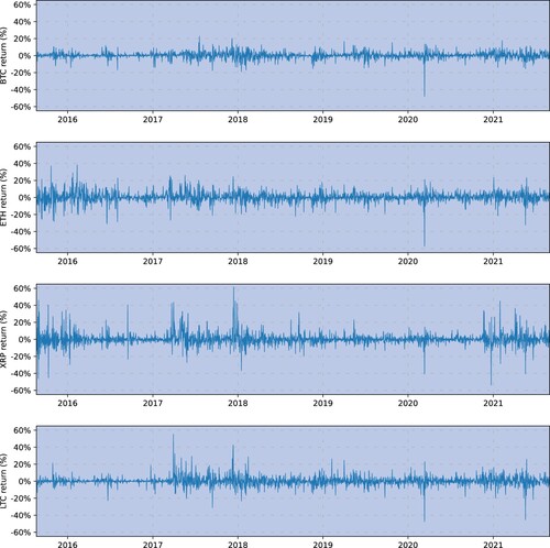
Figure 2. Hourly log returns on bitcoin, ether, ripple and litecoin VWAP USD prices obtained from Cryptocompare. The sample period is 1 January 2021 to 1 July 2021.

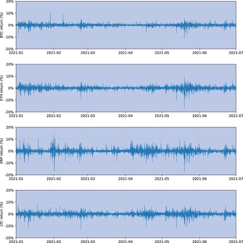
Table 2. Summary statistics of daily log returns on bitcoin (BTC), ether (ETH), ripple (XRP) and litecoin (LTC) VWAP USD prices obtained from Cryptocompare.

	BTC	ETH	XRP	LTC
Mean (%)	0.242%	0.360%	0.228%	0.178%
St. Dev. (% p.a.)	77.1%	121.9%	143.9%	109.1%
Skewness	−0.83	−0.26	0.98	0.54
Ex. Kurtosis	12.07	6.81	11.41	13.04
Min.	−48%	−57%	−54%	−48%
Max.	23%	38%	62%	55%

Notes: The sample period is 20 August 2015 to 31 August 2021. The mean, minimum and maximum are expressed in % and the daily standard deviation is annualized using $\sqrt{365}$.

Table 3. Summary statistics of hourly log returns on bitcoin (BTC), ether (ETH), ripple (XRP) and litecoin (LTC) VWAP USD prices obtained from Cryptocompare.

	BTC	ETH	XRP	LTC
Mean (%)	0.004%	0.026%	0.028%	0.003%
St. Dev. (% p.a.)	104.5%	134.3%	183.6%	148.4%
Skewness	−0.23	−0.80	−0.28	−0.57
Ex. Kurtosis	9.84	8.78	8.10	5.67
Min. (%)	−11%	−17%	−18%	−13%
Max. (%)	12%	9%	13%	8%

Notes: The sample period is 1 January 2021 to 1 July 2021. The mean, minimum and maximum are expressed in % and the hourly standard deviation is annualized using $\sqrt{24\times 365}$.

Table 2 presents summary statistics for the daily log returns for each cryptocurrency over the sample period 20 August 2015 to 31 August 2021. All cryptocurrencies exhibit a relatively small mean, in line with our zero-mean assumption. The skewness is relatively small and can take either sign. The highly significant positive excess kurtosis justifies our assumption for heavy-tailed distributions, captured using Student-t innovations. Table 3 displays summary statistics for the hourly log returns for each cryptocurrency over the sample period January to June 2021. The mean and skewness are again relatively small. As expected, hourly returns are more volatile than daily returns according to the annualized standard deviation, and excess kurtosis is again positive so a heavy-tailed distribution such as the Student-t should be preferable.

We now ask whether the skewness observed in Tables 2 and 3 should warrant the use of the skewed Student-t distribution, such as that defined by Aas and Haff (2006), for the GARCH model innovations. To this end, we estimate a univariate skewed Student-t EGARCH model for each cryptocurrency using the entire daily and hourly sample periods and report the parameter estimates an p-values in Tables 4 and 5. Given the entire sample is very large, for both hourly and daily returns, the estimates of most parameters, including the skewed-t distribution parameter τ, are significant. However, these conditional skewness estimates have a different sign to the unconditional sample skewness observed in Tables 2 and 3. Moreover, the estimates of τ are highly unstable when estimated on rolling sample windows, instead of the entire sample. This suggests that the use of a skewed Student-t distribution can produce a misspecified model, and because it is important to select a robust and easily-estimated GARCH model against which to judge the performance of the simpler, RiskMetrics${}^{\text{TM}}$-type models with ad hoc parameter choices, we do not include the additional source of asymmetry afforded by skew Student-t innovations in our empirical study of asymmetric GARCH models.

Table 4. Parameter estimates and p-values (in parentheses) for each cryptocurrency obtained from the robust standard errors of the univariate skewed-Student-t EGARCH model estimated for the entire daily frequency sample period 20 August 2015—31 August 2021.

	BTC	ETH	XPR	LTC
ω	−0.042 (0.44)	−0.300 (0.00)	−0.291 (0.00)	−0.033 (0.00)
β	0.993 (0.00)	0.946 (0.00)	0.946 (0.00)	0.995 (0.00)
θ	0.048 (0.02)	0.005 (0.80)	0.009 (0.74)	0.033 (0.25)
γ	0.284 (0.00)	0.339 (0.00)	0.445 (0.00)	0.241 (0.00)
ν	2.59 (0.00)	3.28 (0.00)	2.78 (0.00)	2.68 (0.00)
τ	0.93 (0.00)	1.01 (0.00)	1.07 (0.00)	1.03 (0.00)

Notes: The first column denotes the model parameters as defined in Equation (6(6) $\begin{array}{rl}\text{ln}\left({\sigma }_t^2\right)& =\omega +g\left({ϵ}_{t-1}\right)+\text{β}\text{ln}\left({\sigma }_{t-1}^2\right)\\ g\left({ϵ}_t\right)& =\theta {ϵ}_t+\gamma (|{ϵ}_t|-\mathbb{E}\left[|{ϵ}_t|\right]).\end{array}$(6) ), with τ denoting the Student-t distribution's skewness parameter, and the remaining columns denote the parameter estimates and p-values for bitcoin (BTC), ether (ETH), ripple (XRP) and litecoin (LTC).

Table 5. Parameter estimates and p-values (in parentheses) for each cryptocurrency obtained from the robust standard errors of the univariate skewed-Student-t EGARCH model estimated for the entire hourly frequency sample period 1 January 2021—1 July 2021.

	BTC	ETH	XPR	LTC
ω	−0.100 (0.00)	−0.104 (0.00)	−0.140 (0.00)	−0.148 (0.00)
β	0.989 (0.00)	0.988 (0.00)	0.983 (0.00)	0.983 (0.00)
θ	−0.064 (0.00)	−0.043 (0.00)	0.002 (0.87)	−0.046 (0.00)
γ	0.121 (0.05)	0.164 (0.00)	0.250 (0.00)	0.164 (0.00)
ν	4.40 (0.00)	4.82 (0.00)	3.75 (0.00)	5.05 (0.00)
τ	0.94 (0.00)	0.93 (0.00)	0.98 (0.00)	0.95 (0.00)

Notes: The first column denotes the model parameters as defined in Equation (6(6) $\begin{array}{rl}\text{ln}\left({\sigma }_t^2\right)& =\omega +g\left({ϵ}_{t-1}\right)+\text{β}\text{ln}\left({\sigma }_{t-1}^2\right)\\ g\left({ϵ}_t\right)& =\theta {ϵ}_t+\gamma (|{ϵ}_t|-\mathbb{E}\left[|{ϵ}_t|\right]).\end{array}$(6) ), with τ denoting the Student-t distribution's skewness parameter, and the remaining columns denote the parameter estimates and p-values for bitcoin (BTC), ether (ETH), ripple (XRP) and litecoin (LTC).

The asymmetric volatility response refers to a negative correlation between today's return and tomorrow's volatility. Wu (2001), Avramov et al. (2006) and many others since show that this is a well-known feature of traditional financial assets. Regarding cryptocurrency returns, the full-sample daily and hourly frequency Student-t EGARCH parameter estimates shown in Tables 6 and 7 indicate at least one significant volatility response parameter, i.e. θ and γ, as defined in Equation (6(6) $\begin{array}{rl}\text{ln}\left({\sigma }_t^2\right)& =\omega +g\left({ϵ}_{t-1}\right)+\text{β}\text{ln}\left({\sigma }_{t-1}^2\right)\\ g\left({ϵ}_t\right)& =\theta {ϵ}_t+\gamma (|{ϵ}_t|-\mathbb{E}\left[|{ϵ}_t|\right]).\end{array}$(6) ). For the daily data, Table 6 shows that the response size parameter θ is small and positive, and only significant for BTC, but the asymmetry parameter γ is significant for all four cryptocurrencies. For the hourly data, Table 7 shows that the asymmetry parameter γ is again significant for all four cryptocurrencies and the response size parameter θ is large and negative, except for XRP.

Table 6. Parameter estimates and p-values (in parentheses) for each cryptocurrency obtained from the robust standard errors of the univariate Student-t EGARCH model estimated for the entire daily frequency sample period 20 August 2015—31 August 2021.

	BTC	ETH	XPR	LTC
ω	−0.042 (0.31)	−0.302 (0.00)	−0.308 (0.01)	−0.033 (0.00)
β	0.993 (0.00)	0.945 (0.00)	0.943 (0.00)	0.994 (0.00)
θ	0.042 (0.02)	0.006 (0.77)	0.008 (0.76)	0.034 (0.23)
γ	0.270 (0.00)	0.341 (0.00)	0.469 (0.00)	0.242 (0.00)
ν	2.68 (0.00)	3.28 (0.00)	2.75 (0.00)	2.67 (0.00)

Note: The first column denotes the model parameters as defined in Equation (6(6) $\begin{array}{rl}\text{ln}\left({\sigma }_t^2\right)& =\omega +g\left({ϵ}_{t-1}\right)+\text{β}\text{ln}\left({\sigma }_{t-1}^2\right)\\ g\left({ϵ}_t\right)& =\theta {ϵ}_t+\gamma (|{ϵ}_t|-\mathbb{E}\left[|{ϵ}_t|\right]).\end{array}$(6) ) and the remaining columns denote the parameter estimates and p-values for bitcoin (BTC), ether (ETH), ripple (XRP) and litecoin (LTC).

Table 7. Parameter estimates and p-values (in parentheses) for each cryptocurrency obtained from the robust standard errors of the univariate Student-t EGARCH model estimated for the entire hourly frequency sample period 1 January 2021—1 July 2021.

	BTC	ETH	XPR	LTC
ω	−0.100 (0.00)	−0.105 (0.00)	−0.141 (0.00)	−0.147 (0.00)
β	0.989 (0.00)	0.988 (0.00)	0.983 (0.00)	0.983 (0.00)
θ	−0.065 (0.00)	−0.045 (0.00)	0.002 (0.88)	−0.047 (0.00)
γ	0.121 (0.05)	0.163 (0.00)	0.249 (0.00)	0.164 (0.00)
ν	4.39 (0.00)	4.90 (0.00)	3.76 (0.00)	5.08 (0.00)

Note: The first column denotes the model parameters as defined in Equation (6(6) $\begin{array}{rl}\text{ln}\left({\sigma }_t^2\right)& =\omega +g\left({ϵ}_{t-1}\right)+\text{β}\text{ln}\left({\sigma }_{t-1}^2\right)\\ g\left({ϵ}_t\right)& =\theta {ϵ}_t+\gamma (|{ϵ}_t|-\mathbb{E}\left[|{ϵ}_t|\right]).\end{array}$(6) ) and the remaining columns denote the parameter estimates and p-values for bitcoin (BTC), ether (ETH), ripple (XRP) and litecoin (LTC).

Based on daily data in Figure 3 and hourly data in Figure 4 we present θ and γ parameter estimates based on a rolling window of 500 observations. Figure 3 shows that the daily frequency estimates for θ are relaively stable over time, but there is more variation in γ. For instance, during the March 2020 Covid crisis, both BTC and ETH daily returns exhibited an asymmetric volatility response which changed from day to day, due to extreme volatilty following the huge negative returns of over 30%, on 12 March 2020. The most variable parameter estimates are for XRP, which we ascribe to a high-profile lawsuit between Ripple Labs and the SEC.²⁰ Figure 4 covers a different sample, starting only in May 2021. By this time the cryptocurrency markets had matured considerably, and the parameter estimates are much more stable than they are in Figure 3. Again, XRP stands out from the other currencies, with a much smaller θ but a greater γ.

Another intuitive visualization of the volatility response uses the news impact curves defined by Engle and Ng (1993). These are depicted in Figure 5 for daily data and Figure 6 for hourly data. Figure 5 shows symmetric news impact curves at the daily frequency, the greatest impact being for XRP, which is to be expected given the extensive media coverage of the SEC law suit. Figure 6 shows that negative hourly returns have a more pronounced news impact than positive returns of the same magnitude, except for XRP which is more symmetric. We conclude that the cryptocurrency risk profile, as indicated by the shape of the news impact curve, varies considerably across different cryptocurrencies, as well as between daily and hourly returns. The differences observed here confirm a highly idiosyncratic volatility response behaviour even within the four major cryptocurrencies.

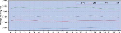
Because we use hourly data, we examine whether the cryptocurrencies in our sample exhibit intra-day volatility periodicity which, if found, can be accounted for as discussed by Andersen and Bollerslev (1997), Stroud and Johannes (2014) and others. To this end, Figure 7 shows the per-hour average in-sample volatility estimates from a univariate Student-t EGARCH model, estimated using the entire sample of hourly data for each cryptocurrency. This shows that only slight variations are observed between different hours-of-day which are very small relative to the overall average volatility levels. More specifically, based on hourly returns bitcoin exhibits an average annualized volatility of 99% but the range of the hour-of-day average volatility between maximum and minimum is only 3.1%. Similarly for ether, the average volatility is 126% and the range is 5.9%, and respectively for ripple 173% and 7.9% and for litecoin 141% and 6.4%. While it may be the case that state-of-the-art volatility models accounting for intra-day volatility periodicity could produce superior results, such complex models may have a limited scope for application by many practitioners, who are likely to favour the simpler models with ad hoc parameter choices that are presented in this paper.

Figure 3. Daily rolling asymmetry parameter estimates for θ (upper panel) and γ (lower panel) as defined in Equation (6(6) $\begin{array}{rl}\text{ln}\left({\sigma }_t^2\right)& =\omega +g\left({ϵ}_{t-1}\right)+\text{β}\text{ln}\left({\sigma }_{t-1}^2\right)\\ g\left({ϵ}_t\right)& =\theta {ϵ}_t+\gamma (|{ϵ}_t|-\mathbb{E}\left[|{ϵ}_t|\right]).\end{array}$(6) ) of the univariate Student-t EGARCH model for bitcoin (BTC, in blue), ether (ETH, in red), ripple (XRP, in green) and litecoin (LTC, in gray). The daily out-of-sample period is 1 January 2019—31 August 2021.

Figure 4. Hourly rolling asymmetry parameter estimates for θ (upper panel) and γ (lower panel) as defined in Equation (6(6) $\begin{array}{rl}\text{ln}\left({\sigma }_t^2\right)& =\omega +g\left({ϵ}_{t-1}\right)+\text{β}\text{ln}\left({\sigma }_{t-1}^2\right)\\ g\left({ϵ}_t\right)& =\theta {ϵ}_t+\gamma (|{ϵ}_t|-\mathbb{E}\left[|{ϵ}_t|\right]).\end{array}$(6) ) of the univariate Student-t EGARCH model for bitcoin (BTC, in blue), ether (ETH, in red), ripple (XRP, in green) and litecoin (LTC, in gray). The hourly frequency out-of-sample period is 1 May 2021—1 July 2021.

Figure 5. News impact curve denoting the volatility response ${\sigma }_t^2$ (vertical axis) to previous-period returns ${ϵ}_{t-1}$ (horizontal axis) for (BTC, in blue), ether (ETH, in red), ripple (XRP, in green) and litecoin (LTC, in gray), obtained from the univariate Student-t EGARCH model estimated for the entire daily frequency sample period 20 August 2015—31 August 2021.

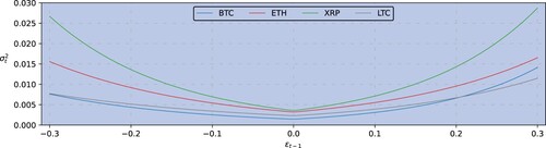
Figure 6. News impact curve denoting the volatility response ${\sigma }_t^2$ (vertical axis) to previous-period returns ${ϵ}_{t-1}$ (horizontal axis) for (BTC, in blue), ether (ETH, in red), ripple (XRP, in green) and litecoin (LTC, in gray), obtained from the univariate Student-t EGARCH model estimated for the entire hourly frequency sample period 1 January 2021—1 July 2021.

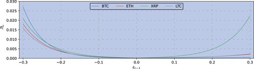
Figure 7. Average in-sample volatility per hour-of-day obtained via the Student-t EGARCH model estimated for the entire hourly frequency sample period 1 January 2021—1 July 2021. In-sample estimated volatility is annualized with a factor of $\sqrt{24\times 365}$ and averaged across the sample for each hour-of-day.

5. Empirical results

We generate out-of-sample, one-period-ahead analysis for bitcoin, ether, ripple and litecoin daily and hourly log returns, comparing the results of the EWMA-type models and more complex GARCH models against the random walk, first backtesting both left- and right-tail VaR and ES in a univariate setting, followed by the results on the univariate and multivariate score-based tests of variance and covariance forecast accuracy. The hourly frequency analysis is then presented in the same order.

We emphasize that the entire ‘raison d’être' for this research is to set ad hoc values for the EWMA parameters. This is because we seek to argue for (or against) setting universal, or at least sector-specific, values for EWMA parameters which are the same for the tens, hundreds (or even thousands) of crypto assets included. This is an important question at this stage in the development of cryptocurrency markets, where some type of extended RiskMetrics${}^{\text{TM}}$ product needs thorough and independent examination. Institutional interest in exploring investment opportunities in a wide variety of coins and tokens is increasing rapidly at the time of writing. However, our parameter selections also need to be sensible. Setting a decay parameter less than about 0.9 would probably be unacceptable to regulators, and the asymmetry parameter should not be so large as to dominate the influence that the realized returns have on volatility. With these comments in mind, we describe how model parameters are selected in more detail below.

5.1. Daily forecasts

Variance and covariance predictions are made daily between 1 January 2017 and 31 August 2021, i.e. for 1,704 daily observations. The benchmark model employs an equally-weighted 30-day moving average. We select precisely 30 days because, although ad hoc, this time period is very commonly used by practitioners and is probably the best suited choice for a single benchmark model. EWMA and AEWMA volatilities and covariances are calculated using two possible values for λ, the RiskMetrics${}^{\text{TM}}$ value 0.94 and a smaller value of 0.925; the AEWMA model further introduces an asymmetry parameter η which is set to 1%, 2% and 3% for left-tail (long positions) VaR/ES forecasting and −1%, −3% and −5% for the right tail (short positions). Results for other choices of η are presented in the Appendix. For instance, Table A5 explores the effect of η on right-tail daily VaR results for short positions and Table A6 does the same, but for left-tail hourly VaR results, for long positions.²¹ The univariate GARCH and multivariate DCC model parameters are estimated using MLE on a fixed-size rolling window with 500 daily log returns, with model parameters are updated on a daily basis.

It is important to note the trade-off between the length of the in-sample/rolling estimation period and the out-of-sample/forecasting period. A longer estimation period might improve the performance of GARCH models for which parameters are estimated via MLE; however, this produces a significantly smaller out-of-sample period and allows for fewer sample points in the forecast accuracy tests. For instance, we have attempted an alternative specification for the GARCH models using a 1,240-day rolling estimation window, but this leaves fewer than 1,000 out-of-sample observations between 1 January 2019 and 31 August 2021. The parameter estimates obtained using the longer estimation window are slightly more stable, but the forecasting results are very similar to those reported here, which use a 500-day estimation window.

Regarding the distribution assumptions, in the random walk benchmark model, crypto cryptocurrency returns are assumed to follow a zero-mean normal distribution. In the EWMA and AEWMA models, a zero-mean location-scale transformed Student-t distribution is used with ad hoc $\nu =6$ degrees of freedom, to produce a heavy-tailed distribution; similarly, a multivariate Student-t with $\nu =6$ is assumed for the joint distribution of bitcoin, ether, ripple and litecoin returns. The GARCH and DCC models also assume a univariate and multivariate Student-t distribution, respectively, where the degrees of freedom parameter is estimated jointly with the model parameters based on the 500-day rolling estimation window.²² GARCH and DCC model estimations and forecasts and also some of the VaR and ES backtesting methods are implemented using the rugarch and rmgarch R packages of Ghalanos (2019, 2020).²³

5.1.1. VaR and ES backtests

We generate VaR and ES one-day-ahead forecasts for bitcoin, ether and ripple at the 1%, 2.5% and 5% significance levels for both the left and right tail of the returns distribution, to assess the ability of each model to capture risk that large negative daily returns present to long positions adequately—and also its ability to capture the risk that large positive daily returns present to short positions. The accuracy of forecast generated by each model is assessed using the tests described in Section 3.2. The results for 1% and 2.5% are presented in Table 8 for the left tail (long positions) and in Table 9 for the right tail (short positions). The results for 5% are less important—at least from the point of view of market regulation—and so are left to the Appendix.

Table 8. Backtesting results for one-day-ahead left-tail 1% and 2.5% VaR forecasts for bitcoin (BTC), ether (ETH), ripple (XRP) and litecoin (LTC), based on an out-of-sample period between 1 January 2017—31 August 2021.

Table 9. Backtesting results for one-day-ahead right-tail 1% and 2.5% VaR forecasts for bitcoin (BTC), ether (ETH), ripple (XRP) and litecoin (LTC), based on an out-of-sample period between 1 January 2017—31 August 2021.

Table 10. Backtesting results for one-day-ahead left-tail 1% and 2.5% ES forecasts for bitcoin (BTC), ether (ETH), ripple (XRP) and litecoin (LTC), based on an out-of-sample period between 1 January 2017—31 August 2021.

Table 11. Backtesting results for one-day-ahead right-tail 1% and 2.5% ES forecasts for bitcoin (BTC), ether (ETH), ripple (XRP) and litecoin (LTC), based on an out-of-sample period between 1 January 2017—31 August 2021.

These results are consistent with most of the findings in the relevant literature as discussed in Section 2. Catania and Grassi (2021) examine GAS model specifications against an EGARCH benchmark for 606 cryptocurrencies and find that the additional modelling complexity introduced by the GAS framework ‘pays off’ for 5% and 1% ES and 5% VaR with increased accuracy, but less so for 1% VaR. In that respect, the results presented in this section for one-day-ahead VaR and ES forecast backtesting are somewhat in agreement with Catania and Grassi (2021) in that introducing additional modelling complexity may sometimes ‘pay off’ in increased forecasting accuracy, especially at lower significance levels; however, we often find that AEWMA specifications are on par with EGARCH in terms of VaR and ES forecasting accuracy even at the 1% significance level.

5.1.2. Score-based tests for variance

We now present the results on univariate and multivariate scores to rank the accuracy of each model for forecasting the one-day-ahead volatility and covariance of bitcoin, ether, ripple and litecoin log returns. The continuous ranked probability score (CRPS) and negatively oriented univariate log score are used to assess univariate density forecasts and joint distribution forecasts are evaluated with the energy score and again with the negatively oriented multivariate log score. Given the parametric distribution assumptions in the models used, i.e. normal for the random walk model and Student-t for the EWMA and GARCH specifications, the one-day-ahead volatility and covariance forecasts fully define the one-day-ahead distribution of log returns for each cryptocurrency and also their joint distribution, allowing for the scores' calculation. All univariate and multivariate scores are calculated using the scoringRules R package of Jordan et al. (2019) combined with custom-written R code.

The CRPS is calculated every day by comparing the realized return with the one-day-ahead log returns density forecast produced by each model and in order to rank the models we average their CRPS over the entire forecasting period. Table 12 reports the results expressed as a percentage of benchmark model's average score which is given in the first row. Due to their negative orientation, relative scores below 100% suggest the possibility that the model is more accurate than the benchmark. We also use the individual scores for every day from each model to perform pair-wise comparisons of forecasting accuracy, by calculating the $t_N$ test statistic of Gneiting and Ranjan (2011) for the hypothesis test of equal forecasting performance as per Equation (30(30) $t_N=\sqrt{N}\left(\frac{{\overline{S}}_N^f-{\overline{S}}_N^g}{{\hat{\sigma }}_N}\right),$(30) ) in Section 3.

Table 12. Average CRPS of one-day-ahead univariate density forecasts for bitcoin (BTC), ether (ETH), ripple (XRP) and litecoin (LTC) daily log returns, based on an out-of-sample period between 1 January 2017—31 August 2021.

	BTC	ETH	XRP	LTC	Energy Score
Benchmark	0.02226	0.03010	0.03436	0.03141	0.06727
tEWMA(0.925)	98.92%	98.79%	98.78%	99.04%	98.47%
tEWMA(0.94)	98.96%	98.87%	98.84%	99.06%	98.57%
tAEWMA(0.925, 1%)	99.18%	98.87%	98.76%	99.08%	98.93%
tAEWMA(0.925, 2%)	99.74%	99.07%	99.02%	99.27%	99.18%
tAEWMA(0.925, 3%)	100.89%	99.50%	99.62%	99.75%	99.66%
tAEWMA(0.925,−1%)	98.99%	98.75%	98.69%	99.04%	98.88%
tAEWMA(0.925,−3%)	101.17%	99.52%	99.39%	99.72%	99.57%
tAEWMA(0.925,−5%)	107.00%	102.19%	101.75%	102.10%	102.07%
tAEWMA(0.94, 1%)	99.23%	98.96%	98.80%	99.10%	99.02%
tAEWMA(0.94, 2%)	99.80%	99.17%	99.09%	99.32%	99.23%
tAEWMA(0.94, 3%)	100.97%	99.62%	99.70%	99.83%	99.73%
tAEWMA(0.94,−1%)	99.04%	98.83%	98.72%	99.06%	98.90%
tAEWMA(0.94,−3%)	101.22%	99.61%	99.45%	99.76%	99.62%
tAEWMA(0.94,−5%)	107.04%	102.27%	101.84%	102.15%	102.16%
tGARCH	98.85%	97.99%	97.57%	98.79%	98.35%
tEGARCH	98.70%	97.95%	97.69%	98.60%	102.19%

Notes: As the CRPS and energy score are negatively oriented and produce positive values, a relative score lower than 100% indicates outperformance of the benchmark. For the random walk benchmark model the average CRPS is reported outright and the average scores of the remaining models are expressed as a percentage of the benchmark's score. The EWMA, AEWMA and GARCH models are based on a Student-t distribution assumption and the degrees of freedom for EWMA and AEWMA are set to the ad hoc $\nu =6$ and for GARCH the degrees of freedom are estimated via MLE. The right-most column reports the average energy scores for one-day-ahead joint density forecasts of all four coins. For the tGARCH and tEGARCH models, the energy scores refer to the ADCC multivariate model. The relative energy scores for the DCC multivariate model are 98.43% for tGARCH and 102.14% for tEGARCH.

As shown in Table 12, most models outperform the benchmark although none of them achieve an average CRPS lower than 97% and the $t_N$ test for a significant difference between the highest and lowest average scores is always below 0.15, so the null hypothesis of equal forecasting performance is never rejected at 5%. This suggests that all models examined, including our very simple benchmark, produce equally inaccurate one-day-ahead density forecasts for the returns of bitcoin, ether, ripple and litecoin. This result extends the findings of Catania and Grassi (2021) that equal forecasting performance between an EGARCH benchmark model and more complex GAS models is the most common outcome.

The energy score is calculated by drawing 10,000 random samples from the forecast joint density of log returns produced by each model, based on the corresponding realized returns.²⁶ Again for comparison purposes, each score is averaged over the entire forecasting period. The right-hand column of Table 12 reports the outright average energy score for the benchmark model and the average energy scores of all other models are again expressed relative to the benchmark's average score. Again, most models outperform the benchmark but the $t_N$ test statistic for equal forecasting performance cannot reject the null hypothesis even at 5% and even when testing the model having lowest energy score versus the benchmark. So all models produce equally accurate one-day-ahead covariance forecasts—none of the multivariate parametric models perform any better than the simplest benchmark.

As with the CRPS and energy scores, the univariate and multivariate log scores are calculated via the corresponding one-day-ahead predictive densities based on the realized returns and the volatility and covariance forecasts produced by each model. Again, the average log score is expressed outright for the benchmark in Table 13 and relative to the benchmark score for all other models. Table 13 shows that all models produce a higher relative score compared with the benchmark, contrary to the findings for the CRPS and energy score. However, this is because we employ the negatively oriented log score which produces negative average scores in all cases; consequently, a lower (i.e. more negative) log score is higher in magnitude but still indicates a better forecast. Therefore, the results shown in Table 13 are consistent with the findings for the CRPS and energy scores, in that all models outperform the benchmark. Moreover, the $t_N$ test statistic for equal forecasting performance applied to the log scores cannot reject the null hypothesis that the models produce the same scores, even at 5%. In other words, based on the logarithmic score results and well as the CRPS and energy score results, all models produce equally accurate one-day-ahead variance forecasts and similarly, none of the multivariate parametric models perform any better than the benchmark.

Table 13. Average log score of one-day-ahead univariate density forecasts for bitcoin (BTC), ether (ETH), ripple (XRP) and litecoin (LTC) daily log returns.

	BTC	ETH	XRP	LTC	MV LogS
Benchmark	−1.62193	−1.42004	−1.26143	−1.32140	−6.52492
tEWMA(0.925)	114.55%	108.55%	117.21%	114.34%	124.45%
tEWMA(0.94)	114.53%	108.46%	117.20%	114.35%	124.60%
tAEWMA(0.925, 1%)	113.92%	108.33%	117.47%	114.34%	123.11%
tAEWMA(0.925, 2%)	113.09%	108.12%	117.06%	114.12%	122.67%
tAEWMA(0.925, 3%)	111.41%	107.50%	115.72%	113.23%	121.90%
tAEWMA(0.925,−1%)	114.58%	108.81%	117.77%	114.51%	123.28%
tAEWMA(0.925,−3%)	111.13%	107.72%	116.67%	113.49%	122.01%
tAEWMA(0.925,−5%)	103.71%	103.33%	111.53%	109.16%	119.54%
tAEWMA(0.94, 1%)	113.87%	108.24%	117.46%	114.31%	123.42%
tAEWMA(0.94, 2%)	112.99%	107.96%	116.94%	113.98%	122.98%
tAEWMA(0.94, 3%)	111.28%	107.29%	115.53%	113.02%	122.22%
tAEWMA(0.94,−1%)	114.47%	108.71%	117.79%	114.50%	123.62%
tAEWMA(0.94,−3%)	111.00%	107.55%	116.46%	113.36%	122.36%
tAEWMA(0.94,−5%)	103.63%	103.18%	111.26%	109.01%	119.94%
tGARCH	115.03%	110.47%	121.21%	115.38%	125.15%
tEGARCH	115.56%	110.54%	121.30%	116.13%	120.68%

Notes: For the random walk benchmark model the average log score is reported outright and the average scores of the remaining models are expressed as a percentage of the benchmark's score. As the negatively oriented version of the log score is used which produces negative values, a relative score higher than 100% indicates outperformance of the benchmark. The EWMA, AEWMA and GARCH models are based on a Student-t distribution assumption and the degrees of freedom for EWMA and AEWMA are set to the ad hoc $\nu =6$ and for GARCH the degrees of freedom are estimated via MLE. The right-most column reports the average multivariate log scores (MV LogS) for one-day-ahead joint density forecasts of all four coins. For the tGARCH and tEGARCH models, the multivariate log scores refer to the ADCC multivariate model. The relative multivariate log scores for the DCC multivariate model are 125.08% for tGARCH and 120.63% for tEGARCH.

5.2. Hourly forecasts

We now present the same analysis performed on a more recent sample of hourly bitcoin, ether, ripple and litecoin log returns between 1 May 2021 00:00 UTC and 1 July 2021 00:00 UTC. The benchmark model forecasts are based on an equally-weighted 72-hour moving average; the EWMA and AEWMA forecasts are again produced with λ set to 0.925 and 0.94 but the AEWMA η parameter is now set to lower values i.e. to 0.7%, 0.8% and 0.9% for long positions and −0.2% and 0.2% for short positions, to be in line with smaller hourly returns.²⁷ GARCH models are calibrated using a rolling estimation window of 4 months, i.e. 2,882 hourly observations. The same distribution assumptions as for the daily frequency analysis are followed, i.e. we use normal innovations for the benchmark, a Student-t distribution with $\nu =6$ for the EWMA and AEWMA models, and for the GARCH models the degrees of freedom parameter is estimated with the other model parameters via MLE.

5.2.1. VaR and ES backtesting

The hourly 1% left-tail (long position) VaR forecast results show in Table 14, suggest that the AEWMA models are the only ones that produce fewer than the expected 14.65 exceedances for 1% VaR.²⁸ For these models the CC test's null hypothesis of no clustering in exceedences is accepted even at the 10% level of significance. By comparison, the tEGARCH models are in the yellow zone and the standard tGARCH forecasts are in fact not considered accurate at all. The right-tail (short position) hourly 1% VaR backtesting results which are presented in Table 15 appear to favour the simple model specifications even more; for instance, the 1% right-tail VaR forecasts produced by the symmetric tEWMA models are considered accurate based on both the traffic light and CC tests, and even the simplest random walk benchmark model produces accurate 1% VaR forecasts for bitcoin and ripple, which is on a par with the more complex GARCH specifications.

Table 14. Backtesting results for one-hour-ahead left-tail 1% and 2.5% VaR forecasts for bitcoin (BTC), ether (ETH), ripple (XRP) and litecoin (LTC). For each asset, the first column denotes the models used, where the EWMA, AEWMA and GARCH models are based on a Student-t distribution assumption and the degrees of freedom for EWMA and AEWMA are set to the ad hoc $\nu =6$ and for GARCH the degrees of freedom are estimated via MLE.

Table 15. Backtesting results for one-day-ahead left-tail 1% and 2.5% VaR forecasts for bitcoin (BTC), ether (ETH), ripple (XRP) and litecoin (LTC), based on an out-of-sample period between 1 January 2017—31 August 2021.

Table 16. Backtesting results for one-hour-ahead left-tail 1% and 2.5% ES forecasts for bitcoin (BTC), ether (ETH), ripple (XRP) and litecoin (LTC).

Table 17. Backtesting results for one-hour-ahead right-tail 1% and 2.5% ES forecasts for bitcoin (BTC), ether (ETH), ripple (XRP) and litecoin (LTC).

5.2.2. Score-based tests for variance

The average CPRS based on the hourly volatility forecasts for each cryptocurrency, and the energy score for the covariance forecasts, are presented in Table 18. Again, the average score for the benchmark is given in the first row and the subsequent rows present each model's average score relative to the benchmark score. Again, the benchmark yields a higher average score (indicating a poorer performance) than almost every other model. The tEGARCH model yields the lowest average CRPS for all cryptocurrencies except ripple and the ADCC-tGARCH yields the lowest average energy score. Importantly, and similar to the discussion of our daily frequency analysis, the test of equal forecasting performance does not distinguish between the models: the $t_N$ test statistic between the highest and lowest average scores is always below 0.45, so the null hypothesis of equal forecasting performance is accepted e.g. at the 5% and 10% significance levels based on both the CRPS for each cryptocurrency and on the energy score.³⁰ This suggests that the equal forecasting performance identified previously based on the average scores of daily returns density forecasts also holds at the hourly frequency: i.e. all models examined, even the random walk benchmark, are considered equally accurate regarding one-hour-ahead volatility and covariance forecasts for the returns of bitcoin, ether, ripple and litecoin.

Table 18. Average CRPS of one-hour-ahead univariate density forecasts for bitcoin (BTC), ether (ETH), ripple (XRP) and litecoin (LTC) hourly log returns.

	BTC	ETH	XRP	LTC	Energy Score
Benchmark	0.00613	0.00858	0.00920	0.00890	0.01788
tEWMA(0.925)	99.25%	99.13%	98.44%	99.25%	98.67%
tEWMA(0.94)	99.19%	99.11%	98.43%	99.22%	98.69%
tAEWMA(0.925, 0.2%)	99.15%	99.04%	98.40%	99.16%	98.90%
tAEWMA(0.925, 0.7%)	99.85%	99.01%	98.70%	99.16%	99.06%
tAEWMA(0.925, 0.8%)	100.32%	99.12%	98.89%	99.28%	99.27%
tAEWMA(0.925, 0.9%)	100.94%	99.30%	99.13%	99.46%	99.46%
tAEWMA(0.925,−0.2%)	99.36%	99.20%	98.49%	99.32%	99.05%
tAEWMA(0.94, 0.2%)	99.10%	99.02%	98.40%	99.14%	98.88%
tAEWMA(0.94, 0.7%)	99.87%	99.04%	98.74%	99.20%	99.14%
tAEWMA(0.94, 0.8%)	100.35%	99.17%	98.94%	99.33%	99.21%
tAEWMA(0.94, 0.9%)	100.97%	99.35%	99.19%	99.52%	99.50%
tAEWMA(0.94,−0.2%)	99.30%	99.17%	98.49%	99.28%	99.03%
tGARCH	98.91%	98.82%	98.04%	98.89%	98.68%
tEGARCH	98.56%	98.63%	98.10%	98.73%	98.62%

Notes: For the random walk benchmark model the average CRPS is reported outright and the average scores of the remaining models are expressed as a percentage of the benchmark's score. As the CRPS and energy score are negatively oriented and produce positive values, a relative score lower than 100% indicates outperformance of the benchmark. The EWMA, AEWMA and GARCH models are based on a Student-t distribution assumption and the degrees of freedom for EWMA and AEWMA are set to the ad hoc $\nu =6$ and for GARCH the degrees of freedom are estimated via MLE. The right-most column reports the average energy scores for one-day-ahead joint density forecasts of all four coins. For the tGARCH and tEGARCH models, the energy scores refer to the ADCC multivariate model. The relative energy scores for the DCC multivariate model are 98.71% for tGARCH and 98.60% for tEGARCH.

Similarly, the average univariate and multivariate log scores are shown in Table 19. The average log scores of all models are greater in magnitude than the benchmark's average score which, as mentioned previously, indicates a better performance than the benchmark due to the negative sign of all average scores. As before, the test of equal forecasting performance indicates an equal performance across all models, for all assets and also for the multivariate log score, even at the 5% and 10% significance levels. It therefore appears that both the CPRS/energy score and univariate/multivariate log scores indicate an equal forecasting performance in all cases, for hourly data just as they do for daily data.

Table 19. Average log score of one-hour-ahead univariate density forecasts for bitcoin (BTC), ether (ETH), ripple (XRP) and litecoin (LTC) hourly log returns.

	BTC	ETH	XRP	LTC	MV LogS
Benchmark	−3.06639	−2.74713	−2.67047	−2.71165	−13.18273
tEWMA(0.925)	102.49%	102.85%	104.16%	102.88%	104.44%
tEWMA(0.94)	102.61%	102.91%	104.25%	102.94%	104.68%
tAEWMA(0.925, 0.2%)	102.67%	102.99%	104.27%	103.04%	104.17%
tAEWMA(0.925, 0.7%)	102.17%	103.11%	104.01%	103.10%	103.97%
tAEWMA(0.925, 0.8%)	101.76%	102.97%	103.77%	102.93%	103.82%
tAEWMA(0.925, 0.9%)	101.24%	102.77%	103.48%	102.70%	103.65%
tAEWMA(0.925,−0.2%)	102.42%	102.80%	104.13%	102.83%	104.11%
tAEWMA(0.94, 0.2%)	102.75%	103.03%	104.34%	103.07%	104.41%
tAEWMA(0.94, 0.7%)	102.15%	103.05%	103.97%	103.03%	104.17%
tAEWMA(0.94, 0.8%)	101.72%	102.91%	103.73%	102.85%	104.03%
tAEWMA(0.94, 0.9%)	101.20%	102.70%	103.42%	102.61%	103.86%
tAEWMA(0.94,−0.2%)	102.53%	102.86%	104.21%	102.89%	104.37%
tGARCH	103.08%	103.28%	104.80%	103.39%	104.97%
tEGARCH	103.39%	103.48%	104.81%	103.57%	104.91%

Notes: For the random walk benchmark model the average log score is reported outright and the average scores of the remaining models are expressed as a percentage of the benchmark's score. As the negatively oriented version of the log score is used which produces negative values, a relative score higher than 100% indicates outperformance of the benchmark. The EWMA, AEWMA and GARCH models are based on a Student-t distribution assumption and the degrees of freedom for EWMA and AEWMA are set to the ad hoc $\nu =6$ and for GARCH the degrees of freedom are estimated via MLE. The right-most column reports the average multivariate log scores (MV LogS) for one-day-ahead joint density forecasts of all four coins. For the tGARCH and tEGARCH models, the energy scores refer to the ADCC multivariate model. The relative log scores for the DCC multivariate model are 104.97% for tGARCH and 104.91% for tEGARCH.

6. Conclusions

The standard RiskMetrics${}^{\text{TM}}$ EWMA methodology fails to provide the industry standard of 99% coverage for VaR and ES of cryptocurrencies, at least when the decay parameter λ is 0.94, this being equal to the value set for returns on traditional financial assets. However, a lower value than 0.94 may be appropriate for cryptocurrencies because their volatility tends to be more highly reactive to market shocks and also less persistent, and reducing λ has precisely this effect. Having said this, we have not been able to produce the required level of coverage with other values for λ, lower, or higher than 0.94, even when innovations are drawn from a Student-t distribution.

What is important is that the EWMA model includes an asymmetry in volatility response. That is, volatility increases more following a negative return than it does following a positive return of the same magnitude. It is simple to do this by introducing another parameter η to the EWMA model, and with this modification we refer to the model as AEWMA, or more precisely as the AEWMA$(\lambda ,\eta ,\nu )$ model, where ν is the degrees of freedom in the Student-t innovations. We explore the values of λ, η and ν that do provide 99% coverage, with the same parameter values for all cryptocurrencies. This way, we may also use these values in a multivariate framework without concern for non-positive definiteness of the covariance matrix.

Our empirical results show that this simple, constant parameter AEWMA model performs as well as the fully-calibrated Student-t EGARCH models, which require at least several hundred observations in-sample, before any backtesting begins—and even more observations are required for calibration of their multivariate equivalents if these are to be employed in portfolio optimization. Running several state-of-the-art VaR and Expected Shortfall backtests over a five-year period at the daily frequency, and using several thousands of observations at the hourly frequency, we find that a coverage level of 99% for VaR and ES is easy to achieve for long or short positions on all cryptocurrencies considered is possible, provided we have the right parameter choices. Although a small improvement in coverage is obtainable using sophisticated GARCH models, the incremental returns to this effort are unlikely to be seen as attractive by industry practitioners. Also our univariate and multivariate score-driven tests for variance and covariance indicate no significant improvements in average scores which would warrant a ranking for GARCH models above our simple asymmetric extension for a RiskMetrics${}^{\text{TM}}$ type EWMA.

Disclosure statement

No potential conflict of interest was reported by the author(s).

Notes

1 A relevant Scopus search yields 342 papers published between 2015 and early 2022 in Economics, Econometrics, Finance, Business, Management or Accounting journals and 131 of these papers were published in 2021 or early 2022. These results are produced with the following Scopus search query: TITLE-ABS-KEY((‘bitcoin’ OR ‘Bitcoin’ OR ‘ethereum’ OR ‘ether’ OR ‘Ethereum’ OR ‘Ether’ OR ‘cryptocurrency’ OR ‘cryptocurrencies’ OR ‘cryptoasset’ OR ‘crypto asset’ OR ‘crypto’ OR ‘digital currency’ OR ‘digital asset’ OR ‘crypto currency’) AND (‘GARCH’ OR ‘EWMA’ OR ‘Value at Risk’ OR ‘VaR’ OR ‘Value-at-Risk’ OR ‘ES’ OR ‘Expected shortfall’ OR ‘volatility’ OR ‘covariance’ OR ‘variance’) AND (‘model*’ OR ‘forecast*’ OR ‘estimat*’)) AND (LIMIT-TO(DOCTYPE, ‘ar’)) AND (LIMIT-TO(SUBJAREA, ‘ECON’) OR LIMIT-TO(SUBJAREA, ‘BUSI’)).

2 Note that the above refers to relatively unsophisticated retail investors that maintain unhedged positions in cryptocurrencies; it does not apply e.g. to investors or market makers that partially or completely hedge their positions with derivatives.

3 The OKEx blog even mentions that ‘VaR is useful for calculating the maximum expected loss on an investment’, which is a highly inaccurate and misleading interpretation.

4 These so-called ‘ghost features’ have been recognized in traditional financial markets for decades—see, for instance, Section IV.2.10.2 in Alexander (2008).

5 The optimal sample size is highly dependent on the characteristics of the data. For cryptocurrency univariate volatility modelling, between one and two years of data have been a common choice. Much larger samples are required for multivariate model calibrations to be stable over rolling or expanding windows.

6 Historical data for the above cryptocurrencies are obtained from the following sources: blockchain.com, Binance, Bitstamp, Bloomberg, Brave New Coin, Coindesk, Coinmarketcap, Cryptocompare, Gemini and Kraken.

7 See for example, [MAR31.12], [MAR31.23] and [MAR31.26] of Minimum capital requirements for market risk.

8 Implementation of these models commonly employs maximum likelihood estimation (MLE), which is the simplest method of multivariate optimization. Markov chain Monte Carlo (MCMC) has also been applied to regime-switching GARCH models, but only at the univariate level. We note that Tiwari et al. (2019) use the cross-entropy method of Rubinstein (1997) for calculating the marginal likelihood, again in a univariate model.

9 For this reason, in the following the term GARCH always means GARCH(1,1), unless otherwise stated.

10 There is much support for the zero-mean assumption as already discussed in Section 2. For instance, Köchling et al. (2020) find that GARCH model specifications for bitcoin returns that have zero mean are very often included in the model confidence set.

11 Note that the ‘raw’ ER test consists of using the raw residuals which are not divided by the estimated standard deviation. This version of the ER test is suggested by Bayer and Dimitriadis (2020), who argue that ‘the test using the standardized ER is in fact a joint backtest for the triple VaR, ES and volatility, whereas the test using the raw ER is a joint backtest for the pair VaR and ES’.

12 It would also be possible to assess the accuracy of volatility and covariance forecasts via a loss function such as the mean absolute error of point forecasts but, as mentioned by Gneiting and Ranjan (2011), the CRPS may be regarded as an extension of the mean absolute error for density forecasts, instead of point forecasts.

13 The null hypothesis that the VaR model is ‘specified correctly’ implies a joint hypothesis that the time series of VaR exceedance indicators $X_t^{\text{VaR}}\left(\alpha \right)$ is independent and identically distributed (i.i.d.) and that the proportion of realized VaR exceedances is equal to the VaR significance level α. Note that the above definition holds for both left- and right-tail VaR, as exceedances are defined respectively based on the 100α% left and right tail of the distribution.

14 Note that in the case of the VaR traffic light backtest, the binomial distribution is commonly used and is (almost) as easy to work with as the normal. We choose the normal approximation of the binomial distribution to ensure the easiest possible application of our ad hoc methodology, and also for consistency with the ES traffic light backtest where we use the asymptotic normal distribution approximation as suggested by Costanzino and Curran (2018). The approximation of the binomial distribution with the normal is considered accurate based on the rule-of-thumb that both $N\alpha$ and $N(1-\alpha )$ should be greater than 5, which is the case for the analysis presented in Section 5, as we use N = 1, 704 in the daily frequency analysis, N = 1, 465 in the hourly frequency and $\alpha =1\mathrm{\%}$, $2.5\mathrm{\%}$ and $5\mathrm{\%}$.

15 As the number of realized VaR exceedances $x^{\text{VaR}}$ over the forecasting period is a realization of the random variable $X_N^{\text{VaR}}\left(\alpha \right)$ defined in Equations (16(16) $X_N^{\text{VaR}}\left(\alpha \right)=\sum _{t=1}^N{X}_t^{\text{VaR}}\left(\alpha \right).$(16) ) and (17(17) $X_N^{\text{VaR}}\left(\alpha \right)\sim \mathcal{N}(N\alpha ,N\alpha (1-\alpha )).$(17) ), the probability of obtaining $x^{\text{VaR}}$ or fewer VaR exceedances is given as: $P\left(X_N^{\text{VaR}}\right(\alpha )\le x^{\text{VaR}})=P(\frac{X_N^{\text{VaR}}\left(\alpha \right)-N\alpha }{\sqrt{N\alpha (1-\alpha )}}\le \frac{x^{\text{VaR}}-N\alpha }{\sqrt{N\alpha (1-\alpha )}})=\mathrm{\Phi }\left(z\right)$, where $z\sim \mathcal{N}(0,1)$.

16 As in the case of the traffic light backtest, the conditional coverage test definitions hold for both left- and right-tail VaR, as exceedances are defined respectively based on the 100α% left and right tail of the distribution.

17 As noted previously for VaR, the null hypothesis that the ES model is ‘specified correctly’ implies a joint hypothesis that the time series of ES generalized exceedance indicators $X_t^{\text{ES}}\left(\alpha \right)$ is i.i.d. and that for all $p\in [0,\alpha ]$, the probability of VaR exceedances is $P(r_t\le -{\text{VaR}}_t(p\left)\right)=p$ for the left tail and $P(r_t\ge {\text{VaR}}_t(p\left)\right)=p$ for the right tail.

18 Note that the derivation described in Costanzino and Curran (2015) yields the asymptotic distribution of our Equation (22(22) $X_N^{\text{ES}}\left(\alpha \right)\sim \mathcal{N}(\frac{1}{2}N\alpha ,N\alpha \left(\frac{4-3\alpha }{12}\right)).$(22) ), whereas the distribution's variance in equation (17) of Costanzino and Curran (2018) is mistakenly omitting a factor of N. Regarding the accuracy of the normal approximation, Clift et al. (2016) perform a simulation study and find that the approximation is accurate for a forecasting period of length N = 250; this confirms that the normal approximation is fit for use in our analysis, as we use forecasting periods that include over 1, 000 observations.

19 For instance, the live-streamed implied volatility index for bitcoin typically exceeds 100%, which is more than five times greater than the S&P 500 volatility index, VIX.

20 For example, since December 2020 and thus during our entire sample for hourly data, Ripple Labs has been engaged in a high-profile law suit, filed by the U.S. Securities and Exchange Commission (SEC), and still ongoing at the time of writing. There is now a major class action by XRP coin holders claiming that the SEC law suit has had a highly detrimental effect on XRP returns.

21 As mentioned previously, note that the ad hoc value choices for the asymmetry parameter should be large enough to improve forecasting accuracy but also small enough to avoid a dominating influence of realized returns on volatility.

22 The daily returns exhibit some asymmetry in their sample statistics, but not always in the same direction, as shown in Table 2. But the asymmetric model specifications can still capture this characteristic to some extent even with the symmetric distribution assumption that we use. Also, the choice of a symmetric distribution simplifies the process of modelling the joint density for the returns of bitcoin, ether, ripple and litecoin.

23 The multivariate EWMA model is implemented using the RiskPortfolios R package of Ardia et al. (2017), and the remaining EWMA and AEWMA specifications and also the traffic light backtesting methodology are implemented using custom-written R code.

26 These are produced using the mvnfast R package of Fasiolo (2016).

27 Additional testing for other AEWMA η parameter choices is reported in the Appendix.

28 The expected number of VaR exceedances for 1% VaR is calculated based on (17(17) $X_N^{\text{VaR}}\left(\alpha \right)\sim \mathcal{N}(N\alpha ,N\alpha (1-\alpha )).$(17) ) using N = 1, 465 and $\alpha =1\mathrm{\%}$.

30 As discussed in Section 3, the null hypothesis for the test of equal forecasting performance is that $t_N=0$, tested against the two-sided alternative that $t_N\ne 0$, where $t_N\sim \mathcal{N}(0,1)$. Therefore, if the null hypothesis is to be rejected e.g. at the 5% or 10% significance levels, then $t_N$ should be outside the 2.5% or 5% right- and left-tail critical values which are respectively $\pm 1.96$ and $\pm 1.64$.

Appendix

Table A1. Backtesting results for one-day-ahead left- (long position) and right-tail (short position) 5% VaR forecasts for bitcoin (BTC), ether (ETH), ripple (XRP) and litecoin (LTC), based on an out-of-sample period between 1 January 2017 and 31 August 2021.

Table A2. Backtesting results for one-day-ahead left- (long position) and right-tail (short position) 5% ES forecasts for bitcoin (BTC), ether (ETH), ripple (XRP) and litecoin (LTC), based on an out-of-sample period between 1 January 2017 and 31 August 2021.

Table A3. Backtesting results for one-hour-ahead one-day-ahead left- (long position) and right-tail (short position) 5% VaR forecasts for bitcoin (BTC), ether (ETH), ripple (XRP) and litecoin (LTC), based on an out-of-sample period between 1 May 2021 and 1 July 2021.

Table A4. Backtesting results for one-hour-ahead one-day-ahead left- (long position) and right-tail (short position) 5% ES forecasts for bitcoin (BTC), ether (ETH), ripple (XRP) and litecoin (LTC), based on an out-of-sample period between 1 May 2021 and 1 July 2021.

Table A5. Backtesting of daily left-tail 1% VaR for a short position on bitcoin (BTC), ether (ETH), ripple (XRP) and litecoin (LTC).

Table A6. Backtesting of hourly left-tail 1% VaR on bitcoin (BTC), ether (ETH), ripple (XRP) and litecoin (LTC).

Table A7. Backtesting of hourly right-tail 1% VaR on bitcoin (BTC), ether (ETH), ripple (XRP) and litecoin (LTC).

References

- Aas, K. and Haff, I.H., The generalized hyperbolic skew Student-t distribution. J. Financ. Econom., 2006, 4(2), 275–309.
- Acereda, B., Leon, A. and Mora, J., Estimating the expected shortfall of cryptocurrencies: An evaluation based on backtesting. Finance Res. Lett., 2020, 33, 101181.
- Aielli, G.P., Dynamic conditional correlation: On properties and estimation. J. Bus. Econ. Stat., 2013, 31(3), 282–299.
- Al-Khazali, O., Bouri, E. and Roubaud, D., The impact of positive and negative macroeconomic news surprises: Gold versus bitcoin. Econ. Bulletin, 2018, 38(1), 373–382.
- Al-Yahyaee, K., Mensi, W., Al-Jarrah, I., Hamdi, A. and Kang, S., Volatility forecasting, downside risk, and diversification benefits of bitcoin and oil and international commodity markets: A comparative analysis with yellow metal. North American J. Econ. Finance, 2019, 49, 104–120.
- Alexander, C., Market Risk Analysis: Value-at-Risk Models, 2008 (John Wiley and Sons: Chichester).
- Alexander, C. and Dakos, M., A critical investigation of cryptocurrency data and analysis. Quant. Finance, 2020, 20(2), 173–188.
- Andersen, T.G. and Bollerslev, T., Intraday periodicity and volatility persistence in financial markets. J. Empir. Finance, 1997, 4(2-3), 115–158.
- Ardia, D., Bluteau, K. and Rüede, M., Regime changes in bitcoin GARCH volatility dynamics. Finance Res. Lett., 2019, 29, 266–271.
- Ardia, D., Boudt, K. and Gagnon-Fleury, J.-P., RiskPortfolios: Computation of risk-based portfolios in R. J. Open Source Softw., 2017, 2(10), 171.
- Avramov, D., Chordia, T. and Goyal, A., The impact of trades on daily volatility. Rev. Financ. Stud., 2006, 19(4), 1241–1277.
- Basel Committee, Supervisory framework for the use of backtesting in conjunction with the internal models approach to market risk capital requirements. Basel Committee on Banking Supervision, 1996. Available at: https://www.bis.org/publ/bcbs22.htm.
- Basel Committee, Fundamental review of the trading book: A revised market risk framework. Basel Committee on Banking Supervision, 2012. Available at: https://www.bis.org/publ/bcbs219.htm.
- Baur, D., Dimpfl, T. and Kuck, K., Bitcoin, gold and the US dollar: A replication and extension. Finance Res. Lett., 2018, 25, 103–110.
- Bauwens, L. and Storti, G., A component GARCH model with time varying weights. Stud. Nonlinear Dyn. Econom., 2009, 13(2), 1–33.
- Bayer, S. and Dimitriadis, T., Regression-based expected shortfall backtesting. J. Financ. Econom., 2020, 20, 437–471.
- Bazán-Palomino, W., Bitcoin and its offspring: A volatility risk approach. In Advanced Studies of Financial Technologies and Cryptocurrency Markets, edited by L. Pichl, C. Eom, E. Scalas and T. Kaizoji, pp. 233–256, 2020 (Springer: Singapore).
- Bollerslev, T., Generalized autoregressive conditional heteroskedasticity. J. Econom., 1986, 31(3), 307–327.
- Bonello, A. and Suda, D., Volatility regime analysis of bitcoin price dynamics using Markov-switching GARCH models. In Proceedings of the European Simulation and Modelling Conference 2018, pp. 213–218, 2018 (Department of Industrial Systems Engineering and Product Design, University of Gent: Gent). https://biblio.ugent.be/publication/8593929
- Bouoiyour, J. and Selmi, R., Commodity price uncertainty and manufactured exports in Morocco and Tunisia: Some insights from a novel GARCH model. Econ. Bulletin, 2014, 34(1), 220–233.
- Bouoiyour, J. and Selmi, R., Bitcoin: A beginning of a new phase? Econ. Bulletin, 2016, 36(3), 1430–1440.
- Bouri, E., Molnar, P., Azzi, G., Roubaud, D. and Hagfors, L., On the hedge and safe haven properties of bitcoin: Is it really more than a diversifier? Finance Res. Lett., 2017, 20, 192–198.
- Bovaird, C., Bitcoin price volatility reached a 14-month high in June. Forbes, 2021. Available at: https://bit.ly/3zLZtXw.
- Caporale, G. and Zekokh, T., Modelling volatility of cryptocurrencies using Markov-switching GARCH models. Res. Int. Bus. Finance, 2019, 48, 143–155.
- Cappiello, L., Engle, R.F. and Sheppard, K., Asymmetric dynamics in the correlations of global equity and bond returns. J. Financ. Econom., 2006, 4(4), 537–572.
- Catania, L. and Grassi, S., Forecasting cryptocurrency volatility. Int. J. Forecast., 2021, 38, 878–894.
- Catania, L., Grassi, S. and Ravazzolo, F., Forecasting cryptocurrencies under model and parameter instability. Int. J. Forecast., 2019, 35(2), 485–501.
- Chen, C.W., Watanabe, T. and Lin, E.M., Bayesian estimation of realized GARCH-type models with application to financial tail risk management. Econom. Statistics, 2021. Article in Press. https://www.sciencedirect.com/science/article/pii/S2452306221000484
- Christoffersen, P., Evaluating interval forecasts. Int. Econ. Rev. (Philadelphia), 1998, 39(4), 841–862.
- Chu, J., Chan, S., Nadarajah, S. and Osterrieder, J., GARCH modelling of cryptocurrencies. J. Risk Financ. Manage., 2017, 10(4), 17.
- Clift, S., Costanzino, N. and Curran, M., Empirical performance of backtesting methods for expected shortfall. SSRN Discussion Paper 2618345, 2016.
- Corbet, S., Lucey, B., Peat, M. and Vigne, S., Bitcoin futures: What use are they? Econ. Lett., 2018, 172, 23–27.
- Costanzino, N. and Curran, M., Backtesting general spectral risk measures with application to expected shortfall. SSRN Discussion Paper 2514403, 2015.
- Costanzino, N. and Curran, M., A simple traffic light approach to backtesting expected shortfall. Risks, 2018, 6(1), 2.
- Creal, D., Koopman, S.J. and Lucas, A., Generalized autoregressive score models with applications. J. Appl. Econom., 2013, 28(5), 777–795.
- Diebold, F.X. and Mariano, R.S., Comparing predictive accuracy. J. Bus. Econ. Stat., 1995, 13(3), 253–263.
- Ding, Z., Granger, C. and Engle, R., A long memory property of stock market returns and a new model. J. Empir. Finance, 1993, 1(1), 83–106.
- Dyhrberg, A., Bitcoin, gold and the dollar—A GARCH volatility analysis. Finance Res. Lett., 2016, 16, 85–92.
- Engle, R., Dynamic conditional correlation: A simple class of multivariate generalized autoregressive conditional heteroskedasticity models. J. Bus. Econ. Stat., 2002, 20(3), 339–350.
- Engle, R., Ghysels, E. and Sohn, B., Stock market volatility and macroeconomic fundamentals. Rev. Econ. Stat., 2013, 95(3), 776–797.
- Engle, R. and Manganelli, S., CAViaR: Conditional autoregressive value at risk by regression quantiles. J. Bus. Econ. Stat., 2004, 22(4), 367–381.
- Engle, R.F., Focardi, S.M. and Fabozzi, F.J., ARCH/GARCH models in applied financial econometrics. In Encyclopedia of Financial Models, edited by F.J. Fabozzi, 2012 (John Wiley and Sons). https://doi.org/10.1002/9781118182635.efm0062
- Engle, R.F. and Kroner, K.F., Multivariate simultaneous generalized ARCH. Econ. Theory., 1995, 11(1), 122–150.
- Engle, R.F. and Lee, G., A Long-Run and Short-Run Component Model of Stock Return Volatility, 1999 (Oxford University Press: Oxford).
- Engle, R.F. and Ng, V.K., Measuring and testing the impact of news on volatility. J. Finance, 1993, 48(5), 1749–1778.
- Fantazzini, D. and Zimin, S., A multivariate approach for the simultaneous modelling of market risk and credit risk for cryptocurrencies. J. Ind. Bus. Econ., 2020, 47(1), 19–69.
- Fasiolo, M., An introduction to mvnfast. R package version 0.1.6., 2016.
- Fissler, T. and Ziegel, J.F., Higher order elicitability and Osband's principle. Ann. Statist., 2016, 44(4), 1680–1707.
- Ghalanos, A., Rmgarch: Multivariate GARCH models. R package version 1.3-7., 2019.
- Ghalanos, A., Rugarch: Univariate GARCH models. R package version 1.4-4., 2020.
- Glosten, L.R., Jagannathan, R. and Runkle, D.E., On the relation between the expected value and the volatility of the nominal excess return on stocks. J. Finance, 1993, 48(5), 1779–1801.
- Gneiting, T. and Raftery, A.E., Strictly proper scoring rules, prediction, and estimation. J. Am. Stat. Assoc., 2007, 102(477), 359–378.
- Gneiting, T. and Ranjan, R., Comparing density forecasts using threshold- and quantile-weighted scoring rules. J. Bus. Econ. Stat., 2011, 29(3), 411–422.
- Guesmi, K., Saadi, S., Abid, I. and Ftiti, Z., Portfolio diversification with virtual currency: Evidence from bitcoin. Int. Rev. Financ. Anal., 2019, 63, 431–437.
- Hansen, P., Lunde, A. and Nason, J., The model confidence set. Econometrica, 2011, 79(2), 453–497.
- Hansen, P.R., Huang, Z. and Shek, H.H., Realized GARCH: A joint model for returns and realized measures of volatility. J. Appl. Econom., 2012, 27(6), 877–906.
- Hattori, T., A forecast comparison of volatility models using realized volatility: Evidence from the bitcoin market. Appl. Econ. Lett., 2020, 27(7), 591–595.
- Hentschel, L., All in the family: Nesting symmetric and asymmetric GARCH models. J. Financ. Econ., 1995, 39(1), 71–104.
- Higgins, M.L. and Bera, A.K., A class of non-linear ARCH models. Int. Econ. Rev. (Philadelphia), 1992, 33(1), 137–158.
- Jordan, A., Krüger, F. and Lerch, S., Evaluating probabilistic forecasts with scoringRules. J. Stat. Softw., 2019, 90(12), 1–37.
- Katsiampa, P., Volatility estimation for bitcoin: A comparison of GARCH models. Econ. Lett., 2017, 158, 3–6.
- Köchling, G., Schmidtke, P. and Posch, P., Volatility forecasting accuracy for bitcoin. Econ. Lett., 2020, 191, 108836.
- Kratz, M., Lok, Y.H. and McNeil, A.J., Multinomial VaR backtests: A simple implicit approach to backtesting expected shortfall. J. Bank. Finance, 2018, 88, 393–407.
- Kupiec, P., Techniques for verifying the accuracy of risk measurement models. J. Derivatives, 1995, 3(2), 73–84.
- Liu, W., Semeyutin, A., Lau, C.K.M. and Gozgor, G., Forecasting value-at-risk of cryptocurrencies with riskmetrics-type models. Res. Int. Bus. Finance, 2020, 54, 101259.
- Longerstaey, J. and Spencer, M., RiskMetrics—Technical Document. J. P. Morgan/Reuters, 1996.
- López-Cabarcos, M., Pérez-Pico, A., Piñeiro Chousa, J. and Šević, A., Bitcoin volatility, stock market and investor sentiment. Are they connected? Finance Res. Lett., 2020, 38, 101399.
- Maciel, L., Cryptocurrencies value-at-risk and expected shortfall: Do regime-switching volatility models improve forecasting? Int. J. Finance Econ., 2021, 26(3), 4840–4855.
- Matheson, J.E. and Winkler, R.L., Scoring rules for continuous probability distributions. Manage. Sci., 1976, 22(10), 1087–1096.
- Matkovskyy, R., Jalan, A. and Dowling, M., Effects of economic policy uncertainty shocks on the interdependence between bitcoin and traditional financial markets. Q. Rev. Econ. Finance, 2020, 77, 150–155.
- McMillan, D.G. and Kambouroudis, D., Are riskmetrics forecasts good enough? Evidence from 31 stock markets. Int. Rev. Financ. Anal., 2009, 18(3), 117–124.
- McNeil, A. and Frey, R., Estimation of tail-related risk measures for heteroscedastic financial time series: An extreme value approach. J. Empir. Finance, 2000, 7(3-4), 271–300.
- Mincer, J.A. and Zarnowitz, V., The evaluation of economic forecasts. In Economic Forecasts and Expectations: Analysis of Forecasting Behavior and Performance, pp. 3–46, 1969 (NBER). https://econpapers.repec.org/bookchap/nbrnberbk/minc69-1.htm
- Nekhili, R. and Sultan, J., Jump-driven risk model performance in cryptocurrency market. Int. J. Financ. Stud., 2020, 8(2), 1–18.
- Nelson, D.B., Conditional heteroskedasticity in asset returns: A new approach. Econometrica, 1991, 59(2), 347–370.
- Pafka, S. and Kondor, I., Evaluating the riskmetrics methodology in measuring volatility and value-at-risk in financial markets. Physica A: Statist. Mechan. Appl., 2001, 299(1-2), 305–310.
- Patton, A.J., Volatility forecast comparison using imperfect volatility proxies. J. Econom., 2011, 160(1), 246–256.
- Rubinstein, R.Y., Optimization of computer simulation models with rare events. Eur. J. Oper. Res., 1997, 99(1), 89–112.
- Schwert, G.W., Stock volatility and the crash of '87. Rev. Financ. Stud., 1990, 3(1), 77–102.
- Segnon, M. and Bekiros, S., Forecasting volatility in bitcoin market. Ann. Finance, 2020, 16, 435–462.
- Silahli, B., Dingec, K., Cifter, A. and Aydin, N., Portfolio value-at-risk with two-sided Weibull distribution: Evidence from cryptocurrency markets. Finance Res. Lett., 2021, 38, 101425.
- Sosa, M., Ortiz, E. and Cabello, A., Bitcoin conditional volatility: GARCH extensions and Markov switching approach. Int. Finance Rev., 2019, 20, 201–219.
- Stavroyiannis, S., Value-at-risk and related measures for the bitcoin. J. Risk Finance, 2018, 19(2), 127–136.
- Stroud, J.R. and Johannes, M.S., Bayesian modeling and forecasting of 24-hour high-frequency volatility. J. Am. Stat. Assoc., 2014, 109(508), 1368–1384.
- Takahashi, M., Watanabe, T. and Omori, Y., Volatility and quantile forecasts by realized stochastic volatility models with generalized hyperbolic distribution. Int. J. Forecast., 2016, 32(2), 437–457.
- Takahashi, M., Watanabe, T. and Omori, Y., Forecasting daily volatility of stock price index using daily returns and realized volatility. Econom. Statist., 2021. Article in Press. https://www.sciencedirect.com/science/article/pii/S2452306221000964
- Tiwari, A., Kumar, S. and Pathak, R., Modelling the dynamics of bitcoin and litecoin: GARCH versus stochastic volatility models. Appl. Econ., 2019, 51(37), 4073–4082.
- Troster, V., Tiwari, A., Shahbaz, M. and Macedo, D., Bitcoin returns and risk: A general GARCH and GAS analysis. Finance Res. Lett., 2019, 30, 187–193.
- Trucíos, C., Forecasting bitcoin risk measures: A robust approach. Int. J. Forecast., 2019, 35(3), 836–847.
- Trucíos, C., Hotta, L.K. and Ruiz, E., Robust bootstrap forecast densities for GARCH returns and volatilities. J. Stat. Comput. Simul., 2017, 87(16), 3152–3174.
- Trucíos, C. and Taylor, J., A comparison of methods for forecasting value-at-risk and expected shortfall of cryptocurrencies. ResearchGate Working Paper, 2022.
- Tse, Y.K. and Tsui, A.K.C., A multivariate generalized autoregressive conditional heteroscedasticity model with time-varying correlations. J. Bus. Econ. Stat., 2002, 20(3), 351–362.
- Vidal-Tomás, D. and Ibañez, A., Semi-strong efficiency of bitcoin. Finance Res. Lett., 2018, 27, 259–265.
- Wang, J.-N., Liu, H.-C., Chiang, S.-M. and Hsu, Y.-T., On the predictive power of ARJI volatility forecasts for bitcoin. Appl. Econ., 2019, 51(44), 4849–4855.
- Wu, G., The determinants of asymmetric volatility. Rev. Financ. Stud., 2001, 14(3), 837–859.
- Zakoian, J.-M., Threshold heteroskedastic models. J. Econ. Dyn. Control, 1994, 18(5), 931–955.