Advancing cervical cancer diagnosis and screening with spectroscopy and machine learning

ABSTRACT

Introduction

In the UK alone, the incidence of cervical cancer is increasing, hence an urgent need for early and rapid detection of cancer before it develops. Spectroscopy in conjunction with machine learning offers a disruptive technology that promises to pick up cancer early as compared to the current diagnostic techniques used.

Areas covered

This review article explores the different spectroscopy techniques that have been used for the analysis of cervical cancer. Along with the extensive description of spectroscopic techniques, the various machine learning techniques are also described as well as the applications that have been explored in the diagnosis of cervical cancer. This review delimits the literature specifically associated with cervical cancer studies performed solely with the use of a spectroscopy technique, and machine learning.

Expert opinion

Although there are several methods and techniques to detect cervical cancer, the clinical sector requires to introduce new diagnostic technologies that help improve the quality of life of patients. These innovative technologies involve spectroscopy as a qualitative method and machine learning as a quantitative method. In this article, both the techniques and methodologies that allow and promise to be a new screening tool for the detection of cervical cancer are covered.

KEYWORDS:

• Machine learning
• cervical cancer
• HPV (human papillomavirus)
• vibrational spectroscopy
• diagnosis
• screening

1. Introduction

In the UK only, the cervical cancer rate is approximately 10 in every 100,000 women [1]]. In 2020, 604,000 new cases and 342,000 deaths were estimated [2], with approximately 90% of the 260,000 annual deaths occurring in less-developed regions [3] A range of factors are related to this disparity, including reduced screening and HPV vaccine availability due to limited resources [4,5], reduced medical availability requiring travel to a major city for screening [6], a lack of female doctors, and cultural conservatism [7]. Even in higher-income countries such as the UK and USAA, the World Health Organization’s aim to eradicate cervical cancer is challenged by either patients avoiding current diagnosis methods [8], or lack of participation by marginalized communities [9].

Persistent human papillomavirus (HPV), especially the high-risk HPV-16 and HPV-18, is known to be essential for cervical cancer to occur [10]. Risk factors for HPV include smoking, HIV, low socioeconomic level, multiple sexual partners, and because HPV is a sexually transmitted infection, sexual intercourse before the age of 16 [10]. The current approach to cervical cancer screening is a Pap smear test, an invasive procedure causing lowered participation [8]. Further diagnosis can be carried out by white light colposcopy with a sensitivity of ~ 96% but a specificity of ~ 48% [11]. A biopsy is the gold standard for diagnosis but is further invasive and can be impractical for patients with several suspicious lesions [11]. Developing new approaches could provide improvements in the overall accuracy of cervical cancer diagnosis, as well as a more accessible sample collection.

Spectroscopy, a range of techniques for investigating the molecular compositions, has been used for a wide range of cervical cancer diagnosis applications including the distinction of the cancerous from normal cells [11], separation of precancerous stages [12], classification of cervical cancer grades [13], and different types of cervical cancer [14]. However, spectroscopy also provides the opportunity to detect HPV and cervical cancer through the analysis of biofluids, potentially reducing the invasiveness of sample collection and making screening more accessible in rural areas. Biofluid collection can also be carried out during times of imposed social distancing, such as the COVID-19 pandemic, where in-person testing was disrupted [15]. Fiber-optic Raman provides the opportunity for in vivo testing (section 4) [11], speeding diagnosis when paired with machine learning. The increasing developments in spectroscopy machine learning and enlargement of datasets are therefore hoped to speed the steady adoption [16] of clinical spectroscopy.

It should be emphasized that machine learning is a vast area of research, with spectroscopy analysis largely focused on supervised and unsupervised learning (section 2). The application of deep learning in cervical cancer diagnosis with spectroscopy [17] is an area of development when compared to the wider use of computer vision with other methods [18–22]. However, the increased number of studies, especially in studies applying supervised learning in section 4, has resulted in techniques for processing samples, the beginning of consensus in approach, a specified goal described by Baker et al. community [16]. Collection and analysis method consensus would provide standardized approaches to produce larger, potentially multi-center datasets that would more accurately emulate the real-world screening and diagnosis of cervical cancer. This review article does not focus on a deep explanation of machine learning theory, we recommend and encourage the reader to consult the references from this article, and to perform further research related to machine learning theory.

2. Machine learning methods

2.1. Unsupervised learning

Unsupervised learning is an approach to analyze multivariate data by the application of different clustering methods [23]. The following sub-sections will briefly explain the most common methods used in unsupervised machine learning for spectral data.

2.1.1. Principal Component Analysis (PCA)

The aim of PCA consists of reducing the dimensions of the input dataset [24,25]. For datasets obtained from spectroscopy it is common to have more than 3000 variables, and PCA focuses on compressing the dataset to assist their interpretation. Overall, the dimension reduction process of PCA consists of obtaining the covariance matrix of the data set, followed by the calculation of Eigen stuff (eigenvectors and eigenvalues) which will bring the PCs as an outcome (Figure 1a). The researcher must be able to distinguish how many PCs to use by using the elbow method when plotting the eigenvalues or explained variance [24,25].

Figure 1. a) Cluster analysis. An overview of how the dimension reduction occurs. 1. The original matrix may have n number of columns with n variables. 2. In the example a matrix of 5 dimensions is depicted, and then exemplified that it’s not possible to plot a 5 dimension plot. 3. Depicts the step of covariance matrix creation. 4. The covariance matrix selection gives way to the eigenstuff calculation, the eigenstuff includes the eigenvectors (λ), and eigenvalues (ν), which together build the principal components. 5. Principal components now can be compared against each other, creating a 2D plot. 6. The PCs create now a reduced matrix in comparison with the input matrix, allowing an easier interpretability. b) Dendrogram of a hierarchical cluster analysis. The Dendrogram depicts where the leaves and nodes are localized. The HCA was able to find two clusters, green and red. c) K means example. The image shows where the random centroids were placed after the final iteration. The distance border, commonly Euclidean distance, helps to the data points to find the closest distance to the closest centroid.

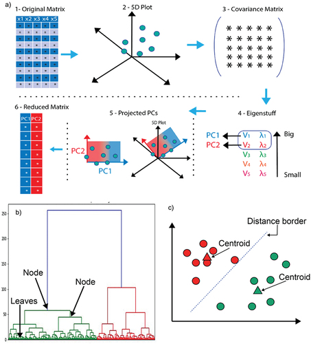
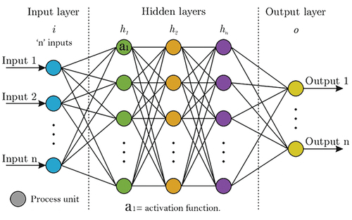
Figure 2. Overall structure of an ANN. Each ANN consists of different process units, and layers. The activation function works within each process unit.

2.1.2. Hierarchical cluster analysis (HCA)

HCA is visualized by using dendrograms which are a representation of the linkage distance (similarity) that exists between sub-sets. The nodes of the dendrogram depict a breakdown of the similarity among the data set culminating in the leaves which are the individual clustering of the data points (Figure 1b). HCA can be categorized in two ways, agglomerative clustering and divisive clustering. HCA may employ four different methods to measure the similarity in a data set; Ward’s linkage, average linkage, complete linkage, and single linkage [24,26].

2.1.3. K-means

K-means can be considered as a simple unsupervised method to implement in spectroscopy. The K-means algorithm generates random centroids among the datasets which serve as reference points for the cluster assignment (Figure 1c). The k-means clustering algorithm computes the distance that exists between each individual data point and the centroid to the group the data points with similar distances. The selection of the best k value can be obtained through statistical measures, such as the silhouette coefficient, and elbow curve method by calculating the sum of squared distances [27–29]. K-means can be used in conjunction with PCA to aid the interpretability of the data [30].

2.2. Supervised learning

Supervised learning is a type of machine learning in which a model is trained on a labeled dataset to make predictions or classifciations on new, or unseen data. Table 1, at the end of this section, provides an overall summary of the most common supervised models used in machine learning.

Table 1. Highlights of the supervised models presented. This table aims to provide an overall overview of advantages and disadvantages of the machine learning supervised methods.

Model	Advantages	Disadvantages
LDA	Considers the different scales and correlations between variables. LDA uses information from the features to create a new axis which in turn minimizes the variance and maximizes the class distance of the two variables.	Number of variables needs to be less than number of samples. Data must be normal distributed. Does not consider variance of each class.
PLS-DA	No need to apply PCA prior to PLS. Able to handle more descriptive variables.	Linear regression is a limitation. Number of variables needs to be less than number of samples. Does not consider variance of each class.
SVM	The algorithm works well when the class separation is clear. SVM is effective with high-dimensional spaces. Efficient when number of dimensions is greater than number of samples.	Large datasets not effective when using SVM (Large data sets definition is relative and arguably, can be bigger than 100K columns). Not performs well when classes overlap.
KNN	Easy implementation Low parameters used. Can be used for classification or regression problems. Multiclass prediction allowed.	The efficiency of the algorithm diminishes as the number of data, predictors, and variables increase.
LR	Implementation is not difficult. Easy to interpret. Allows multiclass predictions.	If the observations are less than the features the model will overfit. Linearity assumption is a limitation.
RF	Reduces data overfitting. Can be used for classification or for regression. It is not necessary to normalize data.	Requires high computational sources to create big sets of decision trees. Can take a lot of time to train the data, since it combines several decision trees.
NNs	NNs can learn by themselves. NNs can detect non-linear relationships among the data. Efficient for medical classifications.	Requires efficient and quick computational resources. The processing units can be perceived as a black box, and not being able to detect problems. Prone to overfitting.
EMs	The prediction may improve since it considers different supervised models. Predictions can be stable in bagging method. Boosting reduces bias of the model. Stacking tends to improve accuracy and keeping variance and bias low.	Interpretation can be difficult. Ensemble models can be hard to construct. Training of data can be difficult to perform.

2.2.1. Linear Discriminant Analysis (LDA)

LDA aims to find new axes that maximize the variance between the classes, whilst minimizing the variance within the classes, producing clusters that can be observed in reduced dimensions [31]. Using LDA to transform the data onto new dimensions reduces the curse of dimensionality [32], making comprehensible visualizations possible. Classification is made possible by the application of a discrimination rule, potential rules include maximum likelihood, Fisher’s linear discriminant rule, and Baye’s discriminant rule, the most common. Baye’s discriminant rule produces a probability field for each class, predicting samples that are in the class for which they have the greatest probability value. A limitation of LDA is the assumption that features used to train the model to have a normal (Gaussian) distribution [33]. Training datasets for LDA are also required to be balanced (have similar numbers of samples in each class) for the algorithm to perform well. Training datasets for LDA are also considered to improve through balanced configuration for the algorithm to perform well. Interestingly, altering datasets for balancing purposes (rebalancing) has been shown to adversely affect results [34].

2.2.2. Partial least squares discriminant analysis (PLS-DA)

Partial least squares (PLS) carried out a linear transform on the dataset, reducing the data dimensions similarly to PCA, where both PLS and PCA produce score plots (latent variables and principal components, respectively), and loadings plots [35]. The differences between PLS and PCA include the PLS production of weightings plots and the axes criteria [36]. The latent variables PLS rotate the data onto relates to the between-group variability [37] in the independent variables X and dependent variables Y, whereas principal components show the maximum variance within a dataset X [36]. The Y-block provides a key difference between PLS and PCA, directing the transformation, making PLS a supervised technique (where PCA is unsupervised). Partial least squares-discriminant analysis (PLS-DA), which is PLS used for discrimination (classification), combines the use of binary encoded dummy variables to categorize new samples into different classes [37]. For example, in a binary classification problem (aiming to distinguish two sample types or classes) the first class (cancerous) is encoded as 0 and the second (healthy) is encoded as 1. If the PLS-DA determines a new sample to have a value above 0.5, it would predict that sample to be healthy, being closer to the healthy classes encoded value of 1.

2.2.3. Support Vector Machines (SVMs)

SVMs determine hyperplanes that separate the data into classes, which can either be two classes (binary classification) or more (multi-class classification) [38]. The advantages of SVMs include working well when the number of features is larger than the number of observations. SVMs are highly adaptable, with different kernels (functions) that can be used for different data types, for example, the linear kernel for linear data and the polynomial kernel for the non-linear kernel [38]. SVMs can also be used for both classification and regression analysis. Hyperparameters such as C and gamma (γ) can be used to tailor the model to a specific analysis. C applies a penalty to misclassified samples, reducing the decision boundary as C increases in size to avoid misclassification and the incurred penalty [38]. The kind of hyperparameter that may need to be optimized depends on the kernel, for a linear kernel, only C is required to be optimized. Another commonly used kernel is the radial bias function (RBF) kernel [39], for the RBF kernel, the hyperparameter gamma can also be optimized. Gamma influences area of influence for a sample, when gamma is lower the area of influence is larger, associating more samples. The outcome of altering hyperparameters is that the model can be optimized for different applications. For example, if a study requires high sensitivity for an application such as cancer screening, where further testing can identify false negatives, hyperparameters can be tailored for a sensitivity-focused SVM.

2.2.4. K- Nearest Neighbors (KNN)

KNN is a simple and easy-to-understand algorithm, based on the principle that similar samples will be ‘closer’ to each other when compared along all dimensions (features) of the dataset [40]. Each sample is a point in an n-dimensional space (where n is the number of dimensions/features), with clusters visualized by coloring each point based on the samples label. Classification of new samples is carried out by plotting the new sample in the n-dimensional space, measuring the distance from that sample to a number ‘K’ of nearest samples, and assigning it (classifying it) to the class with the greatest number of samples within those samples [40]. For example, if K = 1, the new sample will be classified as being the same as the sample that is closest to it. If K = 15, the fifteen nearest samples will be determined, and the sample assigned to the class with the greatest contribution within those fifteen. If there is a tied number within the fifteen, say, the classes with five samples each, the class can either be assigned at random or excluded [41]. The advantages of KNN are simplicity and ease of use. It is relatively simple to understand that samples that have been measured as like each other would probably be similar in general [40,42]. As each classification is made by measuring the distance to each other observations, there is no training time, potentially speeding analysis. The limitations of KNN are linked to the increased computational cost incurred during the calculation of distances for datasets with large numbers of observations or features (or both) [40], KNN, therefore, performs best for low-feature datasets [40,42].

2.2.5. Logistic Regression (LR)

LR carries out binary classification by converting input values to scaled positions between 0 and 1 with a logistic sigmoid function [43], producing a probability of the sample being either one class (relating to 0) or the other (relating to 1). Classification is generally carried out based on whether the probability of the sample is <0.5 (closer to 0) or >0.5 (closer to 1). An advantage of logistic regression is its capacity for feature selection [44]. Features without evidence of importance can be removed from further analysis, leaving features that can be investigated further. For spectroscopy, a key limitation lies in the need for more observations (spectra) than features (wavelengths) to avoid overfitting. A common rule of thumb is to use 10 observations per feature, resulting in a 1000 wavenumber spectrum requiring the collection of 10,000 spectra if the entire spectrum was included (although this is not always the case [45]. Logistic regression, therefore, requires significant dimension reduction through PCA or feature selection if oversampling is to be avoided for spectral studies.

2.2.6. Random Forest (RF)

RFs are ensemble algorithms that combine decision trees [46]. Decision trees are simple and robust algorithms that form branches based on criteria within nodes [47]. The decisions can be based on categorical or continuous data [47], in spectroscopy, it could be a wavelength intensity or principal component score. The nodes are ordered relating to how well they distinguish the observations (samples), with the first providing the greatest classification power [47]. The number of nodes and layers in a decision tree can continue until the data can no longer be split with the available features, producing highly interpretable and easily understood results [47]. Decision trees have significant advantages, including the ability to analyze samples with missing values, not requiring scaled data, or making assumptions about the features. The main limitation of decision trees is overfitting. Decision trees are easy to overfit as the tree grows, with a key indicator being nodes without further division (leaves) containing only a small number of samples. To counter the overfitting limitation of decision trees, many small decision trees can be combined into a random forest [46]. RF algorithms are similarly robust concerning the data being used, but avoid overfitting by combining the classification power of many small classifiers [48].

2.2.7. Neural Networks

Neural networks are computational models which can classify or organize datasets. Schematically, a neural network model consists of different processing units which are connected and run in parallel. These processing units aim to mimic a neuron from a biological brain where a series of decisions occur. A neural network may consist of an ‘n’ number of layers, each with an ‘n’ number of process units (Figure 2) [24,49,50]. The number of layers depends on the type of neural network; shallow or deep neural network. Whereas the number of processing units depends on the model input defined by the user. A shallow neural network may have between 5 and 10, but this number may differ [24,49,50]. The product of the mathematical process that occurs on each processing unit is classified by the activation function. In other words, the activation function is responsible for characterizing the data by classes, or groups [24,49,50]. Based on the author’s experience, in spectroscopy it is recommended to use ReLu, sigmoid, or ReLu activation functions, for binary or multiclass predictions, however, this is subject to the users’ criteria.

2.2.8. Ensemble methods

In comparison with the previous supervised learning methods, ensemble methods provide a different approach and its principal objective is to combine the prediction of different supervised learning algorithms to improve robustness over a single estimator [51,52].

There is no finite number of estimators to combine to obtain the ideal model. Therefore, the flexibility of this method allows different alternatives to be explored. Ensemble methods can be classified into three classes: bagging, stacking, and boosting [51,52].

Bagging is the short term for bootstrap aggregating. In essence, bagging works by iterating different decision tree algorithms and averaging the predictions performed by it to arrive at a consensual output [51–53]. For example, let us suppose we have a binary classification where healthy and not healthy samples are being predicted and an ensemble method with decision trees is being used. The model will generate X number of trees, and each individual decision tree will have its own outcome, then the model will vote for the most frequent output and consider it as the definitive answer. Furthermore, bagging is not limited to decision trees, random forest, and extremely randomized trees methods can also be used for developing a bagging ensemble method [52,53].

Stacking is similar to bagging. The only difference relies on the use of different models that are not decision trees, random forests, or extremely randomized trees. Instead, other supervised models are used, such as SVM, LR, KNN, etc. A stacking ensemble method will generate X different supervised models and will average the output of each model to get a consensual result [51–53].

Differently, from bagging and stacking, boosting ensemble methods instead of only evaluating individual models within the ensemble method, each model will function as ‘training raw material’ to improve the following model. Overall, the objective of a boosting ensemble method is to train on a previous existent model within the ensemble method, iterate each model to the following models to correct predictions of prior models, and finally obtain a consensual prediction based on a blend of weighted average models [51–53].

3. Method comparison of featured studies

The articles cited in this review have a wide disparity in the methods the researchers use in their studies. This variety of methods indicates that there is a lack of standardization or consensus under which samples should be collected, prepared, and analyzed by machine learning. This section allows the reader to have a broad overview, according to the literature, of the selection of these different methods based on the sample type.

The only consensus that researchers follow in the analysis of biological samples for cervical cancer is that samples need to be collected directly from patients and require strict informed consent issued by the authority under which the researchers fall.

The literature cited substantially differs in the selection of study groups (Figure 3a). Some of the studies recruit control group patients (healthy, with cervicitis, or benign tumors), patients diagnosed with cancer, and patients with precancer [13,14,17,20,54–60]. Other studies are limited to comparing only between healthy patients and patients diagnosed with cancer [61–68]. However, it has been found that some authors prefer to study only between abnormal or precancer vs. cancer samples [69,70], whereas the majority of the authors study healthy patients vs. a precancer grade, either high grade, or low grade, or abnormal cells not considered cancer [11,12,56,71–82]. Furthermore, there were few studies where patients or samples were only diagnosed with human papillomavirus independent of the cancer status and compared against healthy or non-HPV-detected patients or samples [83–87]. The sample group selection does not necessarily follow a specific procedure, since it varies according to the spectroscopic method. Nonetheless, what is important to highlight from the above-mentioned patient recruitment, is that researchers rarely use a balanced sample input, normally in proportion 1:1 which is essential for machine learning analysis. Most of the studies go beyond a 1:1 sample proportion, having up to a 1:10 sample proportion which will bring bias to machine learning models (Figure 3d).

Figure 3. Method comparison found on the literature. a: Class selection. b: Spectra collection according to the spectroscopy method. c: Consent form as unique consensus. d: Reported ML balance. E: Reported ML split. F: Metrics reported and metrics recommended for ML analysis.

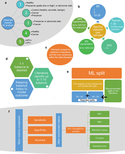
As previously mentioned, another aspect on which no consensus can be reached between the spectroscopy and machine learning analysis is the number of spectra collected for subsequent supervised analysis (Figure 3b). For IR spectroscopy 1, 3, 10–20, spectra are collected per sample [17,58,61,66,73,83,84,86,88,89]. Raman spectroscopy has been found to be one of the most used spectroscopy techniques to analyze cancer samples, however the spectra collection ranges between 1–30 spectra per sample [11–13,19,54,56,62–65,69,70,72,74–76,87,90–92], being 3–8 the most common spectra collection range per sample, however this is not well established. In contrast the studies where diffuse reflectance spectroscopy (DRS) is being used, only 1 to 2 spectra are collected per sample [20,57,81]. The minority of spectroscopy techniques such as mass spectrometry (MS), and nuclear magnetic resonance (NMR), use 50 to 1200 m/z [85], and 64 or 128 free induction decays (FUD) into 32 k data points [59,68], respectively.

When creating machine learning models, it is necessary to split the data set into training and test sets (Figure 3E). Normally, it is recommended that either 70% training and 30% testing, or 80% training and 20% testing, should be used [52,53]. However, it was found that the majority of the literature does not specify, whereas the ones that report it [57,77,81,88,92] range between the 70–30, or 80–20 split, with the exception of the study performed by Traynor et al. (2022) [12] that reported a data split of 95% training and 5% testing.

Finally, as part of the evaluation, model’s metrics are necessary (Figure 3F). Overall, the most used metrics for predictive models are specificity, sensitivity, and accuracy of prediction. However, positive predictive value (PPV), negative predictive value (NPV), receiver operating characteristic/area under the curve (ROC/AUC) plots, standard error of prediction (opposite to accuracy of prediction), and F1 score, can be alternative metrics to strengthen the analysis.

4. Spectroscopy and machine learning for cervical cancer diagnosis

4.1. Biofluids

Undoubtedly, the diagnosis of cervical cancer using spectroscopy and machine learning has a huge area of opportunity to be further exploited. In vibrational spectroscopy alone, the application of these tools together promises to lead to the development of a new diagnostic technique for cervical cancer. Scientists have explored analyzing biofluids in conjunction with Raman and infrared spectroscopy, due to their ease of acquisition, as well as having the major advantage of being minimally invasive. However, it seems that studies are still limited to exploring blood as an essential biofluid for the diagnosis of cervical cancer.

A study from 2022, performed by Ma et al. (2022) [17], demonstrated to successfully implement a promising cervical cancer diagnosis using Infrared spectroscopy and convolutional NNs, using blood serum. This study has an interesting scope since it includes a variety of patients (cancer, precancer, and patients with benign tumors as the control group). The study included no more than 40 patients, and no less than 20 patients per group, making it slightly imbalanced, but sufficient to perform predictions. The complexity of convolutional NNs allows their model to have a good performance given the reduced amount of collected samples. This model provided a great accuracy of prediction between 83.3% and 91.3% for all the groups analyzed, having an average of 87.2% prediction accuracy. The researchers undoubtedly proved that the implantation of their model might be exploited for cancer diagnosis, however, further research should be considered.

Similarly, González-Solís et al. (2014) [91] implemented, Raman spectroscopy in blood serum samples, as a different approach for cervical cancer diagnosis. However, their research was limited to a more simplistic machine learning application, PCA-LDA. Although they could identify unique spectral biomarkers attributed to cancer, such as glutathione at 446 cm⁻¹, and 1404 cm⁻¹ they successfully showed a unique PCA discrimination from their samples, nonetheless the study requires robustness on their metrics.

On the other hand, still under the blood analysis scope, Feng et al. (2013) [64] analyzed blood plasma using surface-enhanced Raman spectroscopy (SERS), with PCA-LDA as a machine learning model. Their model only included healthy patients and patients with cervical cancer. Their study showed a sensitivity of 96.7%, and a specificity of 92%, with adequate discrimination. However, the major issue to consider is the feasibility of applying SERS in the clinical setup, given the additional steps that are required to prepare samples. In contrast, another study in blood plasma from Raja et al. (2019) [67], also using Raman spectroscopy and PCA-LDA, achieved a sensitivity of 94.4% and a specificity of 96.7%, slightly higher in comparison with the study of Feng et al. (2013). However, it is important to consider that Raja et al. (2019) [67] collected spectra from 18 patients, whilst Feng et al. (2013) [64] analyzed spectra from 110 patients. Interestingly, Feng et al. (2013) [64] analyzed a wider spectral region between 1750–350 cm⁻¹, in comparison with Raja et al. (2019) [67], which analyzed between 1800–800 cm⁻¹, however, both studies came up with different peak assignments, and this could be associated to the Raman technique employed.

4.2. Cytology

A range of spectroscopy techniques including fluorescence [79] and mass spectrometry [85] have been applied to cervical cytology, with significant amounts of research focused on vibrational spectroscopy. Infrared spectroscopy has been used with PCA for the evaluation of malignant and dysplastic cervical scrapings since at least 1997, by Cohenford et al. (1997) [73] having a sensitivity of 79%, a specificity of 77%, a positive predictive value (15%), and negative predictive value (98.6%). A problem mentioned by Cohenford et al. [73] is the presence of blood in the sample, interfering with spectral evaluation. In 2002 Romeo et al. (2003) [89] published a study outlining a method of washing ThinPrep samples to remove traces of blood, increasing the reproducibility of diagnosis, but lowering discrimination of the classes (normal vs. abnormal). Four years later, Njoroge et al. (2006) [93] used FTIR and a leave-one-out cross-validated SVM (RBF Kernel, C = 750, γ = 0.55) on a dataset collected from 53 cervical cancer patients to classify cervical cancer with an overall classification of 72% and compared to PaP smear test, which achieved 43%.

Blood reduces the effectiveness of Raman spectroscopy [72] as well as FTIR analysis [73,89]. Bonnier et al. (2014) [72] aimed to look at the effect of factors such as blood residue on the repeatability of the Raman analysis. An improved preparation protocol, washing the ThinPrep samples with hydrogen peroxide (H₂O₂) and alcohol (70% ethanol and 100% IMS) improved Raman analysis using PCA of spectra collected on calcium fluoride (CaF₂) slides. In 2016, Ramos et al. [13] applied the same H₂O₂ blood removal method to 166 cytology samples with a 532 nm laser to distinguish (cancer) negative, LSIL, and HSIL samples with sensitivities of (100%, 94.29%, & 86.05%, respectively) and specificities of (97.22%, 95.42%, & 100%, respectively) using PCA-LDA (10-fold cross-validation). A larger study followed in 2018, where Duraipandian et al. (2018) [75] distinguished high- and low-grade squamous intraepithelial lesion (HSIL and LSIL, respectively) cells, using 755 Raman spectra collected with a 532 nm laser (2 × 30 sec, ~1 mW). Two models were trained, a PCA-LDA (sensitivities of 74.9%, 72.8%, and 75.6% and specificities of 89.9%, 81.9%, and 84.5%) and a PLS-DA (sensitivities of 95.5%, 95.2%, and 96.1% and specificities of 92.7%, 94.7%, and 93.5%). Ramos et al. (2016) [13] also classified the individual cervical intra-epithelial neoplasia of precancerous lesions (CIN I, II, & III) and negative samples (same laser & PCA-LDA), with sensitivities of 100%, 94.29%, 100%, & 90.01% and specificities of 97.37%, 98.47%, 97.27%, & 100%, respectively. In 2022 Traynor et al. 2022 [12] successfully identified precancerous lesions in a large-scale investigation using a 532 nm laser (16 mW) to analyze 622 ThinPrep samples (326 negative, 200 (CIN)1, and 136 CIN2+). Cell nucleus spectra were collected to train a PLS-DA model that achieved an accuracy of 91.3% when analyzing the validation dataset.

Moreover, FTIR was then applied to distinguish grades and stages of cervical cancer. El-Tawil et al. (2008) [94], aimed to distinguish LSIL, HSIL, and cancer (both squamous cell carcinoma and adenocarcinoma combined). Samples were formed into pellets by centrifuge (3000 rpm) and dried. FTIR absorption was used in the 4000 to 400 cm⁻¹ spectral range to analyze groups of 16 spectra for normal (n = 756), LSIL (n = 24), HSIL (n = 7), and cancer (n = 13), distinguishing classes with sensitivity (85%), specificity (91%), positive predictive value (19.5%), and negative predictive value (99.5%). Purandare et al. (2013) [58] later used a thorough FTIR method to look at different grades of cervical cancer, with 215 normal, 186 as low-grade (CIN I), and 128 as high-grade samples, with a total of 5290 spectra collected. The spectra were explored with respect to their overlapping, where overlapping spectra were determined by plotting class probability distributions over one-dimensional PCA-LDA scores plots [58]. A boundary between the two distributions is formed by their crossing curves, the samples on the opposing class side (probability distribution peak) being defined as crossovers [58]. Statistical significance between wavenumbers in the different classes was then calculated using the Mann-Whitney U-test of the LDA scores [58].

Negative for intraepithelial lesions or malignancy (NILM), and LSIL and HSIL were also distinguished using deep convolutional neural networks [81] trained on Coherent anti-stokes Raman spectroscopy (CARS) maps and SHF/TPF microscopy images from 30 patients with 100% accuracy. In 2020, normal (NRML), HSIL, and cervical squamous cell carcinoma (CSCC) were distinguished by 40–45 nm gold nanoparticle boosted Raman signal, with SERS [92]. Karunakaran et al. (2020) used SERS on samples processed differently to determine the most effective [92]. Spectral datasets from single cells, cell pellets, and extracted DNA had their dimensions reduced into PCA-LDA score plots, which showed increased separation between single cells and pellets, with an increase in cluster tightness for the extracted DNA analysis when compared to the pellets. It might therefore be assumed that the prediction accuracy might follow the same pattern when an SVM was used on the data, increasing from the single cell to pellet, and the extracted DNA provided the greatest accuracy. However, the pellet had the lowest accuracy (71.6% ± 0.73) when compared to the single cell (94.46% ± 5.04), with the extracted DNA providing the highest accuracy (97.72% ± 3.84), although it could be asked if the additional accuracy is worth the time and financial cost of the increased processing. HPV detection was also carried out using Raman spectroscopy. Chen et al. (2020) [62] aimed to reduce the cost, complexity, and low sensitivity when compared to the current method (PCR). PLS was used for feature selection and a GA-SVM achieved 100% specificity, 94.4% sensitivity, and 98.6% prediction accuracy.

Detecting the presence of HPV, the most significant danger factor for cervical cancer has also been carried out using FTIR cytology. In 2011, Ostrowska et al. [95] showed the expression of the gene p16^INK4A increased in HPV-16 and HPV-18 (which are related to 70% of cervical cancer cases) infected cell lines. An FTIR spectral range of 750 to 4000 cm⁻¹ was used for mapping cervical cell lines, where two to four maps were collected on CaF2 windows for each cell line (C33A, SiHa, HeLa, and CaSki). A PCA score plot was initially used to separate the cell lines and their cytoplasm and nuclei regions before a PLS model was trained to predict p16^INK4A levels relating to HPV [95]. However, the complexity of detecting HPV was highlighted in a later (2020) study by Pereira Viana et al. [66], who were unable to detect HPV using FTIR, but encouraged further investigation.

FTIR of 176 ThinPrep cervical scrapings was analyzed by Jusman et al. in 2009 [77] separating them into sets: training (118 normal, & 5 abnormal cervical spectra) and testing (50 normal, & 3 abnormal cervical spectra). Multi-layered perceptrons with Levenberg-Marquardt Backpropagation were trained using 8 FTIR cervical cell features, entered using eight input nodes, followed by 100 hidden neurons [77]. The training was carried out over 50 epochs to produce one of two outputs from 2 output neurons, classifying the sample as either normal or abnormal with 97.3% accuracy. A balanced dataset was produced by Kelly et al. in 2010 [88], for analysis using ATR-FTIR to train a novel algorithm (eClass), to be compared with SVM, ANN, and KNN. The first dataset (set A) consisted of 60 normal, 60 low-grade, and 60 high-grade samples, with a second dataset (set B), also collected collecting a further 30 low-grade samples providing a good comparison of the benefits and limitations of the different classifiers, finding the novel eClass algorithm required fewer additional samples from the B set to increase accuracy. FTIR cytology also explored local excision of CIN by Halliwell et al. (2016) [83], using ATR-FTIR before and after planned cervical treatment on 58 samples and 27 controls, showing altered biochemistry resulting from the procedure.

In 2018, ATR-FTIR was compared to PCR by Rymsza et al. [86] Four samples from each of the 41 patients, 17 of the patients (41.46%) were determined to have exophytic/condyloma acuminate lesions, 29 patients (70.7%) (G1 group) were shown to have HPV cell injury, and 12 (29.3%) (G2 group), were negative for cellular lesion and without clinical HPV lesion. Three absorbance spectra (750–4000 cm⁻¹ range) were produced by averaging 32 scans, for each sample with a resolution of 4 cm⁻¹. The dimensionality of the dataset was reduced by PCA, with 10 PCs used to train an LDA model, validated using Leave One Out Cross Validation (LOOCV), producing poor classification accuracy. The poor classification accuracy of Rymsza et al. (2018) [86] contrasts with a similar method applied by Mo et al. in 2020. Mo et al. (2020) [84] used an FTIR spectrometer (range 700 − 4000 cm⁻¹) with a resolution of 8 cm⁻¹, however, the use of 32 averaged scans per spectrum, alongside the use of PCA-LDA marched that of Rymsza et al. (2018) [86], achieving accuracy, specificity, and sensitivity of 98%, 98%, and 98%, respectively, with a ROC/AUC of 0.997.

4.3. In vitro

Researchers have tried several approaches to diagnose cervical cancer. A great example is the application of SERS on in vitro cells. Zhang et al. (2016) [96] coupled SERS with fluorescent imaging to detect cervical cancerous cells. The researchers prepared silver nanoparticle composites which had 4-MBA (used as Raman reporter) attached, forming a shell-like structure surrounding the silver particles. The Raman wavenumbers found at 1578 cm⁻¹ and 1068 cm⁻¹ were used as a reference to measure the presence of transferrin receptors and integrin ανβ₃. Although using fluorescence imaging to corroborate the presence of the biomarkers vs. the spectral band intensity, the researchers proposed this application only for analytical purposes and further exploration in nanomedicine.

Furthermore, a similar study performed by Lu et al. (2019) [97], which also studied the presence of in vitro cervical cancerous cells, explored the use of polydopamine resin microspheres coated with gold nanoparticles, 4-MBA, and cancerous cells polyclonal antibody in conjunction with SERS, to measure the concentration of cancerous cells. Interestingly, using 4-MBA Raman peak at 1583 cm⁻¹ as a reference, the researchers reported that were able to detect cell concentrations between 7.16–8.03 ng/mL in PBS. On the other hand, Xia J et al. (2020) [98], apparently from the same Lu et al research group. (2019), explored a different alternative to the one presented in 2019. On this occasion, they investigated the use of polydopamine resin microspheres coated with silver nanoparticles, 4-ATP, and DTNB as Raman reporters (instead of 4-MBA), and cancerous cells polyclonal antibodies. In contrast with the study of Lu et al. (2019), Xia J et al. (2020) reported the detection of 7.16–7.37 ng/mL of cancerous cells in PBS. Both studies compared their results against ELISA essays. A year later, Liu et al. (2021) [99], as well from the same collaborators, implemented Au-Ag Nano-shells, coated with 4-ATP and DTNB, a cancerous cell antibody, and an apoptotic antibody (Survivin). Attaching an additional antibody helped to detect lower q

Similarly, Sun et al. (2021) [100] used Au nanoparticles coated with caspase-3 and NBA (Nile Blue A) as Raman reporters. Unlike other studies, this research reported the concentration of the apoptotic enzyme, caspase-3. The researchers compared the SERS results against cell lysate experiments and reported a detection limit of 0.127 fM for caspase-3, with a dynamic range from 1 fM to 1 nM. This study can serve as a reference for the detection of enzyme activity in living cells.

The studies described above undoubtedly prove the excellent applicability of Raman spectroscopy as a quantitative-analytical method and could certainly be further explored. However, these studies are limited in the absence of including any prediction method, which is identified as a major area of opportunity. Nevertheless, studies by Ostrowska et al. (2010) [101], Vargis et al. (2012) [87], and Alves et al. (2021) [61], demonstrated that it is possible to use in vitro cells to carry out predictive modeling, together with vibrational spectroscopy.

Ostrowska et al. (2010) [101] utilized different cell cultures (C33A, SiHa, HeLa, and CaSki) infected and not infected with HPV in conjunction with Raman and FTIR spectroscopy to create unsupervised PCA cluster analysis models. They concluded that vibrational spectroscopy could differentiate different cell lines infected with HPV, specifically on the DNA/RNA spectroscopical region 1280–1072 cm⁻¹ for FTIR, and 1583 cm⁻¹, 1280–1220 cm⁻¹, 1093 cm⁻¹, and 827–670 cm⁻¹ for Raman spectroscopy. However, they did not perform further supervised predictions. Moreover, Vargis et al. (2012) [87], employed Raman micro-spectroscopy to analyze the differences between HPV+ samples which include cell cultures (HeLa and SiHa) and patient samples, and negative control samples which also include cell cultures (C33A and NHEK) and patient samples. In conjunction with sparse multinomial logistic regression (SMLR), they concluded that it was possible to differentiate between HPV+ and HPV-cells, with a 92% of classification accuracy for the cell cultures, whereas for the patient samples the classification accuracy increased to 98.5%. They also observed that the amide II region (1340–1260 cm⁻¹) absorbance increases as the viral copies increase, as well as for the lipid band assigned at 1450 cm⁻¹ was observed to decrease as the viral copies in the cells increase. Finally, a study by Alves et al. (2021) [61] used isolated cells from cervical smears and analyzed them with FTIR spectroscopy. The study demonstrated that differences could be observed in the HPV+ and HPV-classes, between lipids and protein spectral bands found between 1800–1400 cm⁻¹. PCA-LDA in conjunction with leave one out cross validation was used as supervised models for the prediction of classes. This model proved to be successful for the prediction between the control and the cancer groups, with 100% of the accuracy of prediction.

4.4. In vivo

In vivo Raman spectroscopy uses 785 nm near-infrared Raman (NIR) lasers transmitted through fibre optic fibers. In 2009, Mo et al. [11] carried out a study with a 785 nm laser (100 mW for 1 second) to distinguish normal and dysplastic cervical epithelial cells, collecting 92 spectra (46 normal, 46 dysplasia) from 46 patients with Pap smear abnormalities of the cervix. A thorough dimension reduction and selection routine, performing PCA on the dataset and then using the paired two-sided student’s t-test to select the principal components with the greatest diagnostic significance, selecting the PCs where p < 0.05. The selected PCs were then used in an LDA model, achieving a diagnostic sensitivity and specificity of 93.5% and 97.8% respectively, verified using LOOCV and ROC curve.

Shaikh et al. (2014) [102]. used a 785 nm laser (80 mW for 5 seconds) to collect in vivo spectra from 93 non-pregnant patients (87 postmenopausal & 6 premenopausal) between the ages of 30 and 70. The study aimed to determine the effectiveness of using the vaginal wall as a control in a cervical cancer classification model. The reason for the use of the vaginal wall in contrast to the more typically used healthy regions of the cervix is the limited availability of healthy cervix tissue in advanced-stage cervical cancer. A similar method of feature selection was applied [84], where PCs were selected for a PCA-LDA using a Student's t-test to determine the diagnostic power of the PC, with the model verified as having 97% classification efficiency using LOOCV. Kanter et al. (2009) [56] also used a 785 nm laser (3 seconds of 80 mW) was used to collect spectra from 145 patients (102 Pap smear and 43 colposcopy-guided biopsies) aged between 18–75. The samples were categorized as either normal, metaplasia, LGSIL, or HGSIL. A two-step classification method, first using maximum representation and discrimination feature (MRDF) followed by SMLR, which after LOOCV produced a classification accuracy of 88%.

Duraipandian et al. [54,74] carried out several studies, one each year from 2011 to 2012. In 2011, Duraipandian et al. [54] developed on the analysis carried out by Mo et al. (2009) [11], identifying dysplastic transformation in cervical tissue with NIR Raman (785 nm laser − 100 mW). Mo et al. (2009) [11] collected 105 Raman spectra (65 normal and 40 precancerous) from 29 non-pregnant patients (22 cervical precancerous lesions, and 7 benign) between the ages of 18 and 70. The spectra from precancerous lesions were collected from different grades (7 low & 33 high-grade CIN). PCA was used to remove spectral outliers before a genetic algorithm to select wavenumbers for a PLS-DA algorithm: genetic algorithm-partial least squares-discriminant analysis (GA-PLS-DA), verified using contiguous block cross-validation, achieving an 82.9% diagnostic accuracy, 72.5% sensitivity, and 89.2% specificity. In 2012, Duraipandian et al. [74] used a NIR Raman (785 nm − 100 mW) to further explore ideas discussed by Mo et al. (2009) [11], comparing the 800 and 1800 cm⁻¹ fingerprint (FP) and 2800 − 3700 cm⁻¹ high-wavenumber (HW) regions of the spectrum to classify cervical precancer dysplasia from normal tissue, as the autofluorescence background from the tissues lowers the signal in the FP region. The PLS-DA algorithm was used to analyze datasets, with 476 in vivo FP/HW Raman spectra (356 normal and 120 precancers), with models trained on datasets using the FP, HW, and an FP/HW combined, validated using LOOCV. The models resulted in diagnostic sensitivities of 84.2% (FP), 76.7% (HW), & 85.0% (FP/HW), specificities of 78.9% (FP), 73.3% (HW), & 81.7% (FP/HW), and overall diagnostic accuracies of 80.3% (FP), 74.2% (HW), and 82.6% (FP/HW), shown with a ROC curve.

Duraipandian et al. (2013) [103] used a higher power (300 mW) NIR Raman 785 nm laser to collect spectra in the HW region, to determine menopause-related hormonal changes resulting in atrophic vaginitis/cervicitis that can be misdiagnosed as HPV induced cervical precancer (dysplasia). To help reduce this misdiagnosis, 164 HW spectra from 26 patients were broken into 104 premenopausal, 34 postmenopausal-pre vagifem treatment, & 26 postmenopausal-post vagifem treatment. The same analysis method from Duraipandian et al. (2012) [74] was carried forward, using PLS-DA and LOOCV. The model produced premenopausal sensitivities and specificities 88.5% and 91.7% (premenopausal), 91.2% & 90.8% (postmenopausal-pre vagifem), and 88.5% & 99.3% (postmenopausal-post vagifem), showing that NIR Raman can provide a method of distinguishing cervicitis from cervical dysplasia. On the other hand, non-vibrational spectroscopy has also been applied to the in vivo diagnosis of cervical cancer. Combinations of techniques have been used, with Chang et al. (2002) [20] combining fluorescence and reflectance spectroscopy on data collected from 324 sites on 161 patients. Huang et al. (2008) [76] combined near-infrared Autofluorescence and Raman Spectroscopy in 2008, concluding that optical spectroscopy provides additional information alongside Raman analysis. Sanaz et al. (2012) [81] used optical spectroscopy on its own to classify cervical squamous intraepithelial lesions using a NN classification, with a ROC curve (diseased vs. non-diseased) of 0.71, sensitivity of 70%, and specificity of 74%. Diffuse reflectance spectroscopy has also been used for in vivo cervical cancer diagnosis with SVM [57], resulting in a mean accuracy of classification over normal, CIN I, CIN II, CIN II, and cervical erosion of 0.98.

4.5. Tissue

Early analysis of cervical tissue using spectroscopy used FTIR and HCA to produce 90 maps of 52 tissue regions over 10 different patients to distinguish squamous cell epithelium stages [82]. The study explored different spectral regions, finding the 1740–1470 cm⁻¹ spectral region with the best histopathological feature correlation. In 2007, Lyng et al. [65] used Raman spectroscopy with LDA to classify normal samples, CIN, and invasive carcinoma samples from 40 patients with sensitivities of 99.5%, 99.0%, & 98.5%, and specificities of 100%, 99.2%, 99.0%, respectively. By 2009 [104] Raman spectroscopy was applied to separate precancerous lesions using a 785 nm laser (5 s exposure of 80 mW). In the first stage of the study, a binary LR algorithm was employed to distinguish normal ectocervix (score = 0) and high-grade dysplasia (score = 1). A dataset was produced from 90 patients (splitting the dataset into train 2/3 and validate 1/3). A second dataset was produced using MRDF for feature selection. Twenty-nine high-grade dysplasia spectra (score = 1) and twenty-nine squamous metaplasia spectra (score = 0) were used to train a (multi-class) SMLR model. The SMLR algorithm correctly identified the high-grade spectra with 95% accuracy and the low-grade spectra with 74% accuracy, with a sensitivity of 98% (6% better) and specificity of 96% (15% better), suggesting MRDF with SMLR is an improved analysis method.

In 2014, Duraipandian et al. [90] characterized the different stages of cervical pre-carcinogenesis with a 785 nm laser (maximum output: 300 mW). A multi-class PLS-DA was trained using 68 Raman spectra (23 benign, 29 LSIL, and 16 HSIL), from 25 collected cervical tissue biopsies specimens and validated using LOOCV. The PLS-DA achieved sensitivities of 95.7%, 82.8%, and 81.3%; specificities of 100.0%, 92.3%, and 88.5%, for discrimination among benign, LSIL, and HSIL cervical tissues, respectively. Another algorithm applied to cervical cancer diagnosis was an ANN. In 2018 Daniel et al. [63] used a PCA to reduce the dimensions of a Raman dataset (64 normal, 36 neoplasia, and 145 malignant samples) for an ANN to study spectral changes in the cervix, achieving an accuracy of 99%. Furthermore, a PCA-SVM model was trained on a dataset of Raman spectra from 43 patient tissue and plasma samples classified 15 normal, 15 cancerous, and 13 with chronic cervicitis [71]. A 2 × 60-second collection was carried out using a 785 nm laser for both plasma and tissue samples, with the power varied (~45 mW for plasma and ~ 15 mW for tissues), classifying malignant vs. nonmalignant (sensitivity and specificity greater than 84%) with a PCA-SVM model.

Wang et al. (2021) [19] aimed to improve the early detection of cervical cancer, looking at 210 patients with different cervical pathologies, CIN I, II, & III (n = 30), cervical squamous cell carcinoma (n = 30), cervical adenocarcinoma (n = 30), and cervical inflammation (n = 60), using confocal Raman micro-spectrometer. A dataset consisting of 1110 Raman spectra was produced from the six classes of cervical tissue, three low-grade dysplasia (157 CIN I, 137 CIN II, & 155 CIN III spectra), 166 squamous cell carcinoma, 201 cervical adenocarcinomas, and 293 cervical inflammation tissue spectra. Thirty-five spectra were randomly selected from each class and an SVM classifier was trained with the remaining 900 spectra, producing a diagnostic accuracy of 85.7%. The 532 nm laser (100 mW for 8 seconds), 400–1800 cm⁻¹ range was also used by Zhang et al. (2021) [60] to analyze 49 inflammation sites, 29 LSIL, and 45 HSIL samples, each cut to 10-μm-thick cervical tissue sections. 615 spectra (245 inflammation sites, 145 LSIL, & 225 HSIL) were reduced using PLS and Relief method to select wavenumbers for KNN and extreme learning machine (ELM) classification models. Before feature production (fusion) the KNN and ELM produced 88.17% and 90.81% accuracy respectively, with improvements produced through the fusion to 93.55% (KNN) and 93.51% (ELM), showing the value of feature fusion to the improved diagnostic power of the models.

By showing the capacity of vibrational spectroscopy to distinguish cervical cancer from healthy cervical tissue, the studies of Wood et al. (2004) [82] and Kanter et al. [104] could then be developed in terms of distinguishing more subtle changes in cervical tissue. For example, Zheng et al. (2019) [70] looked at separating two of the most prominent sub-types of cervical cancer, cervical squamous cell carcinoma, and cervical adenocarcinoma separating the two subtypes justified by their different pathological outcomes. A 532 nm laser was used to collect 658 spectra from 95 patients, separate into 315 spectra from 45 cervical adenocarcinoma samples and 343 spectra from 40 cervical squamous cell carcinoma samples. The data was then used in a PCA-SVM model, where the SVM had a polynomial kernel resulting in an accuracy of when distinguishing cervical adenocarcinoma from cervical squamous cell carcinoma of 93.125%, demonstrated using a ROC curve. Zhang et al. (2021) [69] used a 532 nm laser (100 mW) to build a dataset focused on the 400–1800 cm⁻¹ spectral range from 93 different patients (44 cervical adenocarcinomas & 49 cervical squamous cell carcinomas). Thirty different models were trained using the data, from which eight good models were produced [60], demonstrating the extensive choice spectroscopists enjoy and leading to the possibility of a large ensemble algorithm.

A range of other forms of spectroscopy has been applied to the analysis of cervical cancer tissue sections, such as Daniel et al. [63] increasing the accuracy by 18% (from 82 to 100%) through the extension of Raman spectroscopy with polarized Raman to explore changes in cervical cancer with a 784.12 nm laser and an LDA model trained on normal (n = 36) and malignant (n = 25) cervical tissue samples, validated using LOOCV. In 2004, magnetic resonance spectroscopy was used by Sitter et al. (2004) [68] on 8 hysterectomy samples for each class (cancerous vs. nonmalignant); in this initial study, PCA was used to separate the classes in scores plots and key peaks. PCA-LDA has also been used alongside diffuse reflectance [80], producing 95% ROC confidence intervals distinguishing HSIL from LSIL. Wang et al. (2018) [14] used Laser-induced breakdown spectroscopy paired with PCA-SVM (accuracy = 94.44%) and standalone SVM (accuracy = 93.06%) collecting spectra from two of each class (cervical cancer vs normal tissue). PCA-SVM was also used by Li et al. [78] in 2021 with electrical impedance spectroscopy and LR producing an AUC of 0.628, a sensitivity of 45.714%, and a specificity of 82.022%.

5. Principal bio-markers associated to cervical cancer

From the cited literature, a condensed collection of biomolecules associated with cervical cancer was obtained. These biomolecules were identified by Raman spectroscopy, infrared spectroscopy, and nuclear magnetic resonance. The supplementary tables S1 – S3 from the supplementary material show the assignments of significant vibrations of important biomolecules found in these spectroscopy methods that have been applied for cervical cancer, as reported in the literature. Furthermore, these tables aim to present a comprehensive and detailed collection of the interpretations of the spectral frequencies.

6. Conclusion

Spectroscopy provides new, less invasive, approaches for cervical cancer diagnosis. The capacity of spectroscopy to provide diagnosis directly from molecular measurement opens the door to new, more sensitively accessed sample types such as saliva, urine, or blood components, that can be collected in rural locations, frozen, and transported to a sterile lab. However, as discussed in section 3, the standardization of sample processing and dataset engineering is of critical importance, impeding one of the key advantages that spectroscopy diagnosis of cancer provides when paired with machine learning, scalability.

Algorithms, once trained, can be replicated indefinitely, as opposed to the years of training required of each individual pathologist (alongside the relative ease of fabricating a spectroscope). A wide range of machine learning algorithms were discussed in sections 2 and 4, highlighting the advantages of different algorithms for different situations/datasets. The use of traditional machine learning (chemometric) algorithms such as LDA, PLS, SVM, and logistic regression dominates the choices of statistical analysis, justified by their suitability to datasets with under a thousand observations. The construction of balanced datasets containing consistently prepared sample spectra would provide the opportunity to iteratively refine and develop algorithms with growing datasets to detect cervical cancer or dangerous variants of HPV with increasing confidence. An approach for future development could be probabilistic classification, focusing human expert time and effort on poorly classified samples determined as uncertain or complex by the algorithm.

Potentially, large enough datasets to explore a wider range of factors such as pre- or post-menopausal, smoker vs. nonsmoker, pre- or post-pregnancy, or genetic predisposition could be built to determine if spectral changes that provide more specific diagnostic power, can be determined. The mere fact of having sufficiently large databases allows for better reliability of prediction models, and as a consequence excellent adaptability to the clinical sector, as the accuracy of detection and diagnosis of cervical cancer can be even higher and more specific (in terms of grade, sub-type, and risk factor). In the shorter term, biofluids analysis and in vivo Raman provide exciting possibilities for faster and more widely available screening, with spectroscopic cytology providing greater accuracies than the current methods if consistent and repeatable approaches can be established. More complex models need to be explored when predicting samples.

The development of tailored spectroscopes, designed for specific clinical applications, has been highlighted previously as a key area of development [16]. The use of equipment has seen the beginning of consensus in laser choice seeming to appear in vivo Raman and Raman cytology (sections 4.4 and 4.2 respectively). In vivo Raman exclusively uses 785 nm lasers, reducing the fluorescence background whilst retaining faster collection times (1–5 seconds), Raman cytology in contrast focused on background stabilization for 532 nm lasers, with longer collection times (30+ seconds).

Notably, one of the features shown in the literature, which undoubtedly impacts the analysis of samples, is none other than sample acquisition. The process of recruiting patients, and therefore obtaining samples, can be time-consuming, and highly limited to the availability of patients. This fact may be one of the causes of the disparity, both in the number and type of patients for the selection of patient groups for a cancer screening study with spectroscopy and machine learning.

7. Expert opinion

Today, in the UK and the world, cervical cancer screening is recommended to be carried out every 5 to 10 years [105–108]. And despite the great success to tackle the incidence of cervical cancers by starting HPV vaccination programs in young women [109], it is vital to develop improved alternatives to cervical cancer screening and diagnosis. In this article, we have described different disruptive analytical and statistical methods which could be outstanding allies in the cervical cancer screening frontline. Currently, detection and diagnosis times can take between 2 and 6 weeks [110], not counting any delays that may exist within the healthcare system due to external factors. The technologies presented in this review could not only allow these times to be significantly reduced but also improve screening accuracy. In conjunction with improving efficiency comes one of the biggest challenges, reducing costs. In 2012, a study was carried out in England, where it was predicted that all costs related to cervical cancer screening and treatment could be £358,222 (€440,426; $574,910) per 1000 women, and in turn, it was estimated that early diagnosis could reduce costs by £9,388 per 1000 women [111]. The spectroscopy technology is becoming simpler and easier to operate, thus spectroscopy could help to bring down these costs, with proper research, spectroscopy systems can be miniaturized and therefore reduce operating costs.

Current methods of detection and diagnosis are somewhat highly invasive for patients. The combined use of the technologies discussed in this article would make cervical cancer screening more patient-friendly, as the future objective is to use easily accessible samples, mainly biofluids (e.g. urine, saliva, or blood), to carry out the first steps in cancer diagnosis. Novel screening strategies, including self-collected HPV vaginal swabs, aim to improve screening uptake and correct many current inequities in cervical cancer screening by eliminating invasive exams. Urine HPV PCR tests have similar diagnostic accuracy as cervical specimens and vaginal self-sampling. Urine testing may also be more acceptable to women and may help overcome cultural barriers and improve compliance to screening globally. PCR testing is a relatively complex and expensive test. Infrared and Raman spectroscopy technology is robust, portable, and relatively simple. Current research shows that spectroscopy can differentiate between microbes, cancer, and other disease processes in biopsies and fluids and thus could be reliably used to distinguish between HPV affected and healthy urine samples. We are interrogating urine samples using spectroscopy and chemometric analysis to identify new molecular markers that enable a one-step approach to cervical screening to discriminate between urine specimens from women who do and do not have cervical high-risk HPV infections. Furthermore, spectroscopy in conjunction with ML and AI will be able to discriminate between transient HPV infections and those associated with significant cervical pre-cancer.

Nevertheless, although the use of spectroscopy in conjunction with machine learning (as discussed in this article) has been explored, studies involving substantial numbers of patients need to be carried out that go beyond the pilot stage to lay the groundwork for future predictive models of cervical cancer. In addition, the WHO has recognized artificial intelligence as an ally in combating the high incidence of cervical cancer [105], however, the WHO states that support for such emerging technologies is essential to achieve adequate development and engagement in the health sector.

Furthermore, The Cancer Genome Atlas (TCGA) demonstrated that there are in fact four distinct biological entities, each with marked differences in prognosis. Furthermore, these molecular (Genomic) profiles direct treatment enabling some to avoid toxic adjuvant therapy and others to benefit from target immunotherapy. However, molecular profiling takes time and is costly. Therefore, new technologies need to be explored that are rapid and cost effective. Vibrational spectroscopy has the potential of rapid effective genomic profiling of malignant (and benign) disease. Other gynecological cancers ovarian, and vulval have also been studied by IR and Raman spectroscopy.

Article highlights

• Unsupervised methods from machine learning such as, PCA, HCA, and K-means provide an important aid to interpret multivariable data.

• Supervised methods possess distinctive features and attributes. These characteristics can help to deploy predictive models based on spectroscopic data.

• This review describes the disparities in studies related to spectroscopy and machine learning, in sample selection, spectra collection, and parameter selection for the development of class prediction models. We make emphasis on the need for a consensus on the spectroscopic analysis.

• Different applications in spectroscopy and machine learning, according to the sample type, are explored and discussed, allowing the reader to have a deeper understanding of what has been explored in this field.

• We have isolated from the literature the primary biomarkers identified and related to cervical cancer, from three spectroscopic techniques: Raman, infrared, and nuclear magnetic resonance.

Declaration of interest

The authors have no relevant affiliations or financial involvement with any organization or entity with a financial interest in or financial conflict with the subject matter or materials discussed in the manuscript. This includes employment, consultancies, honoraria, stock ownership or options, expert testimony, grants or patents received or pending, or royalties.

Reviewers disclosure

Peer reviewers on this manuscript have no relevant financial relationships or otherwise to disclose.

Supplementary material

Supplemental data for this article can be accessed online at https://doi.org/10.1080/14737159.2023.2203816.

Additional information

Funding

This paper was not funded.

References

- Cancer Research UK, “Cervical cancer incidence statistics.” https://www.cancerresearchuk.org/health-professional/cancer-statistics/statistics-by-cancer-type/cervical-cancer/incidence#heading-Two (accessed Oct. 14, 2022).
- World Health Organization, “Cervical cancer.” https://www.who.int/news-room/fact-sheets/detail/cervical-cancer (accessed Oct. 14, 2022).
- Tsu VD, Njama-Meya D, Lim J, et al. Opportunities and challenges for introducing HPV testing for cervical cancer screening in sub-Saharan Africa. Prev Med. 2018 Sep;114:205–208. DOI:10.1016/j.ypmed.2018.07.012
- Randall TC, Ghebre R. Challenges in prevention and care delivery for women with cervical cancer in sub-Saharan Africa. In: Frontiers in oncologyVol. 6. JUN. Frontiers Research Foundation;Jun. 28, 2016. DOI:10.3389/fonc.2016.00160
- Swanson M, Ueda S, Chen L, et al. Evidence-based improvisation: facing the challenges of cervical cancer care in Uganda. Gynecol Oncol Rep. 2018 May;24:30–35. DOI:10.1016/j.gore.2017.12.005
- Rasul VH, Moghdam ZB, Karim MA, et al. Challenges in delivery and performance of a cervical cancer prevention program in the Kurdistan Region of the Iraq health system. Int J Gynecol Obst. 2019 Jan;144(1):80–84.
- Hoque MR, Haque E, Karim MR. Cervical cancer in low-income countries: a Bangladeshi perspective. In: International Journal of Gynecology and Obstetrics. Jan. 1, 2021. Vol. 1521. John Wiley and Sons Ltdp. 19–25. DOI:10.1002/ijgo.13400
- Of Health D, Care S, Caulfield M, et al., “New national cervical screening campaign launches – as nearly 1 in 3 don’t take up screening offer,” Opinium conducted an online survey with a nationally representative sample of 3,003 women (and people with a cervix) aged 25 to 64. The online survey ran from 7 January to 17 January 2021. https://www.gov.uk/government/news/new-national-cervical-screening-campaign-launches-as-nearly-1-in-3-dont-take-up-screening-offer (accessed Oct. 14, 2022).
- Fuzzell LN, Perkins RB, Christy SM, et al. Cervical cancer screening in the United States: challenges and potential solutions for underscreened groups. In: Preventive MedicineVol. 144. Academic Press Inc;Mar. 1, 2021.DOI: 10.1016/j.ypmed.2020.106400
- Zhang S, Xu H, Zhang L, et al. Cervical cancer: epidemiology, risk factors and screening. Chin J Cancer Res. 2020;32(6):720–728.
- Mo J, Zheng W, Low JJH, et al. High wavenumber raman spectroscopy for in vivo detection of cervical dysplasia. Anal Chem. 2009 Nov;81(21):8908–8915. DOI:10.1021/ac9015159
- Traynor D, Duraipandian S, Bhatia R, et al. Development and validation of a Raman spectroscopic classification model for Cervical Intraepithelial Neoplasia (CIN). Cancers (Basel). 2022 Apr;14(7). DOI:10.3390/cancers14071836
- Ramos IR, Meade AD, Ibrahim O, et al. Raman spectroscopy for cytopathology of exfoliated cervical cells. Faraday Dis. 2016;187:187–198.
- Wang J, Li L, Yang P, et al. Identification of cervical cancer using laser-induced breakdown spectroscopy coupled with principal component analysis and support vector machine. Lasers Med Sci. 2018 Aug;33(6):1381–1386.
- Arbyn M, Bruni L, Kelly D, et al. Tackling cervical cancer in Europe amidst the COVID-19 pandemic. Lancet Public Health. 2020 Aug;5(8):e425.
- Baker MJ, Byrne HJ, Chalmers J, et al. Clinical applications of infrared and Raman spectroscopy: state of play and future challenges . In: Analyst. 2018;143(8):1735–1757. DOI:10.1039/c7an01871a
- Ma Y, Liang F, Zhu M, et al. FT-IR combined with PSO-CNN algorithm for rapid screening of cervical tumors. Photodiagn Photodyn Ther. 2022 Sep;39:103023.
- Xue P, Wang J, Qin D, et al. Deep learning in image-based breast and cervical cancer detection: a systematic review and meta-analysis. NPJ Digit Med. 2022 Dec;5(1). DOI:10.1038/s41746-022-00559-z
- Wang J, Zheng C-X, Ma C-L, et al. Raman spectroscopic study of cervical precancerous lesions and cervical cancer. Lasers Med Sci. 2021;36(9):1855–1864. DOI:10.1007/s10103-020-03218-5/Published
- Chang SK, Mirabal YN, Atkinson EN, et al., “Combination of fluorescence and reflectance spectroscopy for in vivo detection of cervical pre-cancers,” in Annual International Conference of the IEEE Engineering in Medicine and Biology - Proceedings, 2002, vol. 3, p. 2265–2266. DOI:10.1109/iembs.2002.1053274
- Yuan C, Yao Y, Cheng B, et al. The application of deep learning based diagnostic system to cervical squamous intraepithelial lesions recognition in colposcopy images. Sci Rep. 2020 Dec;10(1). DOI:10.1038/s41598-020-68252-3
- Zhu X, Li X, Ong K, et al. Hybrid AI-assistive diagnostic model permits rapid TBS classification of cervical liquid-based thin-layer cell smears. Nat Commun. 2021 Dec;12(1). DOI:10.1038/s41467-021-23913-3
- Gentleman R, Carey VJ. Unsupervised machine learning. In: Hahne F, Huber W, Gentleman R Falcon S editors. Bioconductor Case Studies. Springer: NY(NY). 2008p. 137–157. DOI:10.1007/978-0-387-77240-0_10
- Meza Ramirez CA, Greenop M, Ashton L, et al. Applications of machine learning in spectroscopy. Appl Spectrosc Rev. 2021 Nov;56(8–10):733–763. DOI:10.1080/05704928.2020.1859525
- Jolliffe IT, Cadima J. Principal component analysis: a review and recent developments. Philos Trans R Soc A Math Phys Eng Sci. 2016 Apr;374(2065):20150202.
- Nielsen F. Hierarchical Clustering. In: Nielsen F editor. Introduction to HPC with MPI for data science. Springer International Publishing: Cham. 2016p. 195–211. DOI:10.1007/978-3-319-21903-5_8
- Pham DT, Dimov SS, Nguyen CD. Selection of K in K-means clustering. Proc Inst Mech Eng C J Mech Eng Sci. 2005 Jan;219(1):103–119. DOI:10.1243/095440605X8298
- Sinaga KP, Yang M-S. Unsupervised K-Means clustering algorithm. IEEE Access. 2020;8:80716–80727.
- Wang J, Su X, “An improved K-Means clustering algorithm,” in 2011 IEEE 3rd International Conference on Communication Software and Networks, 2011, p. 44–46. DOI:10.1109/ICCSN.2011.6014384
- Ding C, He X, “K -means clustering via principal component analysis,” in Twenty-first international conference on Machine learning - ICML ’04, 2004, p. 29. DOI:10.1145/1015330.1015408
- Sharma A, Paliwal KK. Linear discriminant analysis for the small sample size problem: an overview. Int J Mach Learn Cyber. 2015 Jun;6(3):443–454.
- Tharwat A, Gaber T, Ibrahim A, et al. Linear discriminant analysis: a detailed tutorial. AI Commun. 2017;30(2):169–190.
- Pohar M, Blas M, Turk S. Comparison of logistic regression and linear discriminant analysis: a simulation study. Adv Methodol Statis. 2004;1:143–161.
- Xue J, “Do unbalanced data have a negative effect on LDA?”
- Cramer RD. Partial Least Squares (PLS): its strengths and limitations. Perspect Drug Discovery Des. 1993;1(2):269–278.
- Liu C, Zhang X, Nguyen TT, et al. Partial least squares regression and principal component analysis: similarity and differences between two popular variable reduction approaches . In: General psychiatry .2022. Vol. 351. DOI:10.1136/gpsych-2021-100662
- Barker M, Rayens W. Partial least squares for discrimination. J Chemom. 2003 Mar;17(3):166–173. DOI:10.1002/cem.785
- Ben-Hur A, Weston J, “A user’s guide to support vector machines.” [Online]. Available: http://mloss.org
- Jakkula V, “Tutorial on support vector machine (SVM).”
- Cunningham P, Delany SJ. K-Nearest neighbour classifiers-a tutorial. In: ACM computing surveys. Jul. 1, 2021. Vol. 546. Association for Computing Machinery. DOI:10.1145/3459665
- Udell M, Horn C, Zadeh R, Stephen. Boyd, and Now Publishers., Generalized low rank models.
- Gallego AJ, Calvo-Zaragoza J, Valero-Mas JJ, et al. Clustering-based k-nearest neighbor classification for large-scale data with neural codes representation. Pattern Recognit. 2018 Feb;74:531–543. DOI:10.1016/j.patcog.2017.09.038
- Sur P, Candès EJ. A modern maximum-likelihood theory for high-dimensional logistic regression. Proc Natl Acad Sci U S A. 2019;116(29):14516–14525.
- Cheng Q, Varshney PK, Arora MK. Logistic regression for feature selection and soft classification of remote sensing data. IEEE Geosci Remote Sens Lett. 2006 Oct;3(4):491–494.
- Vittinghoff E, McCulloch CE. Relaxing the rule of ten events per variable in logistic and cox regression. Am J Epidemiol. 2007 Mar;165(6):710–718. DOI:10.1093/aje/kwk052
- Biau G, Scornet E, “A random forest guided tour,” Nov. 2015, [Online]. Available: http://arxiv.org/abs/1511.05741
- Myles AJ, Feudale RN, Liu Y, et al. An introduction to decision tree modeling. J Chemomet. 2004 Jun;18(6):275–285.
- Gregorutti B, Michel B, Saint-Pierre P. Correlation and variable importance in random forests. Oct. 2013. DOI:10.1007/s11222-016-9646-1
- da Silva IN, Hernane Spatti D, Andrade Flauzino R, et al. Artificial neural networks. Cham: Springer International Publishing; 2017. DOI:10.1007/978-3-319-43162-8.
- Krose BJA, van der Smagt P. An introduction to neural networks. 8th ed. The University of Amsterdam; 1996.
- Dietterich TG. Ensemble methods in machine learning. Mult Classifier Syst. 2000;1857:1–15. DOI:10.1007/3-540-45014-9_1
- Brownlee B. Ensemble Learning Algorithms With Python: Make Better Predictions with Bagging, Boosting, and Stacking Machine Learning Mistery. 2021.
- Pedregosa F, et al. Scikit-learn: machine learning in python. J Mach Learn Res. 2011;12(85):2825–2830. [Online]. Available: http://jmlr.org/papers/v12/pedregosa11a.html
- Duraipandian S, Zheng W, Ng J, et al. In vivo diagnosis of cervical precancer using Raman spectroscopy and genetic algorithm techniques. Analyst. 2011 Oct;136(20):4328–4336. DOI:10.1039/c1an15296c.
- González-Solís JL, Rodríguez‐López J, Martínez‐Espinosa JC, et al. “Detection of cervical cancer analyzing blood samples with Raman spectroscopy and multivariate analysis,” in AIP Conference Proceedings, 2010, vol. 1226, p. 91–95. DOI:10.1063/1.3453792
- Kanter EM, Vargis E, Majumder S, et al. Application of Raman spectroscopy for cervical dysplasia diagnosis. J Biophoto. 2009 Feb;2(1–2):81–90.
- Liu W, Jin X, Li J, et al . Study of cervical precancerous lesions detection by spectroscopy and support vector machine. Minimally Invasive Ther All Technol. 2021;30(4):208–214.
- Purandare NC, Patel II, Trevisan J, et al. Biospectroscopy insights into the multi-stage process of cervical cancer development: probing for spectral biomarkers in cytology to distinguish grades. Analyst. 2013 Jul;138(14):3909–3916.
- Ye N, Liu C, Shi P. Metabolomics analysis of cervical cancer, cervical intraepithelial neoplasia and chronic cervicitis by 1H NMR spectroscopy. Eur J Gynaecol Oncol. 2015 Jun;36:174–180. DOI:10.12892/ejgo2613.2015
- Zhang H, Chen C, Ma C, et al. Feature fusion combined with Raman spectroscopy for early diagnosis of cervical cancer. IEEE Photonics J. 2021 Jun;13(3). DOI:10.1109/JPHOT.2021.3075958
- Alves Melo IM, Pereira Viana MR, Pupin B, et al. PCR-RFLP and FTIR-based detection of high-risk human papilloma virus for cervical cancer screening and prevention. Biochem Biophys Rep. 2021;26:100993.
- Chen C, Wang J, Chen C, et al. Rapid and efficient screening of human papillomavirus by Raman spectroscopy based on GA-SVM. Optik (Stuttg). 2020 May;210: DOI:10.1016/j.ijleo.2020.164514
- Daniel A, Prakasarao A, Dornadula K, et al. Polarized Raman spectroscopy unravels the biomolecular structural changes in cervical cancer. Spectrochim Acta A Mol Biomol Spectrosc. 2016;152:58–63.
- Feng S, Lin D, Lin J, et al. Blood plasma surface-enhanced Raman spectroscopy for non-invasive optical detection of cervical cancer. Analyst. 2013 Jun;138(14):3967–3974.
- Lyng FM, Faoláin EÓ, Conroy J, et al. Vibrational spectroscopy for cervical cancer pathology, from biochemical analysis to diagnostic tool. Exp Mol Pathol. 2007 Apr;82(2):121–129.
- Pereira Viana MR, Martins Alves Melo I, Pupin B, et al. Molecular detection of HPV and FT-IR spectroscopy analysis in women with normal cervical cytology. Photodiagn Photodyn Ther. 2020 Mar;29:101592.
- Raja P, Aruna P, Koteeswaran D, et al. Characterization of blood plasma of normal and cervical cancer patients using NIR raman spectroscopy. Vib Spectrosc. 2019;102:1–7.
- Sitter B, Bathen T, Hagen B, et al. Cervical cancer tissue characterized by high-resolution magic angle spinning MR spectroscopy. Magn Resonance Mate Phys, Biol Med. 2004 Mar;16(4):174–181. DOI:10.1007/s10334-003-0025-5
- Zhang H, Chen C, Gao R, et al. Rapid identification of cervical adenocarcinoma and cervical squamous cell carcinoma tissue based on Raman spectroscopy combined with multiple machine learning algorithms. Photodiagn Photodyn Ther. 2021 Mar;33:102104.
- Zheng C, Qing S, Wang J, et al. Diagnosis of cervical squamous cell carcinoma and cervical adenocarcinoma based on Raman spectroscopy and support vector machine. Photodiagn Photodyn Ther. 2019 Sep;27:156–161.
- Barik AK, M SP, N M, et al. A micro-Raman spectroscopy study of inflammatory condition of human cervix: probing of tissues and blood plasma samples. Photodiagn Photodyn Ther. 2022 Sep;39. DOI:10.1016/j.pdpdt.2022.102948
- Bonnier F, Traynor D, Kearney P, et al. Processing ThinPrep cervical cytological samples for Raman spectroscopic analysis. Anal Methods. 2014 Oct;6(19):7831–7841.
- Cohenford MA, Godwin TA, Cahn F, et al. Infrared spectroscopy of normal and abnormal cervical smears: evaluation by principal component analysis. Gynecol Oncol. 1997;66(1):59–65.
- Duraipandian S, Zheng W, Ng J, et al. Simultaneous fingerprint and high-wavenumber confocal Raman spectroscopy enhances early detection of cervical precancer in vivo. Anal Chem. 2012 Jul;84(14):5913–5919. DOI:10.1021/ac300394f
- Duraipandian S, Traynor D, Kearney P, et al. Raman spectroscopic detection of high-grade cervical cytology: using morphologically normal appearing cells. Sci Rep. 2018 Dec;8(1):1–8. DOI:10.1038/s41598-018-33417-8
- Huang Z, Mo J, Zheng W, et al. Combining near-infrared autofluorescence and Raman spectroscopy improves the in vivo detection of cervical precancer. 2008 Conference on Lasers and Electro-Optics and 2008 Conference on Quantum Electronics and Laser Science, 04-09 May 2008, San Jose, CA, USA. 2008;1–2.
- Jusman Y, Sulaiman, SN, Isa, NAM, et al. Capability of new features from FTIR spectral of cervical cells for cervical precancerous diagnostic system using MLP networks.TENCON 2009 - 2009 IEEE Region 10 Conference, 23-26 January 2009, Singapore .2009. DOI:10.1109/TENCON.2009.5396006
- Li P, Highfield PE, Lang ZQ, et al. A data-driven modelling based approach to evaluating prognostic value of electrical impedance spectroscopy for cervical cancer diagnosis. IFAC-Papersonline. 2021;54(15):203–208.
- Pandey K, Tandon M, Pradhan A, et al. Can optical handheld probe based on co-polarized and cross-polarized fluorescence spectroscopy become the face of cervical cancer screening in future in developing countries? Indian J Gynecol Oncol. 2020 Dec;18(4):1–7.
- Prabitha VG, Suchetha S, Jayanthi JL, et al. Detection of cervical lesions by multivariate analysis of diffuse reflectance spectra: a clinical study. Lasers Med Sci. 2016 Jan;31(1):67–75.
- Sanaz HT, Aghamiri SMR, Farzaneh F, et al., “Optical spectroscopy combined with neural network classification improves diagnosis of cervical precancerous lesions,” in 2012 19th Iranian Conference of Biomedical Engineering, ICBME 2012, 2012, p. 344–347. DOI:10.1109/ICBME.2012.6519705
- Wood BR, Chiriboga L, Yee H, et al. Fourier transform infrared (FTIR) spectral mapping of the cervical transformation zone, and dysplastic squamous epithelium. Gynecol Oncol. 2004 Apr;93(1):59–68. DOI:10.1016/j.ygyno.2003.12.028
- Halliwell DE, Kyrgiou M, Mitra A, et al. Tracking the impact of excisional cervical treatment on the cervix using biospectroscopy. Sci Rep. 2016 Dec;6. DOI:10.1038/srep38921
- Mo H, Yang L, Wu G, et al. Rapid and non-invasive screening of high-risk human papillomavirus using Fourier transform infrared spectroscopy and multivariate analysis. Optik. 2020 March;206. DOI:10.1016/j.ijleo.2020.164292
- Paraskevaidi M, Cameron SJS, Whelan E, et al. Laser-assisted rapid evaporative ionisation mass spectrometry (LA-REIMS) as a metabolomics platform in cervical cancer screening. EBioMedicine. 2020 Oct;60:103017.
- Rymsza T, Ribeiro EA, Das C LF, et al. Human papillomavirus detection using PCR and ATR-FTIR for cervical cancer screening. Spectrochim Acta A Mol Biomol Spectrosc. 2018 May;196:238–246.
- Vargis E, Tang YW, Khabele D, et al. Near-infrared raman microspectroscopy detects high-risk human papillomaviruses1. Transl Oncol. 2012;5(3):172–179.
- Kelly JG, Angelov PP, Trevisan J, et al. Robust classification of low-grade cervical cytology following analysis with ATR-FTIR spectroscopy and subsequent application of self-learning classifier eClass. Anal Bioanal Chem. 2010 Nov;398(5):2191–2201.
- Romeo MJ, Wood BR, Quinn MA, et al. Removal of blood components from cervical smears: implications for cancer diagnosis using FTIR spectroscopy. Biopoly - Biospectros Sec. 2003;72(1):69–76.
- Duraipandian S, Mo J, Zheng W, et al. Near-infrared Raman spectroscopy for assessing biochemical changes of cervical tissue associated with precarcinogenic transformation. Analyst. 2014;139(21):5379–5386.
- González-Solís JL, Martínez-Espinosa JC, Torres-González LA, et al. Cervical cancer detection based on serum sample Raman spectroscopy. Lasers Med Sci. 2014;29(3):979–985.
- Karunakaran V, Saritha VN, Joseph MM, et al. Diagnostic spectro-cytology revealing differential recognition of cervical cancer lesions by label-free surface enhanced Raman fingerprints and chemometrics. Nanomedicine. 2020 Oct;29:102276.
- Njoroge E, Alty SR, Gani MR, et al., “Classification of cervical cancer cells using FTIR data,” in Annual International Conference of the IEEE Engineering in Medicine and Biology - Proceedings, 2006, p. 5338–5341. DOI:10.1109/IEMBS.2006.260024
- El-Tawil SG, Adnan R, Muhamed ZN, et al. Comparative study between Pap smear cytology and FTIR spectroscopy: a new tool for screening for cervical cancer. Pathology. 2008;40(6):600–603.
- Ostrowska KM, Garcia A, Meade AD, et al. Correlation of p16INK4A expression and HPV copy number with cellular FTIR spectroscopic signatures of cervical cancer cells. Analyst. 2011 Apr;136(7):1365–1373.
- Zhang Y, Wang Z, Wu L, et al. Dual peptides modified fluorescence-SERS dual mode imaging nanoprobes with improved cancer cell targeting efficiency. RSC Adv. 2016;6(84):81046–81052.
- Lu D, Xia J, Deng Z, et al. Detection of squamous cell carcinoma antigen in cervical cancer by surface-enhanced Raman scattering-based immunoassay. Anal Methods. 2019 Jun;11(21):2809–2818.
- Xia J, Liu Y, Ran M, et al. The simultaneous detection of the squamous cell carcinoma antigen and cancer antigen 125 in the cervical cancer serum using nano-Ag polydopamine nanospheres in an SERS-based lateral flow immunoassay. RSC Adv. 2020 Aug;10(49):29156–29170.
- Liu Y, Ran M, Sun Y, et al. A sandwich SERS immunoassay platform based on a single-layer Au–Ag nanobox array substrate for simultaneous detection of SCCA and survivin in serum of patients with cervical lesions. RSC Adv. 2021 Nov;11(58):36734–36747.
- Sun Y, Wang Y, Lu W, et al. A novel surface-enhanced Raman scattering probe based on Au nanoboxes for dynamic monitoring of caspase-3 during cervical cancer cell apoptosis. J Mater Chem B. 2021 Jan;9(2):381–391.
- Ostrowska KM, Malkin A, Meade A, et al. Investigation of the influence of high-risk human papillomavirus on the biochemical composition of cervical cancer cells using vibrational spectroscopy. Analyst. 2010;135(12):3087–3093. DOI:10.1039/c0an00571a
- Shaikh R, Dora TK, Chopra S, et al. In vivo Raman spectroscopy of human uterine cervix: exploring the utility of vagina as an internal control. J Biomed Opt. 2014 Aug;19(8):087001.
- Duraipandian S, Zheng W, Ng J, et al. Non-invasive analysis of hormonal variations and effect of postmenopausal vagifem treatment on women using in vivo high wavenumber confocal raman spectroscopy. Analyst. 2013 Jul;138(14):4120–4128. DOI:10.1039/c3an00526g.
- Kanter EM, Majumder, S, Vargis E, et al. Multiclass discrimination of cervical precancers using Raman spectroscopy. J Raman Spectroscopy. 2009 Feb;40(2):205–211. DOI:10.1002/jrs.2108
- World Health Organization, “Global strategy to accelerate the elimination of cervical cancer as a public health problem,” 2020.
- Health Scotland P, “Cervical screening.” https://www.healthscotland.scot/health-topics/screening/cervical-screening (accessed Oct. 14, 2022).
- Public Health Wales, “Cervical screening wales.” https://phw.nhs.wales/services-and-teams/cervical-screening-wales/ (accessed Oct. 14, 2022).
- Public Health England, “Cervical screening: programme overview.” https://www.gov.uk/guidance/cervical-screening-programme-overview (accessed Oct. 14, 2022).
- Falcaro M, CastañonA, Ndlela B, et al. The effects of the national HPV vaccination programme in England, UK, on cervical cancer and grade 3 cervical intraepithelial neoplasia incidence: a register-based observational study. Lancet. 2021 Dec;398(10316):2084–2092. DOI:10.1016/S0140-6736(21)02178-4
- Cancer Research UK, “About cervical screening.” https://www.cancerresearchuk.org/about-cancer/cervical-cancer/getting-diagnosed/screening/about (accessed Oct. 14, 2022).
- Legood R, Smith M, Lew J, et al. Cost effectiveness of human papillomavirus test of cure after treatment for cervical intraepithelial neoplasia in England: economic analysis from NHS sentinel sites study. BMJ. 2012 Oct;345(oct31 4):e7086. DOI:10.1136/bmj.e7086