The role of stroke rate and intensity on rowing technique

ABSTRACT

We investigated the notion that ergometer rowing technique at different intensities, but self-chosen stroke rates (SR) would resemble each other more than when rowing at other intensity-SR combinations. Twelve competitive male rowers performed ergometer rowing at three intensities x three SR, including the self-chosen one. Kinetics were recorded and inverse dynamics applied to estimate joint powers. Our results indicate strong effects of intensity and SR on most kinetic variables (e.g., drive length, time and velocity, recovery time, work per stroke). These effects were hardly reduced when only considering the preferred SR-intensity combinations, except for time profiles of elbow, shoulder, and hip joint powers. SR was mostly regulated by adapting recovery time, leaving drive time and its kinetics mostly affected by intensity. SR and intensity had marginal effects on relative joint power. Kinetics of drive only are largely independent of intensity and SR instruction. Still, this kinetic resemblance is strongest at preferred SR. We conclude that, given a fixed resistance, work rate is mostly steered through SR: Work per stroke is ‘set’ for the given power requirement. A necessary additional large adjustment in stroke rate is done mostly by modifying recovery time.

KEYWORDS:

• Rowing
• technique
• cadence
• intensity
• biomechanics

Introduction

Rowing is a complex and demanding sport, which places great demands on the athlete’s physical capacity and technical skills. An Olympic rowing competition is held over a distance of 2,000 metres, which takes an experienced rower 5–7 minutes to complete (Ingham et al., 2002). In rowing, intensity (here quantified as average power output by the rower) seems to be regulated by stroke rate (SR) to great extent (e.g., Holsgaard-Larsen & Jensen, 2010; Held et al., 2020), from as low as 20 strokes per minute during low-intensity training (Hofmijster et al., 2007; Tomiak et al., 2016) to 35–45 at competition intensity (500 W in high-level rowing) (e.g., Hofmijster et al., 2009). This is most likely because of the specific constraints that rowing implies on the movement action.

The resistance from the water on the movement of the oars and boat increases with speed, which is simulated by air resistance in rowing ergometers. Both the movement range of the drive (drive length, DL), drive time (DT) and therefore work per stroke remains fairly constant and independent of intensity (e.g., Elliott et al., 2002; Gorman et al., 2021; Hofmijster et al., 2007). In contrast, rowers could adjust power by changing DL without altering SR, but they do not. Apparently, for power generation, in rowing it is most effective to utilise the full range of motion available during the drive across a wide range of intensities. In the scenario that rowers are asked to perform at different stroke rates while maintaining the same intensity (i.e., power), recovery time (T_recovery) seems to be the main factor for regulating SR. Still, in such case, drive length and drive time are altered somewhat as well (Hofmijster et al., 2009). That same study indicated that the preferred SR is not adopted to optimise efficiency, but possibly to minimise loss of power due to velocity fluctuations. Their findings strongly indicate that SR at one (submaximal) power output affects technique.

However, Hofmijster et al. (2009) performed their tests at one, submaximal, intensity only (Power 182 W). Thus, the mechanisms that may form the basis for the established stroke rate—power relationship in rowing are still unclear. Moreover, little is known about possible rowing stroke technique differences between submaximal (training) intensity at low SR and maximal (competition) intensity at high SR: even if indeed power were shown to be purely driven by SR, this does not imply that the drive technique at preferred SR is invariant, that is, independent of power completely. Knowledge about technical (dis)similarities between rowing at different intensities may have implications for training. We therefore aimed at comparing nine combinations of three power output levels (three intensities) and three SRs. This allows to elucidate similarities and differences of the preferred power-SR combinations as well as effects of power and SR in isolation, and thereby the role of SR in intensity regulation. To establish if and how rowing technique may change from low to high SR and power, we applied a full inverse dynamics analysis. Given the seemingly clear role of SR in establishing a particular intensity, we hypothesised that main effects of SR and power on rowing kinetics counteract each other, leading to strong(er) kinetic similarities when rowing at different powers but at preferred SRs (compared to other SR-power combinations). Finally, although no effects of SR were found on gross efficiency in an earlier study (Hofmijster et al., 2009), we re-examined whether, at a given power output, SR has any effect on metabolic rate at a bigger range of SR-intensity combinations than investigated originally (Hofmijster et al., 2009).

Methods

Participants

Twelve male elite and sub-elite rowers participated in the study (mean ± SD: age 23.8 ± 1.9 years; height 189.2 ± 5.5 cm; body mass 92.3 ± 9.0 kg). On average, the participants had 8.4 ± 4,5 years of rowing experience and were familiar with ergometer rowing. Their performance time on Concept2-ergometer 2000 m was on average 06:08 (min:sec), ranging from 05:56 to 06:28. The participants were recruited through the Norwegian national team and a student club in Norway. The Norwegian Centre for Research Data (Ref.nr. 689366) approved the study. Informed written consent was obtained from each participant prior to testing. All participants were informed about the aim of the study, and that unconditional withdrawal was possible at any point.

Experimental protocol

All experiments were performed at the core facility NeXt Move, Norwegian University of Science and Technology (NTNU). After a 10-minute warm-up and familiarisation on the ergometer, all participants carried out the experimental protocol. The protocol included nine conditions: three at high power, three at moderate, and three at low power (INT instruction), at varying SRs (i.e., frequency, FREQ instruction). The conditions at high power had a duration of 1.5 minutes and the conditions at moderate and low power lasted for four minutes. The four minutes duration was to allow for additional gas exchange measurement that are not part of the current analysis. To avoid fatigue and its possible effect on the rowers’ technique, the breaks between each condition was 2–5 minutes. Instructions before and feedback during the testing were standardised and given by the same investigator throughout the data collection. Apart from FREQ and INT, no instructions were provided about the way the rowing technique should be executed.

For practical reasons, the same order of conditions was followed for all participants. Because of time restrictions, and to keep the load on the experienced athletes moderate, no familiarisation trials were conducted. First, the high-power condition was performed by instructing participants to row at a mean intensity (INT_high, recorded in power, P_high) and stroke frequency corresponding to a 2000 m competition (for 1.5 min). From the average power thereby achieved, the low and moderate power conditions were defined as 55% and 75% of P_high, respectively. Following this, the participants then completed one low and one moderate intensity condition at their preferred self-chosen SRs. The SRs used at these three intensities (100%, 75% and 55% of P_high) were noted (as displayed on the rowing ergometer display) and defined the self-chosen SRs for the remaining conditions. Finally, the three power levels and corresponding self-chosen SRs were combined in all remaining combinations. These six remaining conditions were performed in a semi-randomised order for all participants, that is, the intensities were kept in the same order (high, low, mod, low, low, mod, mod, high, high) for all participants, while the SRs were randomised. The ‘high’ intensities were spread such that potential fatigue would have minimal impact.

Equipment and measurements

All tests were performed on a Row Perfect 3 (RP3) ergometer (Care RowPerfect3 Bv., The Netherlands), in its sliding/dynamic setting, that is, both the seat and the flywheel (including stretcher) move during rowing. To minimise manipulation of the rower’s habitual technique, the participants set an individual damper setting on the flywheel, based on personal preference. This setting was kept the same throughout the protocol (i.e., at all conditions). A mobile phone (Samsung Electronics Co., Ltd., Suwon, South-Korea) connected to the ergometer, displayed SR and power output per stroke, on the RP3 Rowing app (RP3 Rowing). This allowed the rower to adhere to the instructed SR and power for each condition. A setup that allows for inverse dynamics analysis of the rower was constructed. Instead of applying force cells under the seat (mainly to confirm minimal power losses at the seat), the ergometer was placed on two force plates, one for each support base (Kistler 9286 BA, Kistler Instruments AG, Winterthur, Switzerland). The stretchers were equipped with a custom-made force-plate existing of three 3D Kistler force cells (Kistler Instruments AG, Winterthur, Switzerland). Prior to testing, the stretcher force plates were calibrated using the other Kistler plates. Handle force was recorded using a load cell (N-DTS-FS5, Noraxon USA Inc., Scottsdale, Arizona) connected between handle and ergometer cord.

Three dimensional kinematic measurements were obtained using ten infrared Oqus cameras (Qualisys AB, Gothenburg, Sweden) capturing the position of passive reflective markers. The reflective markers were placed on both the participant and equipment. Equipment markers allowed for identification of orientation and position of ergometer and force plates. Bilateral symmetry of movement was assumed, and thus, markers were placed only at the left side of the participant, using double-sided tape (3 M Company, Minnesota, USA), To define body segments (forearm, arm, trunk, thigh, leg, foot) and joints (ankle, knee, hip, shoulder and elbow), twelve markers were placed on the following anatomical landmarks; base of 5th metatarsal, lateral malleolus, lateral epicondyle of femur, greater trochanter, iliac crest, posterior superior iliac spine, 5th lumbar vertebra, 7th thoracic vertebra, 7th cervical vertebra, lateral edge of acromion process, lateral epicondyle of humerus and styloid process of radius. The markers were placed by the same investigator throughout the data collection. Kinematic and force data were sampled at 100 and 200 Hz, respectively, and low pass filtered (8th order, Chebyshev Type II filter, cut-off 15 Hz). All measurements were synchronised using Qualisys Track Manager (QTM; Qualisys AB, Gothenburg, Sweden). Data were recorded during the first 1.5 minutes of each condition.

Our calculations and deductions of handle, stretcher, and seat power quantities were done according to van Ingen Schenau and Cavanagh (1990) and similar to Hofmijster et al. (2008): Power at handle (P_handle) and stretcher (P_stretcher) were obtained as the dot product of their respective forces and velocities. Non-propulsive power delivered at the seat (P_seat) was inspected (seat force by free-body-diagram analysis, using all force data, flywheel mass (23.5 kg) and acceleration), and was found to be small and further ignored in the main analysis. The sum of handle and stretcher power (P_sum) was used to examine to what extent the rowers were able to obey INT instruction. It should be noted that the P_handle and P_stretcher profiles depend on the frame of reference, and thereby do not necessarily compare with those in other studies.

For joint power analysis, the body was modelled as a system of rigid bodies, linked by frictionless joints (Elftman, 1939). Our approach was similar to, yet not the same as Greene et al. (2013). Equations based on anthropometric data according to de Leva (1996), segment lengths and individual body mass were applied to estimate moment of inertia, mass and centre of mass of the segments. Moments in the sagittal plane about the ankle, knee and hip joints were found by inverse dynamics analysis in the sagittal plane using the stretcher force, and joint power was calculated as the dot product of joint moment and joint angular velocity. For these joints, power associated with this motion in the sagittal plane was considered total joint power. For the upper extremity, the 2D analysis in the sagittal plane was not deemed valid because the motion of the shoulder and elbow do not occur in one and the same static plane. Thus, a modified inverse dynamics approach was applied, and the moments in the plane described by shoulder, elbow and wrist coordinates were estimated. Furthermore, to minimise progression of calculation error, the handle force was used. For the elbow, the component of handle force in the plane of the wrist-elbow-shoulder, and its distance to the elbow in that same plane was used to estimate elbow joint flexion-extension moment. At the shoulder, only the flexion-extension motion was included and regarded as the most contributing motion for power. The perpendicular distance of the shoulder to the handle force vector in the sagittal plane in combination with handle force was used to estimate shoulder moment. The projection of shoulder flexion-extension velocity was used for power estimation. The trunk was defined as the link between the hip and shoulder joint, as a rigid segment. Any difference between total power generated (P_rower = P_sum + dEdt⁻¹; dEdt⁻¹ is time rate of change of body kinetic and potential energy) and summed joint power (P_∑joints) was regarded to be due to measurement error or simplifications in the model (particularly stiff trunk and simplified shoulder) (maximal range −3% to +2% of P_rower, and thus further neglected). See Appendix for detailed results of this analysis. The position data from the left side of the body was presumed to represent the average of the left and right side, since bilateral movement symmetry was assumed.

Drive and recovery were defined by cord extraction (i.e., handle displacement relative the flywheel). The catch, that is, onset of the drive was defined as minimal cord extraction (handle closest to cord outlet on flywheel), and end of drive as maximal cord extraction. The recovery phase was defined as the period from end-of-drive to catch. SR is expressed as number of cycles per seconds (Hz). L_drive was calculated as the difference between maximal and minimum cord extraction length.

To ensure a period of steady pace rowing (with steady power output and SR) was analysed, a minimum of 20 cycles at the end of each measurement were used in the analysis. Time profiles of force and velocity (stretcher, handle), power (joints, stretcher, handle and total) were first averaged and time-normalised over the entire cycle for each participant at each condition. Normalised time profiles were obtained by resampling each cycle to 200 samples before averaging. Mean and peak values, as well as time variables, were deduced from these mean profiles. All data were stored offline and processed in MATLAB (R2020a, MathWorks Inc., Natick, MA, USA).

Gas exchange variables were obtained via open circuit indirect calorimetry (Oxycon Pro, Jaeger GMbH, Hoechberg, Germany) for the two lowest intensities and averaged over the last 1.5 min of each rowing bout. The highest intensity was not included for this analysis because fully aerobic conditions would not be obtained. Heart rate was continuously recorded during all bouts and averaged over the same time period as for gas-exchange, except for INT_high, for which the period from 1–1.5 minutes was used. Metabolic rate was estimated on basis of VO₂ and energy equivalent based on the respiratory quotient (Peronnet & Massicotte, 1991) and gross efficiency as the ratio of external power, that is, P_sum, and metabolic rate.

Statistical analysis

We used a combination of statistical outcomes and keeping in mind the intrinsic interdependency between mechanical links across variables. First, a two-way ANOVA (3x3) for repeated measures was used to evaluate the individual and combined effect of FREQ and INT instruction on cycle characteristics. Next, to investigate if the conditions with preferred (self-chosen) SRs showed a closer resemblance than the nine conditions overall, a one-way ANOVA for repeated measures was applied on those three conditions and its outcome compared with the two-way ANOVA. We did not use an a priori alpha level to avoid dichotomisation; finding if effects exist or not was not the main interest in this study—there are bound to be FREQ and INT effects—but rather the way these effects emerge (where and to what extent) is the question of interest. In other words, our inference is based on all these outcomes and is holistic in perspective, that is, understanding the statistical outcomes given the mechanical ties that must exist among variables (McShane et al., 2019). Therefore, both p-values, partial effect size (η²), and absolute differences are reported. Statistical parametric mapping (SPM) was used to compare time profiles (P_sum, P_handle, P_stretcher and joint power). In the graphical presentation, a p < 0.001 is used as threshold to visualise the clearest differences. The SPM analysis (see Pataky et al., 2013) was conducted in MATLAB using the open source spm1d code (v.M0.1, www.spm1d.org).

Results

Power and velocity time traces are shown Figure 1 (example wise, for clarity reasons four instructions only, most extreme FREQ-INT combinations). Mean values for the entire stroke (based on the time traces depicted in Figure 1) of principal descriptive variables are presented Figure 2. Regarding the instructions, the athletes were not able to follow the requested protocol perfectly: Both power and SR were affected by the ‘other’ instruction (FREQ: p < 0.001 η² = 0.734 and INT: p = 0.007 η² = 0.366, respectively). Yet, no overlap in either power or SR occurred between these target conditions Figure 2(b,c). Still, this likely affected some of the details presented above. The grand means of the moderate and low power amounted to 76% (75% target) and 58% (55% target).

Figure 1. Mean (n = 12) time traces for velocity (a, c, f), force (d, g), and power (b, e, h) for four (most extreme) combinations of INT and SR (as indicated by colour signature). Traces for total (a, b), handle (c, d, e) and stretcher (f, g, h) are shown. Shaded areas are SD.

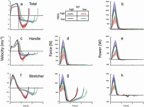
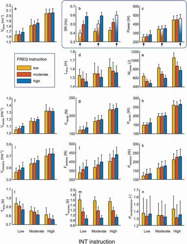
Figure 2. Mean and SD (n = 12) of selected variables against FREQ (colour signature) and INT (x-axis) task instructions. For SR (b) and power (c), the preferred instructions are highlighted by arrows.

While many variables showed large effects for INT and/or FREQ, others were quite small, yet consistent and thereby showing low p-values. The results indicate the following:

When reducing SR (at a given INT instruction), the required power is obtained by higher peak power (p < 0.001 η² = 0.857) and peak force (p < 0.001 handle: η² = 0.905, stretcher: η² = 0.910), a marginal reduction in mean V_drive, a clear but small increase in T_drive, and a moderately but very consistently changed L_drive (Figure 2(a,d) and Table 1). Interestingly, while peak force is considerably increased with reduced SR (Figure 1), mean handle force is marginally and stretcher force more so reduced (p < 0.001 handle: η² = 0.601, stretcher: η² = 0.817). The required (low) SR is primarily obtained by a longer T_recovery compared to the high SR (Table 1).

Table 1. Statistical outcome (p and η²) of the repeated measures GLM including all instructions (two-way 3x3) and preferred conditions only (one-way 1x3).

	p (η^2)
Variable	All instructions		SRpref
	FREQ	INT
Ldrive	<0.001 (0.619)	<0.001 (0.793)	<0.001 (0.688)
Tdrive	<0.001 (0.634)	<0.001 (0.931)	<0.001 (0.973)
Trecovery	<0.001 (0.976)	0.499 (0.061)	<0.001 (0.952)
Trecovery/Tdrive	<0.001 (0.970)	<0.001 (0.865)	<0.001 (0.901)
Vdrive	0.073 (0.212)	<0.001 (0.896)	<0.001 (0.987)
Work per stroke	<0.001 (0.942)	<0.001 (0.988)	<0.001 (0.882)

Reducing power (at a given FREQ instruction) is obtained by a small but very systematic reduction of L_drive (Figure 2(d) and Table 1), a considerable reduction in peak—and mean force (p < 0.001 η² = 0.991), as well as V_drive, and a distinct yet not large increase in T_drive, combined with a hardly affected T_recovery, all leading to an (obvious) reduction of the work per stroke (Figure 2 and Table 1).

FREQ instruction modestly affected the ratio of power delivered at the handle and stretcher (p = 0.019 η² = 0.302), while power instruction had no effect (p = 0.401 η² = 0.080). Relative joint power contributions (Figure 3) were, except for the shoulder, all influenced by both instruction factors (p ≤ 0.001; 0.752≤η² ≥0.598; Table 2). At the shoulder, FREQ instruction had a modest effect.

Figure 3. Mean and SD (n = 12) of relative joint powers against FREQ (colour signature) and INT (x-axis) task instructions. Note that, for between joint comparison reasons, the same scale is used for all joints.

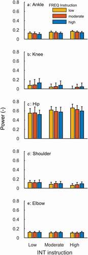
Table 2. Statistical outcome (p and η²) of the repeated measures ANOVA for relative joint powers including all instructions (two-way 3x3) and preferred conditions only (one-way 1x3).

Joint	p (η^2)
	All instructions		SRpref
	FREQ	INT
Ankle	<0.001 (0.752)	<0.001 (0.680)	0.264 (0.114)
Knee	<0.001 (0.598)	<0.001 (0.665)	0.011 (0.336)
Hip	<0.001 (0.647)	<0.001 (0.616)	<0.001 (0.546)
Shoulder	0.023 (0.290)	0.247 (0.119)	0.707 (0.031)
Elbow	<0.001 (0.700)	<0.001 (0.709)	0.019 (0.304)

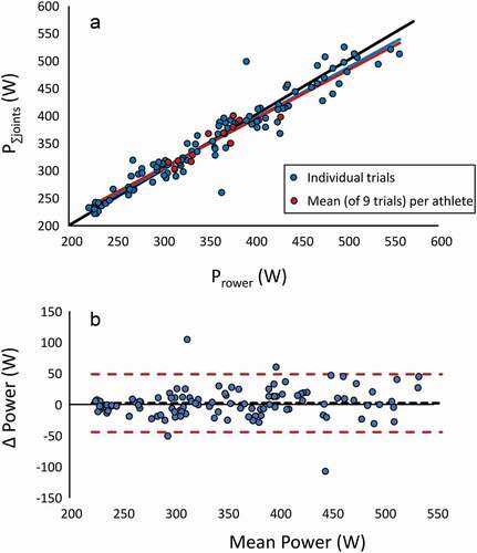
The intrinsic validity check revealed strong similarities between P_∑joints and P_rower, both in the time profile (Figure A1) and regarding mean (paired t-test on mean outcome over all conditions: p > 0.675). The grand total mean of powers between P_∑joints and P_rower differed 2 W, the 95% confidence interval of the difference between calculations amounted to ± 46 W (Figure A2). A strong correlation (r = 0.962 and 0.9) over all and mean data, respectively, as well as the outcome regressed close to the line of identity, with a regression slope of 0.99 (95% C.I. 0.978–1.003) (Figure A2).

Preferred stroke rate instructions

Having established the major effects of FREQ and INT, a comparison of main interest (i.e., how differences between the three intensities executed at preferred SR, SR_pref, compared with overall condition effects) was analysed in more detail comparing the one-way ANOVA with the main 2-way ANOVA. For this purpose, we do not report variables that must have been affected by rule by the combination of altered power and SR (e.g., SR and power itself, absolute force).

General kinetics

The outcome on general kinetics (Table 1) do not confirm our hypothesis that of the nine conditions the three SR_pref conditions would be most alike; all variables analysed still show small p-values and similar large effect sizes for these SR_pref conditions (1-way ANOVA) compared to the 2-way ANOVA (all conditions). This also applies to those variables that theoretically could be independent of these INT-FREQ combinations (e.g., relative drive—and recovery time, L_drive, W_stroke). Even though L_drive and W_stroke seem to show very similar values in the three SR_pref conditions with respect to the variation among all nine conditions Figure 2(d,e), the statistical outcome of 3x3 - and 1-way ANOVAs (Table 1) does not support such notion. For the SR_pref condition, W_stroke (moderate INT 90% and low INT 83% of high INT) is clearly affected by INT instruction, yet far less than SR (84% and 66%, respectively; also see Figure 2).

Joint contributions

For the entire data set (all instruction combinations), INT and FREQ instructions had substantial effects on relative contributions for all joints but the shoulder (Table 2). Yet, for all the joints the absolute differences were very modest (Figure 3). For the preferred SR instructions, the clear effects were indicated for hip only (borderline for the knee and elbow) (Table 2).

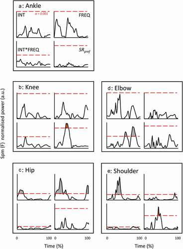
To investigate any effect of protocol on timing of events, time traces of instantaneous power were normalised for amplitude and time for drive only (any deviation in time due to relative drive time and any amplitude difference was established in the first analysis on mean outcome per stroke). These normalised traces for P_rower, P_handle and P_stretcher (the four outer instruction conditions of the 3x3 matrix only) are shown in Figure 4. Even though the traces show strong similarities, systematic differences (all conditions, 3x3 SPM) are recognisable for certain brief periods (coloured areas above threshold line in Figure 5). Note that we rather focus on the lasting periods with relatively high amplitudes of the SPM {F} trace than on what exactly resides above an arbitrary threshold (here chosen conservatively at p = 0.001). The 3x1 SPM on the SR_pref conditions showed some diminishing of these differences for P_stretcher. For joint powers Figure 6, the disappearance or strong reduction of effects in SR_pref conditions at the shoulder and hip (i.e., the most proximal joints), and elbow can be observed. It should be noted that for ankle and knee, no effects were found in the original 3x3 SPM. At the knee, a short-lasting period with noteworthy differences in the SR_pref conditions surfaced.

Figure 4. Mean (n = 12) normalised time traces for total (a), stretcher (b), and handle (c) power for the drive period of the four most extreme combinations of power and stroke rate. Shaded areas are SD.

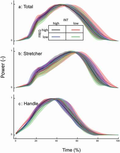
Figure 5. SPM {F} outcome for normalised time profiles of total (a), stretcher (b), and handle power (c) for the full (3x3) condition matrix and SR_pref (1x3) conditions. For each variable, as indicated in Fig. A, three sub-diagrams are from the 3x3 matrix outcome (INT, FREQ and INT*FREQ), the fourth is from the SR_pref conditions. Same set-up in Figs B and C. Alpha threshold is presented by red dashed horizontal line and set at 0.001 (indicated in Fig. A) to isolate the clearest effects from smaller ones. The shaded areas indicate period with effects beyond the threshold.

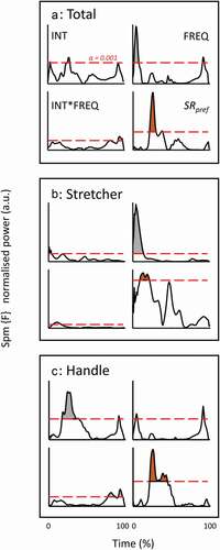
Figure 6. SPM {F} outcome for normalised time profiles of joint powers for the full (3x3) condition matrix and SR_pref (1x3) conditions. For each variable, as indicated in Fig. A, three sub-diagrams are from the 3x3 matrix outcome (INT, FREQ and INT*FREQ), the fourth is from the SR_pref conditions. Same set-up in Figs B to E. Alpha threshold is presented by red dashed horizontal line and set at 0.001 (indicated in Fig. A) to isolate the clearest effects from smaller ones. The shaded areas indicate period with effects beyond the threshold.

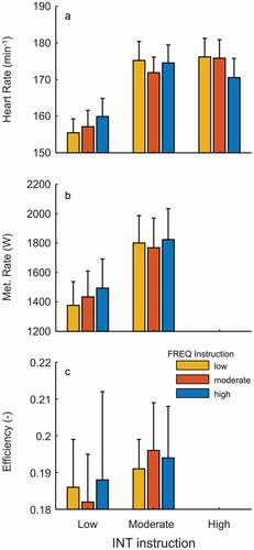
The physiological response is shown in Figure 7. Metabolic rate was strongly affected by both INT (p < 0.001 η² = 0.976) and FREQ (p < 0.001 η² = 0.611). The FREQ effect on metabolic rate was basically nullified when corrected for factual external power differences, that is, expressed as gross efficiency (p = 0.189 η² = 0.14), the INT effect was reduced but still present (p = 0.008 η² = 0.491). INT influenced heart rate (p < 0.001 η² = 0.962), but the difference occurred only between low versus the two other (highest) intensities (post hoc Bonferroni). Heart rate was always lowest at the preferred SR (p < 0.001 η² = 0.649), the other two SRs did not differ meaningfully from each other (post hoc Bonferroni: p = 1 Cohen’s d = 0.122 see also Figure 7). In contrast to metabolic rate, when heart rate was normalised for power (BPM/Watt)—in the same way like when determining efficiency from metabolic rate, that is, dividing the value by power—the effect was only marginally reduced (p = 0.009 η² = 0.352).

Figure 7. Mean and SD (n = 12) of heart rate (a), metabolic rate (b) and efficiency (c) against FREQ (colour signature) and INT (x-axis) task instructions.

Discussion and implications

The purpose of the present study was to examine effects of intensity and stroke frequency on the (relative) kinetics of sliding ergometer rowing in highly trained rowers, including if any of such potential effects counteracted each other at different intensities at preferred SR, resulting in highly similar kinetics for these conditions with preferred SR. The main finding was that SR was mostly regulated by adapting recovery time, leaving the drive kinetics less (but still systematically) affected by FREQ, and more so by power (INT) instruction. The drive was affected by INT and FREQ instruction in a way that allowed the athlete to conform to these protocol instructions: given an instructed SR and thus number of drive actions allowed per minute, the force and power amplitudes during the drive were modified, also depicted in combined but lesser effects on L_drive, T_drive, and V_drive by FREQ instruction (Figures 1 and 2).

Most athletes appeared not readily able to adhere to the instructions perfectly, that is, the power at a given INT instruction (100, 75, and 55% of P_high) was affected by required SR and vice versa. This confirms findings by Hofmijster et al. (2009) in which rowers performed at increasing power when increasing SR despite the instruction to perform at the same power. Thus, the details that are discussed here should be considered within a framework of what the athlete is able to do rather than the outcome of the “virtual” athlete who is perfectly executing the tasks by instruction. It must be noted that it is too simple to consider the kinematic variables as mere outcome muscle dynamics; the kinematics reciprocally affect muscle dynamics. The entanglement of dependencies and mechanisms, given the stringent constraints induced by the ergometer properties, likely leads to a tight natural coupling of power and SR. Therefore, it is likely that the athlete is strongly challenged when asked to produce a given power at another than the preferred SR.

The current findings support the notion that in ergometer rowing, as well as on-water rowing, intensity is mostly regulated through SR (Holsgaard-Larsen & Jensen, 2010), yet the mechanism is fairly complicated. First, the evidence for this notion itself is found in the strongest effect of FREQ instruction on T_recovery compared to T_drive. Yet, T_drive is clearly affected as well, which must be regarded in the light of the physical constraints imposed in rowing. The relatively small effects of INT instruction (as well as FREQ) on the velocity of motion (Figure 1) may be explained by the viscous nature of air (ergometer rowing) and water (on-water rowing) resistance: a more intense drive (i.e., faster generation of higher forces) results in moderate drive velocity increases because velocity exponentially dictates the required force. In other words, generating more handle force results in higher power, but only a moderate increase in speed of the athlete’s motion. Thus, the effect on T_drive is restrained by the nature of resistance (also see Hofmijster et al., 2009), and the required increase in SR to deliver the desired power (given the W_stroke) is obtained by adjusting T_recovery. We hypothesise that even though power is regulated through SR, this is only done so indirectly: first, W_stroke is ‘set’ for the power requirement (leading to a given T_drive), but an additional SR adjustment is needed which is done by T_recovery modification. Interestingly, this mechanism does not seem to be dictated by constraints regarding W_stroke, that is, both lower and higher W_stroke were obtained during various of other than SR_pref conditions. How this principle transfers to on-water rowing is beyond the scope of the current study. Yet, one may suggest that a higher oar force and water resistance reduces the oar motion relative to the water, thus increasing propulsion efficiency. As in ergometer rowing, the higher oar force should then lead to a faster movement of the boat over water, with only some increase in athlete’s drive movement speed. Thus, while power can be regulated through applied force that moderately affects the drive movement speed and time, the targeted power is finally obtained by modifying recovery time accordingly.

L_drive was not set by instruction nor dictated by the ergometer. Although the athletes did modify L_drive, the decrease in L_drive with higher SR (at a given power) was not dramatic, and L_drive was mostly affected (increased) by power instruction (largest difference 8%) (Figure 2(d)). This rather small change in L_drive is similar to what has been shown (Hofmijster et al., 2007). In general, rowers maintain their L_drive and work per stroke quite constant across a range of intensities (power outputs), both in on-water and ergometer rowing. This is likely due to the ‘dynamics of increased resistance’ when force is increased (water, air, see above), as well as the likely benefit of keeping drive and muscle contraction dynamics (mainly length and velocity) as constant as possible during different rowing intensities. Thus, an increase in power output is mainly done by an increase in SR (and opposite to, e.g., running, in which mostly stride length is increased, at least at low to moderate speeds (Schache et al., 2014)). The guiding role of L_drive, even if it is moderately affected, is highlighted by its enhanced effect size for the SR_pref conditions (Table 1). Overall, an increase in SR (at a given P_mean) leads to a decrease in T_drive and L_drive, thereby V_drive is kept approximately constant at a given power. Obviously and as mentioned earlier, all these variables are mechanically interlinked, and it is not possible to directly deduce any simple cause–effect relationship between these variables from this analysis.

The shape of the time profiles for power and speed (as well as force, not shown) (Figures 1 and 4) are very similar, independent of instruction. This opts for the rationale that the constraints imposed on the task by the rowing ergometer, instruction, and athlete makes the athlete execute the task in a stereotyped manner. Even so, many details of the outcome, for example, timing of events and relative amplitude of such events, clearly seem affected by instruction. We hypothesised that the three natural SR_pref conditions would show the closest kinetic resemblance among all nine conditions. The general outcome of the comparison of the statistical analysis (Table 1) did not clearly support this notion. Compared to all nine conditions, among the SR_pref conditions, the instruction effect on L_drive seems enhanced, the dependence of T_recovery on FREQ instruction is not diminished, the same applies to the dependence of T_drive and V_drive on INT instruction. Still, the regulation of intensity by SR leads to a reduced effect on work per stroke in the SR_pref conditions (Table 1). This is also shown in Figure 1(b,e,h): the SR_pref conditions show power profiles that are closest neighbours. Thus, the strong role of SR in intensity steering seemingly keeps the required variation of work per stroke and instantaneous power within limits in both directions. The differences in the kinematics may be regarded a way to accomplish this and, in that case, to be regarded as a sign of versatility of the movement system.

The analysis at the joint level (Table 2) confirmed our hypothesis in part. The instruction effects on hip relative contribution in power were not smaller among the SR_pref conditions compared to effects for all nine instruction conditions, but at the other joints this was the case. It should be noted that the hip was the main joint at which power generation occurred. The low contribution at the knee can be explained by a period of negative power (see also Greene et al. (2013), that is, an apparent power absorption, which most likely is depicting power generated by knee extensors (vasti) but transferred to the hip via biarticular hamstrings, as in cycling (Gregor et al., 1985; Martin & Nichols, 2018; van Ingen Schenau et al., 1992). Interestingly, the time profiles of normalised joint power showed an almost opposite outcome (Figure 6). The ankle and knee showed no effects in any way, while the instruction effects for hip joint did not show in the SR_pref conditions. Only at the knee, a small instruction effect emerged in SR_pref. The latter is hard to explain. Still, at the coordinative (joint) level, the overall impression is that these time profiles show highest similarity of power generation features in the SR_pref conditions compared to the others. Yet, this did not apply for external power (Figures 4 and 5). One may speculate that this disagreement may be due to the strict constraints of the task, that is, a limited number of possible ways in which segmental (and joint) rotations can be best transferred into handle and stretcher translation. If one takes the departure point that these athletes are well capable to execute a coordination pattern leading to high metabolic efficiency and efficacy (Bobbert & van Soest, 2001), the shape of the external power profile may not be the key parameter to study, but rather the coordinative joint profile that are an expression of effective (i.e., good efficiency and efficacy) muscle activity.

With respect to the physiological response and metabolic cost our present results confirm the findings by Hofmijster et al. (2009), that is, energetic optimisation hardly seems to play a role of importance for the choice of SR_pref. Even though metabolic rate was clearly affected by FREQ, this effect is explained by the small differences in actual external power delivered during the exercises. That is, gross efficiency is almost independent of FREQ, the differences marginal in size. The INT effect is fully explained by the power difference between low and moderate intensity as explained in Ettema and Lorås (2009). In accordance with Hofmijster et al. (2009) and Holt et al. (2021) our findings open for the possibility that rowers choose a stroke rate that maximises boat speed for a given power delivery, not energetic efficiency. Still, our heart rate findings suggest that some aspects of physiological load may be reduced at the preferred SR. This notion is however no incitement for using HR as measure for physiological stress; the validity assessment of HR for purpose is beyond the scope of the current study.

Methodological consideration

Few studies are found on full inverse dynamics that allows the analysis of joint power profiles. To our knowledge, only one other group seems to have performed a more in-depth analysis (Attenborough et al., 2012; Greene et al., 2009, 2013) Our approach was like theirs, be it with some essential differences. It is beyond the scope of this paper to discuss the consequences of these differences, yet a profound comparison of the power time profiles, and relative joint contributions may give an indication of the validity of our and their (Attenborough et al., 2012; Greene et al., 2009) approaches and findings. The intrinsic validity check (by comparing external power with the sum of joints power) on our own data are promising; the total power as well as details of the time profiles show minimal differences, which implies no or little unaccounted power in trunk motion or in other planes not incorporated in the inverse dynamics analysis. Still, how much of such trunk power is allocated to either shoulder or hip cannot be elucidated. For the current purpose of study, that is, investigating effects of FREQ and INT, our approach seems satisfactory.

Summarising conclusion

Our results show that ergometer rowing at different intensities and stroke rates show very similar technical time profiles at the level of external and joint power. Rowers adjust details of these profiles to adhere to the instructions as well as possible. It seems that rowing at preferred SRs (which depends on and regulates power) is technically very similar, while differences increase when obliged to apply other SRs. Thus, rowing at lower intensities may be highly relevant for high intensities regarding technique.

Acknowledgement

We thank the participants and Johan Flodin for their involvement and time.

Disclosure statement

No potential conflict of interest was reported by the author(s).

Additional information

Funding

The author(s) reported there is no funding associated with the work featured in this article.

Appendix

The validity of the approach for the inverse dynamics (details described in main text) was examined by comparing the total external power, that is, sum of stretcher, handle, and rate of change of body mass energy (e.g., Danielsen et al., 2019) with the power obtained from summing joint powers. These ways of obtaining total power delivered by muscles are identical in theory. Thus, comparing these, both on mean and time profile, provides a justification of the inverse dynamics approach (as well as sufficient accuracy of measurement). Any strong deviation indicates flaws in either model, strong similarities do not prove validity but make the occurrence of serious flaws unlikely. This assessment does not examine the consequences of the simplifications of the model: Modelling of a stiff trunk between shoulder and hip may have associated some of power produced within the (flexible) trunk to the hip or shoulder, but mostly ignores such power. This matter cannot be elucidated by the present validation. On a general note, any such simplification that generally is made in inverse dynamics modelling is difficult to validate. Figures A1 and A2 show the outcome of the comparison, which is briefly discussed in the main text.

Figure A1. (a) Mean (n=12) time traces for P_rower (red) and P_∑joints (black). Shaded areas are SD. Sub-diagrams show results for the instruction combinations of FREQ (column-wise) and INT (row-wise). Combinations of stroke rate and power are indicated. (b) The corresponding SPM {t} outcome for the trace differences. Alpha threshold is presented by red dashed horizontal line and set at 0.001 (indicated in top-left diagram).

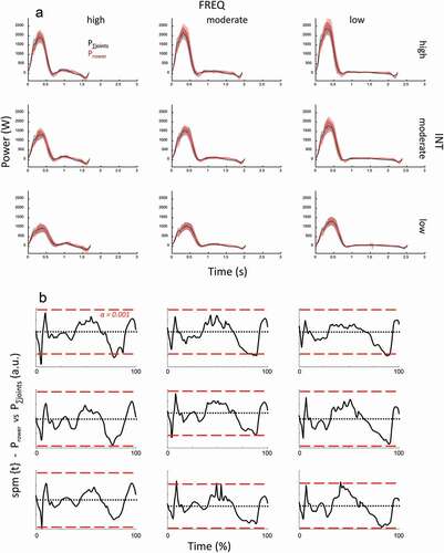
Figure A2. (a) Correlation analysis of P_rower and P_∑joints. Regression lines (colour signature) for all individual trials and mean (of 9 trials) for each athlete, as well as line of identity (black) are indicated. (b) Bland-Altman diagram of the same data.

References

- Attenborough, A. S., Smith, R. M., & Sinclair, P. J. (2012). Effect of gender and stroke rate on joint power characteristics of the upper extremity during simulated rowing. Journal of Sports Sciences, 30(5), 449–458. https://doi.org/10.1080/02640414.2011.616949
- Bobbert, M. F., & van Soest, A. J. (2001). Why do people jump the way they do? Exercise and Sport Sciences Reviews, 29(3), 95–102. https://doi.org/10.1097/00003677-200107000-00002
- Danielsen, J., Sandbakk, O., McGhie, D., & Ettema, G. (2019). Mechanical energetics and dynamics of uphill double-poling on roller-skis at different incline-speed combinations. Plos One, 14(2), e0212500. https://doi.org/10.1371/journal.pone.0212500
- de Leva, P. (1996). Adjustments to Zatsiorsky-Seluyanov’s segment inertia parameters. Journal of Biomechanics, 29(9), 1223–1230. https://doi.org/10.1016/0021-9290(95)00178-6
- Elftman, H. (1939). Forces and energy changes in the leg during walking. The American Journal of Physiology, 125(2), 339–356. https://doi.org/10.1152/ajplegacy.1939.125.2.339
- Elliott, B., Lyttle, A., & Birkett, O. (2002). Rowing. Sports Biomechanics, 1(2), 123–134. https://doi.org/10.1080/14763140208522791
- Ettema, G., & Lorås, H. W. (2009). Efficiency in cycling: A review. European Journal of Applied Physiology, 106(1), 1–14. https://doi.org/10.1007/s00421-009-1008-7
- Gorman, A. J., Willmott, A. P., & Mullineaux, D. R. (2021). The effects of concurrent biomechanical biofeedback on rowing performance at different stroke rates. Journal of Sports Sciences, 39(23), 2716–2726. https://doi.org/10.1080/02640414.2021.1954349
- Greene, A. J., Sinclair, P. J., Dickson, M. H., Colloud, F., & Smith, R. M. (2009). Relative shank to thigh length is associated with different mechanisms of power production during elite male ergometer rowing. Sports Biomechanics, 8(4), 302–317. https://doi.org/10.1080/14763140903414391
- Greene, A. J., Sinclair, P. J., Dickson, M. H., Colloud, F., & Smith, R. M. (2013). The effect of ergometer design on rowing stroke mechanics. Scandinavian Journal of Medicine & Science in Sports, 23(4), 468–477. https://doi.org/10.1111/j.1600-0838.2011.01404.x
- Gregor, R. J., Cavanagh, P. R., & LaFortune, M. (1985). Knee flexor moments during propulsion in cycling—A creative solution to Lombard’s Paradox. Journal of Biomechanics, 18(5), 307–316. https://doi.org/10.1016/0021-9290(85)90286-6
- Held, S., Siebert, T., & Donath, L. (2020). Changes in mechanical power output in rowing by varying stroke rate and gearing. European Journal of Sport Science, 20(3), 357–365. https://doi.org/10.1080/17461391.2019.1628308
- Hofmijster, M. J., Landman, E. H., Smith, R. M., & Van Soest, K. (2007). Effect of stroke rate on the distribution of net mechanical power in rowing. Journal of Sports Sciences, 25(4), 403–411. https://doi.org/10.1080/02640410600718046
- Hofmijster, M. J., Van Soest, A. J., & De Koning, J. J. (2008). Rowing skill affects power loss on a modified rowing ergometer. Medicine and Science in Sports and Exercise, 40(6), 1101–1110. https://doi.org/10.1249/MSS.0b013e3181668671
- Hofmijster, M. J., Van Soest, A. J., & De Koning, J. J. (2009). Gross efficiency during rowing is not affected by stroke rate. Medicine and Science in Sports and Exercise, 41(5), 1088–1095. https://doi.org/10.1249/MSS.0b013e3181912272
- Holsgaard Larsen, A., & Jensen, K. (2010). Ergometer rowing with and without slides. International Journal of Sports Medicine, 31(12), 870–874. https://doi.org/10.1055/s-0030-1265148
- Holt, A. C., Ball, K., Siegel, R., Hopkins, W. G., & Aughey, R. J. (2021). Relationships between measures of boat acceleration and performance in rowing, with and without controlling for stroke rate and power output. Plos One, 16(8), e0249122. https://doi.org/10.1371/journal.pone.0249122
- Ingham, S. A., Whyte, G. P., Jones, K., & Nevill, A. M. (2002). Determinants of 2,000 m rowing ergometer performance in elite rowers. European Journal of Applied Physiology, 88(3), 243–246. https://doi.org/10.1007/s00421-002-0699-9
- Martin, J. C., & Nichols, J. A. (2018). Simulated work loops predict maximal human cycling power. The Journal of Experimental Biology, 221, 13. https://doi.org/10.1242/jeb.180109
- McShane, B. B., Gal, D., Gelman, A., Robert, C., & Tackett, J. L. (2019). Abandon Statistical Significance. The American Statistician, 73(sup1), 235–245. https://doi.org/10.1080/00031305.2018.1527253
- Pataky, T. C., Robinson, M. A., & Vanrenterghem, J. (2013). Vector field statistical analysis of kinematic and force trajectories. Journal of Biomechanics, 46(14), 2394–2401. https://doi.org/10.1016/j.jbiomech.2013.07.031
- Peronnet, F., & Massicotte, D. (1991). Table of nonprotein respiratory quotient: An update. Canadian Journal Sport Science, 16(1), 23–29.
- Schache, A. G., Dorn, T. W., Williams, G. P., Brown, N. A. T., & Pandy, M. G. (2014). Lower-limb muscular strategies for increasing running speed. The Journal of Orthopaedic and Sports Physical Therapy, 44(10), 813–824. https://doi.org/10.2519/jospt.2014.5433
- Tomiak, T., Gorkovenko, A. V., Mishchenko, V. S., Korol, A., Bulinski, P., Vereschaka, I. V., Tal’nov, A. N., & Vasilenko, D. A. (2016). Control of the power of strokes and muscle activities in cyclic rowing movements (a research using rowing simulators). Neurophysiology, 48(4), 297–311. https://doi.org/10.1007/s11062-016-9602-x
- van Ingen Schenau, G. J., Boots, P. J., de Groot, G., Snackers, R. J., & van Woensel, W. W. (1992). The constrained control of force and position in multi-joint movements. Neuroscience, 46(1), 197–207. https://doi.org/10.1016/0306-4522(92)90019-X
- van Ingen Schenau, G. J., & Cavanagh, P. R. (1990). Power equations in endurance sports. Journal of Biomechanics, 23(9), 865–881. https://doi.org/10.1016/0021-9290(90)90352-4