Bridging the lab-to-field gap using machine learning: a narrative review

ABSTRACT

This paper summarises recent advancement in applications of machine learning in sports biomechanics to bridge the lab-to-field gap as presented in the Hans Gros Emerging Researcher Award lecture at the annual conference of the International Society of Biomechanics in Sports 2022. One major challenge in machine learning applications is the need for large, high-quality datasets. Currently, most datasets, which contain kinematic and kinetic information, were collected using traditional laboratory-based motion capture despite wearable inertial sensors or standard video cameras being the hardware capable of on-field analysis. For both technologies, no high-quality large-scale databases exist. A second challenge is the lack of guidelines on how to use machine learning in biomechanics, where mostly small datasets collected on a particular population are available. This paper will summarise methods to re-purpose motion capture data for machine learning applications towards on-field motion analysis and give an overview of current applications in an attempt to derive guidelines on the most appropriate algorithm to use, an appropriate dataset size, suitable input data to estimate motion kinematics or kinetics, and how much variability should be in the dataset. This information will allow research to progress towards bridging the lab-to-field gap.

KEYWORDS:

• Machine learning
• artificial neural networks
• motion analysis
• inertial sensors
• video analysis

Introduction

During the last decades, machine learning (ML) has become more prominent in our daily lives, either as part of recommendation systems (e.g., Netflix (Steck et al., 2021) or Amazon (Belacel et al., 2020)), or in fitness trackers (e.g., Fitbit (Haghayegh et al., 2020) or Garmin (G. Ltd., 2023)). A similar uptake of ML can be found in the scientific literature, spanning a variety of research fields (Xu et al., 2021), including sports biomechanics. Many applications of ML in sports biomechanics involve the development of tools for on-field motion analysis (Dindorf et al., 2023). In this paper, I will summarise recent advancement in this area as presented in the Hans Gros Emerging Researcher Award lecture at the annual conference of the International Society of Biomechanics in Sports 2022.

One major problem of data-driven approaches (such as ML) is that they are optimised for the data they have been trained on. This is particularly a problem when ML is used for small datasets: the ML model cannot generalise to new data (Goodfellow et al., 1997). This lack of generalisability can be prevented by using large training datasets with high variance. For example, commonly used datasets for image classification tasks in medicine are PatchCamelyon (Veeling et al., 2018) that consists of 327,680 images extracted from histopathological lymph node scans or ChestX-ray8 (Wang et al., 2017) that contains 108,948 frontal-view X-ray images of 32,717 unique patients. Datasets at this scale can hardly, if ever, be found in sports biomechanics.

For the last decades, motion analysis mainly took place inside specialised laboratories using optical motion capture setups. These setups are expensive, time-consuming to use, and cannot be used for on-field analysis because of their restriction to space and lighting conditions. However, many high-quality but small-scale datasets are available. Recently, inertial sensors and two-dimensional videos have become increasingly popular for on-field motion analysis, but large high-quality datasets using these technologies containing kinematic and kinetic information are missing. Therefore, methods to artificially enlarge inertial sensor and video datasets leveraging existing optical motion capture datasets need to be developed and applied. The second major issue in ML in sports biomechanics is the missing availability of guidelines for the design and use of ML in the area. This article provides a brief introduction to machine learning (Section 2), summarises methods that re-purpose motion capture data to synthesise inertial sensor or video data (Section 3), and aims to provide guidelines on the use of ML for motion analysis (Section 4).

A brief introduction to machine learning

ML can be defined as: ‘A computer program is said to learn from experience E with respect to some class of tasks T and performance measure P, if its performance at tasks in T, as measured by P, improves with experience E’. (Mitchell, 1997). In general, ML algorithms provide statistical solutions if a deterministic solution is difficult to implement or time-consuming to execute. Different tasks T that can be solved using ML algorithms are classification, clustering, or regression. In contrast to classification or clustering, where the ML algorithm learns to distinguish between groups of data, in regression tasks the algorithm needs to estimate a numerical value as output. The performance measure P is used to evaluate the accuracy of the estimated values compared to the target. P needs to be defined specifically for each task T and should improve with each experience E (Goodfellow et al., 1997).

The most commonly used ML algorithm in sports biomechanics is Artificial Neural Networks (ANNs). ANNs fundamentally are universal function approximators (Cybenko, 1989). Instead of explicitly programming the solution of one specific task, they learn the optimal solution from existing data. ANNs were inspired by the structure of the human brain, consisting of multiple neurons arranged in layers that represent the capacity of the network. There are multiple classes of ANNs, varying in complexity, due to the large range of tasks which they are suited to and typically used for (Goodfellow et al., 1997).

Multilayer perceptron (MLP) networks are the earliest and simplest class of ANNs. They consist of neurons (a mathematical operation) that are arranged in multiple layers. Besides the input and output layers, they can have a varying number of hidden layers. While the input and output layer solely contain the initial data and result for the given input data, the hidden layers are layers of mathematical functions, each designed to produce an output specific to the intended result. Each neuron in one layer is connected to all neurons in the previous and subsequent layer. An ANN with a single hidden layer consisting of a sufficient number of neurons can approximate any continuous function to any desired precision (Cybenko, 1989). MLP networks are flexible and are used to learn relationships between inputs and outputs for classification or regression tasks. By flattening image or time series data, MLP networks can be used to process time-sequence input data. However, the flattening removes the time dependency of the data and increases the number of inputs which makes it more difficult to find the time-dependent patterns that are most relevant to sequential data. Although MLP networks are easy to train, they are limited to time-normalised data and are computationally expensive. Consequently, MLP networks provide baseline information for the predictability of all types of data and make them a good starting point (Goodfellow et al., 1997).

As an alternative, recurrent neural networks (RNNs) were developed specifically for natural language processing. RNNs can learn time-dependent patterns from sequences of arbitrary lengths as a result. They process only the preceding time steps and not the complete sequence. In contrast to MLP networks, they have time-delayed inner recursions and inner states that serve as a memory. Unfortunately, RNNs suffer from compounding errors during training. To overcome this problem, long short-term memory (LSTM) neural networks were introduced. The difference between an LSTM network and a standard RNN are the LSTM network’s gate layers, that ensure that only the most relevant time-dependent relationships are maintained. While classic LSTM networks can only learn future time dependencies, bidirectional LSTM networks have been adopted recently. In these networks the sequence information can flow in both directions: backwards (future to past) or forward (past to future). The major downside of LSTM networks is that they are intensive to train and require large datasets (Goodfellow et al., 1997).

The third most common class of ANNs, known as a Convolutional Neural Network (CNN), was originally designed for the classification task of mapping image data to a single output variable. CNNs learn from raw image data by exploiting correlations between local pixels, hence they are particularly suited for modelling spatial relationships. Ordered relationships are also inherent in time series data, which makes CNNs suited for time series estimation. Due to the popularity of image classification tasks in the computer science domain, many open-access models have been developed and trained using large quantities of data. These models can either be re-trained from scratch or fine-tuned with task-specific data. Fine-tuning has the advantage that the model can leverage previous training processes. On the downside, inputs need to be similar to the original training data, which increases the pre-processing steps required prior to implementation (Goodfellow et al., 1997).

One major problem of data-driven approaches is that they are optimised for the data they have been trained on. This is particularly a problem when ML is used for small datasets. If the capacity of a ML model is too large and the dataset is too small, the model is only suitable for the specific patterns within the training data and cannot find patterns in new data; it overfits its training data. If the capacity of the model is too low, it cannot represent the relevant features in the training data; it underfits its training data. To avoid underfitting, the capacity of the model needs to be enlarged using more neurons or layers, which increases the likelihood of overfitting. To prevent a model from overfitting, different regularisation strategies have been proposed. The simplest regularisation strategy to prevent the model from overfitting is early stopping of the training procedure. A more sophisticated, regularly employed regularisation strategy is dropout. Dropout means that individual neurons of a network are randomly switched off during the training process to prevent these neurons from specialising in specific features (Goodfellow et al., 1997).

Overfitting can further be prevented by using large training datasets with high variance, that currently can only be found for optical motion capture in sports biomechanics, but not for inertial sensor or video data. Optical motion capture has been the state-of-the-art method for decades and usually includes both the collection of kinematic and kinetic information. Similarly, video cameras have been used for decades, but only to analyse kinematics, while inertial sensors just recently provided sufficient accuracy to be used in motion analysis and only for the determination of kinematic parameters. Therefore, no large datasets containing both kinematics and kinetics exist. To circumvent this problem, historical optical motion capture data can be re-purposed.

Re-purposing 3D optical motion capture data

Applications in sports biomechanics that aim for high-fidelity motion analysis rely on datasets that are collected by traditional optical motion capture setups. These setups allow for highly accurate determination of motion parameters, but are expensive, time-consuming to use, need expert knowledge, and a specific laboratory environment. Therefore, many high-quality datasets exist, but usually comprise a small number of participants. By combining multiple of these small, historical datasets, larger datasets with high variance can be created. However, this setup cannot be used for on-field analysis because of its restriction to a laboratory environment. Hence, investigations using motion capture data for machine learning applications are not fit for purpose of on-field analysis. They are promising first steps, but still a fair way off bridging the gap to the field.

Wearable sensors and video cameras are sought to provide the hardware for the next step towards the accurate measurement of biomechanical variables on-field. Inertial sensor systems consisting of accelerometers, gyroscopes, and magnetometers can be used to determine 3D motion kinematics, but do not provide information about kinetics and restrain an athlete’s movement. Capturing movement with video cameras does not inhibit the athlete but is generally restricted to 2D or pseudo-3D kinematics and—similar to inertial sensors—does not provide kinetic information. To provide the missing information on 3D motion kinematics and kinetics, machine learning tools are developed; oftentimes using small datasets of less than 30 participants, e.g., (Aljaaf et al., 2016; Argent et al., 2019; Camargo et al., 2022; Dorschky et al., 2020; Renani et al., 2021).

The limited availability of large wearable sensors’ datasets causes the missing link between laboratory and on-field applications. There are large datasets of gold-standard optical motion capture in conjunction with force plate data, but only very small datasets containing kinematic information collected with inertial sensors or video cameras and accompanying kinetic data from force plates. For this reason, there is a need to develop methods to create larger synthesised datasets that contain inertial sensor (Section 3.1) or video data (Section 3.2) and kinetic information to be able to make sensible use of ML methods and create generalised models for on-field analysis. This can be achieved by re-purposing historical motion capture data.

Inertial sensor data

The first attempt to synthesise inertial sensor data (acceleration, angular rate, and magnetic field strength) from optical motion capture data was made by Young et al. (2011). Their complex framework could model sensor noise, bias, misalignment, cross-axis effects, and field distortions as well as more general sensor network issues such as time synchronisation and packet losses in the synthesised data. This work offers a great simulation toolbox, but the validation was carried out with a single participant walking, which raises questions about its broader applicability. Furthermore, they attached markers to the inertial sensor to derive position and orientation; information that is not available in historical motion capture datasets.

Brunner et al. (2015) developed a similar workflow designed for synthesising inertial sensor data including magnetic distortion. They used the sensor’s global position and rotation as input to their model and validated the framework using a three-axis table; hence, there is no information on how this framework performs on human movement. Another limitation is that the global position of an inertial sensor is in general not available.

Zimmermann et al. (2018) used a simplified approach to synthesise inertial sensor data to develop an automated deep-learning framework for sensor-to-segment-assignment and sensor-to-segment-alignment. Their work was the first to use synthesised data to enlarge a sparse inertial sensor database for an ML application. They did not provide further details on their simulation framework and validated their results for a single participant and sensor position only.

Building on this previous work, we synthesised segments’ acceleration and angular rate from motion capture data. Our first aim was to demonstrate that synthesised inertial sensor data of seven sensors—pelvis, thighs, shanks, and feet—can be used to estimate joint angles and joint moments using an artificial neural network (ANN) (Mundt, Thomsen, et al., 2019). The subsequent aim was to show that synthesised data can be used to enlarge a sparse measured inertial sensor dataset for the same task (Mundt, Koeppe, David, Witter, et al., 2020). We validated the synthesising approach for five inertial sensors fixed to the pelvis, both thighs and both shanks of 30 participants during walking trials. Since we used optical motion capture data as ground-truth, the walking trials were undertaken in a laboratory environment.

The framework we used was rather simple to allow for fast computation and ease-of-use. The following steps were undertaken to derive synthesised inertial sensor acceleration and angular rate (Mundt, Koeppe, David, Witter, et al., 2020):

1. Calculate segment coordinates systems based on the recommendations of the International Society of Biomechanics (Wu et al., 2002).

2. Transform coordinate systems consisting of x, y, and z-axis to quaternions.

3. Translate and rotate the segment quaternions to initial sensor position and orientation.

4. Calculate the numerical quaternion derivative of the sensor orientation to determine the angular rate.

5. Calculate the linear acceleration of each sensor as the second derivative of the origin of the segment coordinate system and transform those to the local sensor coordinate system considering gravity.

The synthesised data showed very good agreement with the measured data (Figure 1). The best agreement was found for the sensor attached to the pelvis and decreasing agreement for thighs and shanks. These differences can be attributed to the increase in noise due to soft tissue artefacts caused by the impact of the foot with the ground in those sensors attached to segments closer to the ground, that is missing in the synthesised data. The same framework was adopted by Rapp et al. (2021).

Figure 1. Accuracy of synthesised and measured inertial sensor data.

More recently, Dorschky et al. (2020) not only synthesised inertial sensor data from motion capture but also used a biomechanical model and an optimal control problem to simulate new motion trials based on actual trials. The purpose of simulating new trials was to augment an inertial sensor database for machine learning methods. However, the agreement between measured and simulated data was not reported. The computational cost of the proposed method was high (the simulation of a single new trial exceeded 3 min) but resulted in a wider spread of input and output data for the machine learning model.

As a freely available, user extensible software system, OpenSIM offers the opportunity to synthesise inertial sensor data from a marker driven musculoskeletal model (Bicer et al., 2022; Renani et al., 2021). Renani et al. (2021) first enlarged their motion capture dataset of 30 participants by applying magnitude offsets, magnitude warping, combinations of magnitude offsets and warping, time warping, and combinations of time warping and magnitude warping to joint angles to derive synthesised inertial sensor data from these augmented joint angles. The validation of the synthesised inertial sensor data resulted in high accuracy in some sensors and axes (thigh z-axis r = .95, shank x-axis r = .83, y-axis r = .85, z-axis r = .98, foot y-axis r = .98, z-axis r = .85) and lower accuracy in others (pelvis x-axis r = .62, y-axis r = .29, z-axis r = .52, thigh x-axis r = .67, y-axis r = .61, foot x-axis r = .39). Bicer et al. (2022) similarly enlarged their dataset first using generative adversarial networks (GANs) to create new samples and derived synthesised inertial sensor data using OpenSIM. However, the synthesised inertial sensor data was not validated.

Wearable sensors offer a great opportunity for on-field motion analysis. However, these sensors need to be attached to an athlete’s body, which might inhibit their movement or might not be allowed in competition. Therefore, the use of 2D video for high-fidelity motion analysis is even more desirable.

Pose estimation based on video data

The use of computer vision-based pose estimation models to obtain human poses from 2D video data has become increasingly popular in biomechanics because they are easily accessible, do not rely on specific equipment, and allow for quick analysis of video data without manual labour. However, datasets containing 2D video data, optical motion capture data, and force plate data are required to create biomechanically accurate pose estimation models but are incredibly rare. To overcome this limitation, we used animation software (Blender, v.2.79, Blender Foundation, Amsterdam, The Netherlands) to synthesise videos from motion capture trials that have been accompanied by video data. The synchronised datasets allowed us to validate our approach and apply it to other motion capture datasets that never contained video data (Mundt, Goldacre, et al., 2022; Mundt, Oberlack, et al., 2021, 2022).

We developed a seven-step workflow to create synthesised videos from motion capture data. Only two steps could not be automated: the 3D human silhouette needed for the animation had to be created manually and manual adjustment of the motion capture data was required due to a misalignment of the 3D static motion capture trial and 3D silhouette. Since historical motion capture datasets were not collected for the purpose of animation, the static posture adopted by participants and position of the participant in the laboratory’s global coordinate system was not standardised (Mundt, Oberlack, et al., 2022). For future data capture, standardisation of static trials should be considered to simplify animation. To create animations from historical datasets more efficiently, an automated approach to overcome the challenge of missing alignment needs to be developed; potentially using more sophisticated computer vision techniques instead of simple animation workflows. The calculation of joint centres, creation of a static rig, coupling of the rig to the dynamic trial, static morphing of the silhouette, coupling of the silhouette to the dynamic trial, and the creation of different camera views has already been fully automated.

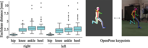
We used OpenPose (Z. Cao et al., 2019), which is a commonly used open-source pose estimation model in biomechanics, to determine 25 anatomically related keypoints and compared the keypoints detected in real and synthesised video data for 47 side stepping trials of three participants. Since we did not use upper limb markers during data collection, the animated silhouette’s arms stayed in a T-pose and keypoints estimated for the upper limbs could not be compared. The overall difference between both real and synthesised videos was smaller than 3.5 mm for the hip, knee, and ankle keypoints. The difference became larger the further the estimated keypoint was away from the origin of the root coordinate system (the centre point between both hips) (Figure 2). Therefore, the increasing difference may be attributed to error propagation. The overall difference was still small, so we accepted the approach as feasible (Mundt, Oberlack, et al., 2021, 2022).

Figure 2. Difference between keypoints estimated in real and synthesised videos. Note that the marker set used during data collection did not contain upper body markers, hence, the arms of the animated silhouette stay in a T-pose and keypoints of the upper limbs cannot be compared.

We applied the developed workflow to a very specific and more complex dataset of elite long jump. The original dataset did not contain any video data to validate the estimated keypoints, but optical verification of the animated videos showed promise (Mundt, Oberlack, et al., 2021, 2022).

We further investigated the possibility to calculate 2D keypoints from 3D motion capture data to allow for a more computationally efficient way to synthesise keypoint data since no videos need to be rendered and no pose estimation needs to be run. This approach would enable us to create near-infinite synthesised trials of keypoints. However, the approach still needs validation by comparison to actual video data (Mundt, Goldacre, et al., 2022).

Synthesising video data is of high interest in computer vision because of the need for large, high-quality datasets. Greff et al (2022) recently suggested a framework to synthesise annotated image and video data based on motion capture data that might enable biomechanists to create training data for ML models at scale. However, the number of effective software solutions to synthesise data is limited and generally task-specific. The use of current open-source pose estimation algorithms for applications that depend on the detection of accurate joint centres is questionable because the models are not able to detect joint centres according to biomechanics standard since they are not trained on a biomechanically informed dataset (Rapczy Nski et al., 2021). This highlights the need for more research in this direction.

Machine learning in sports biomechanics

In the last five years, machine learning (ML) methods have seen a huge adoption in sports biomechanics (Figure 3). This is most likely a result of the increased availability of open-source ML code, which lowers the barrier of entry to make use of this advancing technology.

Figure 3. Machine learning has seen a huge uptake in sports biomechanics in the last five years.

In a systematic review of the literature, we found that many recent publications showed a large gap between what the application promised to achieve and the actual outcome, such as classification of movement quality without clear rational, or injury prevention screening tools that are trained on uninjured athletes. These publications run the risk of being misleading for researchers, sport practitioners, and athletes, and show the need for greater awareness of the potential impact that false promises can have. This is especially important because most publications that over-promise and under-deliver were found in applications that monitor the health of athletes or provide feedback, which have the most potential to cause harm to an athlete’s health, performance, or career.

Applications that provide first steps towards on-field motion analysis tools showed a high agreement between promise and reality. However, most of these applications were still reliant on motion capture data collected in a laboratory in the first instance, which highlights that ML in biomechanics is in its infancy and is not a magic tool. The aim of providing accurate motion information in on-field settings seems to lie further ahead than many research papers suggest. More research is needed to overcome the difficulties of on-field measurement of 3D motion kinematics and kinetics.

Many studies apply ML to very niche populations using small datasets (often less than 20 participants) with small variability and promise a generalised model as outcome. Since ML models only work well on new data that is similar to the data they are trained on, this promise does not hold true. It is impossible to develop a generalised model for these small datasets. Additionally, most models will perform reasonably well because of the limited variability in the data. To move forward, ML models need to be developed on larger datasets using clear guidelines on (1) the most appropriate algorithm to use, (2) an appropriate dataset size, (3) input data to estimate motion kinematics or kinetics, and (4) how much variability should be in the dataset. This information will allow research to progress rather than just repeat the same study on a different population. The following sections present an overview of the key applications of ML to bridge the lab-to-field-divide and can be used to guide future studies.

Feature selection

Feature selection in ML applications is a broadly discussed topic. The aim is to decrease the complexity of a model by avoiding the use of redundant features and avoid overfitting due to highly correlated or noisy features (Dindorf et al., 2021; Halilaj et al., 2018; Richter et al., 2021). For this purpose, features can be selected manually based on domain knowledge and to simplify experimental setups, using supervised or unsupervised ML techniques, or using hypothesis testing. More open-source toolboxes have become available and are frequently used in ML applications in biomechanics (Gurchiek et al., 2019; Moghadam et al., 2022; Thilakeswaran et al., 2021).

In one of our first publications using ML, we investigated whether lower limb joint angles, full-body marker trajectories, or lower-body marker trajectories result in the best estimation accuracy of ground reaction force (GRF) and lower limb joint moments in sidestepping tasks. The dataset comprised more than 500 side stepping trials of 55 participants. Results were different for GRF and joint moments. The estimation accuracy of GRF was very similar for full-body marker trajectories (nRMSE = 7.3%, r = .952) and lower-body marker trajectories (nRMSE = 7.8%, r = .955), but about 30% lower for joint angles (nRMSE = 10.1%, r = .938) as inputs. The highest estimation accuracy for joint moments was achieved when using joint angles (nRMSE = 13.8%, r = .895) as inputs and less than 10% lower for lower-body marker trajectories (nRMSE = 14.5%, r = .876) and full-body marker trajectories (nRMSE = 14.2%, r = .869) (Figure 4) (Mundt, David, et al., 2019). These results indicate that information on the upper body motion can support the estimation of GRF but is not needed for the estimation of lower limb joint moments. Overall, the estimation accuracy was very similar for all inputs which motivated the use of only lower-body information to simplify experimental setups.

Figure 4. Normalised RMSE between estimated and ground truth joint moments and GRF. Joint angles resulted in the highest estimation accuracy for joint moments, but lowest accuracy for GRF. Lower-body and upper-body marker trajectories showed similar results.

In a later publication, we used ML to estimate joint angles during walking using synthesised inertial sensors placed on pelvis, thighs, and shanks as input parameters. The dataset comprised around 85,000 steps of 115 participants. Two different feature selection approaches were undertaken. First, the physical model was reduced using only data of one (pelvis) or three (pelvis and thighs or pelvis and shanks) sensors as input instead of data of all five sensors (pelvis, thighs, and shanks). Second, a principal component analysis (PCA) was undertaken on the data of all sensors to reduce the input features (5 sensors × 6 outputs per sensor = 30 input features) to five principal components that explained 95% of the variance in the data. The difference in estimation accuracy for joint angles was smaller than 10% when using data of five (RMSE = 1.71, r = .921) or three (pelvis and thighs RMSE = 1.78, r = .918; pelvis and shanks RMSE = 1.60, r = .924) sensors but about 30% lower when using just a single sensor on the pelvis (RMSE = 2.29, r = .879) and nearly 50% lower when using PCA features (RMSE = 2.81, r = .826) (Figure 5). These results suggest that a total of three inertial sensors are necessary for sufficient accuracy, which simplifies the experimental setup and reduces costs and effort to support broader usage. The PCA approach could reduce computational costs and help regularise by accounting for different sensor orientations. However, the estimation accuracy was lower when training an ML model based on principal components. This could be explained by our application of a PCA on each sample instead of finding one set of principle components for all samples (Mundt, Koeppe, Bamer, et al., 2020).

Figure 5. RMSE between estimated and ground truth joint angles. The use of three or five inertial sensors as input data resulted in similar accuracy while a single sensor placed at the pelvis and the use of a PCA to reduce the input parameters complexity resulted in an increased error.

There are multiple toolboxes (i.e., free pre-made convenience functions and pipelines) available for automatic feature selection (F. Labs, 2022; Koehrsen, 2022; scikit learn, 2022; Thilakeswaran et al., 2021) but these are not designed for multivariate time-series data as we usually find it in biomechanics. For classification problems, feature engineering and selection can be undertaken by reducing a time-series to scalar values such as mean, standard deviation, or range of motion to then use one of the available toolboxes (Dindorf et al., 2021).

Kathirgamanathan and Cunningham (2020) suggested a method based on mutual information in time-series for activity recognition tasks using inertial sensor data. The proposed method is only applicable to classification tasks as it is based on the correlation between the input time-series and output classes. Barandas et al. (2020) developed a Python package entitled Time Series Feature Extraction Library (TSFEL), which computes over 60 different features extracted across temporal, statistical, and spectral domains. The proposed method was also applied in activity recognition and is limited to classification problems.

For regression tasks, multivariate time-series pose a new challenge to feature selection, because the inter-dependency of single time-series and the time-series itself needs to be retained. Cao et al. (2021) suggested a supervised learning approach that was successfully applied to a regression problem. Similarly, Christ et al. (2018) developed a Python toolbox for feature extraction based on hypothesis testing. This toolbox was used to reduce features from inertial sensors and electromyography to estimate joint angles, moments, and muscle forces (Moghadam et al., 2022). Camargo et al. (2022) implemented a sequential forward feature search defining a sliding window to predict future joint moments. The computational demands of this approach limit the maximum number of features included.

The limited availability of open-source code and complexity of methods for feature selection in multivariate time-series, as those found in biomechanics, reflects on recent publications. The most common approach is still the use of domain knowledge to determine relevant input parameters, (e.g., Honert et al., 2022; Johnson et al., 2019; Rapp et al., 2021; Stetter et al., 2020), which has the major disadvantage that it relies on previous knowledge; hence, hidden patterns that ML models are designed to find, cannot be determined.

Future work should focus on the use of automatic feature selection techniques for multivariate time-series data and avoid the use of domain knowledge to allow unbiased detection of relevant input features. The selected features could not only be used to train machine learning models but also help to further the understanding of movement by finding explanations why particular features are more or less relevant.

Model selection

Multiple ML algorithms have been used for regression tasks in biomechanics (Aljaaf et al., 2016; Argent et al., 2019; Moghadam et al., 2022). However, ANNs seem to outperform most ML algorithms that are less complex. Hyperparameter tuning, which is the process of finding the optimum architecture and hyperparameters of the ANN, has become more and more automated in recent years, which allows for more accurate and efficient solutions without manual trial and error. In our earlier work, we focused on the use of two types of ANNs: MLP and LSTM neural networks. When estimating GRF and joint moments during walking from lower limb joint angles, the MLP network performed approximately 30% better (nRMSE = 10.2%, r = .963) than the LSTM network (nRMSE = 13.6%, r = .923) (Figure 6(a)). To be able to compare both networks, the exact same pre-processed and time-normalised input data was used. Hence, temporal information, that might have been useful for the LSTM model, was removed (Mundt, Koeppe, David, Bamer, et al., 2020).

Figure 6. Comparison of the performance of different ANNs: (a) using joint angles as inputs (Mundt, Koeppe, David, Bamer, et al., 2020), (b,c) using synthesised inertial sensor data as inputs (Mundt, Thomsen, et al., 2019), and (d,e) using inertial sensor data as inputs (Mundt, Johnson, et al., 2021). The y-axis has been clipped to make small differences visible.

In another study, we used the same dataset to compare the performance of an MLP and LSTM neural network for the estimation of joint angles and moments from synthesised inertial sensor data. Similar to the previous study, the MLP performed approximately 20% better in the estimation of joint moments (nRMSE = 12.2%, r = .961) than the LSTM (nRMSE = 148%, r = .951) (Figure 6(b)). The MLP also outperformed the LSTM for the estimation of joint angles with a difference of 30% (MLP: RMSE = 1.6°, r = .928, LSTM: RMSE = 2.2°, r = .921) (Figure 6(c)). The estimation of joint moments resulted in higher accuracy than the estimation of joint angles. In particular, the knee abduction/adduction angle showed a low accuracy (MLP: RMSE = 1.6°, r = .793, LSTM: RMSE = 1.9°, r = .681) (Mundt, Thomsen, et al., 2019).

In later work, we included CNNs to the comparison. We used a method to transform 3D motion sequences to RGB images to train CNN models developed by Johnson et al (Johnson et al., 2019). To analyse whether it is advantageous to use a pre-trained network, we included both a CNN trained from scratch and a fine-tuned CNN to our comparison. The dataset comprised synthesised inertial sensor data, joint angles, and joint moments of walking trials of 93 participants in addition to measured inertial sensor data, joint angles, and joint moments of 23 participants. All networks were trained on synthesised data that was augmented using different sensor positions and rotations and tested on measured data. Similar to the previous studies, the MLP network performed better for the estimation of joint moments (nRMSE = 14.5%) and joint angles (RMSE = 5.2°) than the LSTM network (joint moments: nRMSE = 14.8%, joint angles: RMSE = 5.3°) (Figure 6(d,e)). However, the differences were much smaller than previously with only about 3%. Both trained from scratch and pre-trained CNN networks outperformed the MLP by 10% for joint moments (CNN: nRMSE = 13.3%, CNN pre-nRMSE = 13.6%) and 12% for joint angles (CNN: RMSE = 4.5°, CNN pre-nRMSE = 4.6°), while the difference between the CNNs was smaller than 3% (Mundt, Johnson, et al., 2021).

The results of these three studies, which used the same input dataset, highlight that the algorithm used is less important than the input data and the best algorithm is dependent on the input data. The most accurate estimation of joint moments could be achieved using joint angles as input to an MLP network. The use of synthesised inertial sensor data decreased the accuracy by 18%, whereas testing on measured inertial sensor data led to a further decrease by 17% for an MLP network. The performance of the LSTM network did not depend on the input data as much as the MLP: the accuracy decreased by just 8% when synthesised or measured inertial sensor data was the input instead of joint angles. LSTM networks seem to benefit more from training on synthesised data than MLP networks. CNNs showed the highest accuracy when tested on measured data, but also need most pre-processing, which makes them most difficult to use. The estimation accuracy of joint angles decreased when using measured instead of synthesised inertial sensor data as input, which might be attributed to the lack of noise in the synthesised data. The accuracy decreased by 106% for the MLP network and 83% for the LSTM network with measured data as input instead of synthesised data. Similar to the joint moment estimation, CNNs performed best.

Linear and polynomial regression, decision trees, and random forest algorithms have also been successfully used to estimate joint angles and joint moments (Aljaaf et al., 2016; Argent et al., 2019). The complexity of the model needed depends on the complexity of the movement; while simple algorithms like linear or polynomial regression showed good results for simple one-dimensional gym exercises (Argent et al., 2019), more complex algorithms were needed for the analysis of walking gait (Aljaaf et al., 2016). Recently, Camargo et al. (2022) have shown that feature engineering helps to reduce data complexity to an extent that a rather simple model (XBoost, gradient boosting) can perform as well as a complex MLP network for the estimation of joint moments during walking.

Dataset size

It is well known that ML algorithms perform best when learning based on ‘large datasets’ (Bicer et al., 2022). However, there is no definition of what ‘large’ means in this context. For image classification tasks, there are datasets such as ImageNet (Deng et al., 2009) that contain more than 14 million images. Datasets of this size do not exist in biomechanics. Therefore, the question of how large is large enough and how much data augmentation is useful, needs to be investigated.

We used synthesised inertial sensor data of more than 90 participants to enlarge a sparse measured inertial sensor dataset of 23 participants to estimate joint moments and joint angles during walking. Synthesised data was used for training only, whereas all testing was undertaken on measured data. This resulted in a dataset size of 1,800 measured and 38,000 synthesised samples for joint moments and 3,100 measured and 47,000 synthesised samples for joint angles. The synthesised data helped to improve the estimation accuracy for joint moments by approximately 10% (measured: nRMSE = 13.0%, synthesised: nRMSE = 11.6%) (Figure 7(a)) (Mundt, Koeppe, David, Witter, et al., 2020). This result is very similar to using synthesised data for training and testing (Mundt, Thomsen, et al., 2019). The estimation accuracy of joint angles was also improved by about 10% when using synthesised data (measured: RMSE = 4.8°, synthesised: RMSE = 4.3°) (Figure 7(b)) (Mundt, Koeppe, David, Witter, et al., 2020). However, this is a decrease in accuracy by 92% compared to using synthesised data only (Mundt, Thomsen, et al., 2019). As stated previously, this decrease in accuracy can likely be attributed to the lack of noise in synthesised data, which is favourable for the estimation of joint angles. The results of this investigation show that a large dataset, that does not contain very similar data, cannot improve estimation accuracy and highlights the need for high quality rather than large-scale data for high-fidelity biomechanics applications.

Figure 7. Comparison of the performance of an MLP neural network for the estimation of (a) joint moments and (b) joint angles using synthesised and measured inertial sensor data as inputs (Mundt, Koeppe, David, Witter, et al., 2020). The y-axis has been clipped to make small differences visible.

Renani et al. (2021) trained separate bidirectional LSTM networks for the estimation of knee and hip kinematics based on measured only (approx. 4,000 samples), synthesised only (approx. 17000 samples), and combined measured and synthesised (approx. 21000 samples) inertial sensor data. All networks were tested on measured data (approx. 500 samples). They found a statistically significant improvement of more than 20% in estimation accuracy for both hip and knee kinematics when using only synthesised or the combined dataset compared to the measured data only. The estimation accuracy was best for the combined dataset. Overall, the results showed a higher accuracy than in our previous studies. This might be attributed to the more sophisticated ANN used, the data augmentation strategy utilised, or the separate networks trained for hip and knee kinematics and exclusion of the ankle joint.

Data variability

ANNs can only estimate data well that is similar to those they are trained on. Hence, to be able to generalise well to new and unknown data, ANNs need to be trained on a dataset that shows enough variability to cover the new samples. However, it is not clear whether the estimation for a dataset covering just one specific motion is better than the estimation for a larger dataset with more variability.

We analysed side stepping tasks trying to answer this question and trained ANNs to estimate GRF and joint moments from kinematic data. Separate ANNs were trained for the execution contact, the depart contact, and both contacts of the sidestepping task combined. The difference for the joint moment estimation (execution: nRMSE = 13.3%, depart: nRMSE = 13.8%, combined: nRMSE = 15.4%) and GRF estimation (execution: nRMSE = 7.7%, depart: nRMSE = 8.2%, combined: nRMSE = 8.1%) was smaller than 15% (Figure 8). These findings showed only slightly decreased accuracy when combining both contacts although both contacts show distinctly different movement patterns and increase the variability of the dataset. Therefore, it might be advantageous to not only combine execution and depart contacts but also include data of different cutting angles to cover an even broader range of movements. This would result in a more versatile model that could be applied to a larger variety of data (Mundt, David, et al., 2019).

Figure 8. Comparison of the performance of an MLP neural network for the estimation of joint moments and ground reaction force during side stepping tasks using different contacts as inputs (Mundt, David, et al., 2019).

Potential risk of machine learning applications

Sport practitioners need to be aware of potential harms of ML application. Protocols that secure consent to use collected information are in place for research studies. However, ML tools that use video data could also be used on broadcasting footage and thereby impose a risk to privacy and autonomy of an athlete (Mundt, Oberlack, et al., 2022; Powles et al., 2022). Another risk imposed to an athlete is the application of poorly validated ML models or data analysis techniques, which might result in making wrong, potentially harmful decisions (Bullock et al., 2022). To avoid this, a clear statement on the limitations of models is needed when developing or using ML models in sports biomechanics.

Conclusion

This review showed that the use of ML to bridge the lab-to-field-divide in sports biomechanics is developing fast but not at the point to close the gap yet. Successful methods have been developed to enlarge wearable sensor datasets. However, advanced computer vision methods should be investigated to fully automate the process of synthesising video data. This is particularly useful since larger, synthesised datasets and datasets with larger variability have shown to be able to support ML applications, although there is no clear indication on how much synthesised or augmented data is needed and useful based on current literature. Additionally, the small datasets available for biomechanics applications make it difficult to establish clear guidelines on the ideal ML model architecture or input data. Feature selection methods for multivariate time series data should be further investigated to overcome the reliance on domain knowledge and to help decrease model complexity.

Acknowledgments

Many people contributed to this work. First, thank you to my PhD supervisor Prof Wolfgang Potthast and my colleagues in Cologne and Aachen, especially Dr Sina David and Dr Arnd Koeppe, who made the early parts of this work possible. Thank you to my postdoctoral advisors Prof Jacqueline Alderson and A/Prof Julia Powles, and the team at the Tech & Policy Lab for their continuous support to develop as a researcher. Finally, I want to acknowledge the International Society of Biomechanics in Sports for receiving this award.

Disclosure statement

No potential conflict of interest was reported by the author(s).

Additional information

Funding

The author(s) reported that there is no funding associated with the work featured in this article.

References

- Aljaaf, A. J., Hussain, A. J., Fergus, P., Przybyla, A., & Barton, G. J. (2016, October). Evaluation of machine learning methods to predict knee loading from the movement of body segments, Vol. 2016, 5168–5173.
- Argent, R., Drummond, S., Remus, A., O’Reilly, M., & Caulfield, B. (2019). Evaluating the use of machine learning in the assessment of joint angle using a single inertial sensor. Journal of Rehabilitation and Assistive Technologies Engineering, 6, 1–10. http://journals.sagepub.com/doi/10.1177/2055668319868544
- Barandas, M., Folgado, D., Fernandes, L., Santos, S., Abreu, M., Bota, P., Liu, H., Schultz, T., & Gamboa, H. (2020). TSFEL: Time series feature extraction library. SoftwareX, 11, 100456.
- Belacel, N., Wei, G., & Bouslimani, Y. (2020). The K closest resemblance classifier for amazon products recommender system (Vol. 2). SciTePress.
- Bicer, M., Phillips, A. T., Melis, A., McGregor, A. H., & Modenese, L. (2022). Generative deep learning applied to biomechanics: A new augmentation technique for motion capture datasets. Journal of Biomechanics, 144, 111301. https://doi.org/10.1016/j.jbiomech.2022.111301
- Brunner, T., Lauffenburger, J. P., Changey, S., & Basset, M. (2015). Magnetometer-augmented IMU simulator: In-depth elaboration. Sensors, 15(3), 5293–5310. https://doi.org/10.3390/s150305293
- Bullock, G. S., Hughes, T., Arundale, A. H., Ward, P., Collins, G. S., & Kluzek, S. (2022). Black box prediction methods in sports medicine deserve a red card for reckless practice: A change of tactics is needed to advance athlete care. Sports Medicine, 52(8), 1729–1735.
- Camargo, J., Molinaro, D., & Young, A. (2022). Predicting biological joint moment during multiple ambulation tasks. Journal of Biomechanics, 134, 111020. https://doi.org/10.1016/j.jbiomech.2022.111020
- Cao, L., Chen, Y., Zhang, Z., & Gui, N. (2021). A multi-attention-based supervised feature selection method for multivariate time series. Computational Intelligence and Neuroscience, 2021. https://doi.org/10.1155/2021/6911192
- Cao, Z., Hidalgo, G., Simon, T., Wei, S. E., & Sheikh, Y. (2019). OpenPose: Realtime multi-person 2D pose estimation using part affinity fields. IEEE Transactions on Pattern Analysis and Machine Intelligence. https://doi.org/10.1109/TPAMI.2019.2929257
- Christ, M., Braun, N., Neuffer, J., & Kempa-Liehr, A. W. (2018). Time series feature extraction on basis of scalable hypothesis tests (tsfresh – a python package). Neurocomputing, 307, 72–77. https://doi.org/10.1016/j.neucom.2018.03.067
- Cybenko, G. (1989). Approximation by superpositions of a sigmoidal function. Mathematics of Control, Signals, and Systems, 2(4), 303–314. https://doi.org/10.1007/BF02551274
- Deng, J., Dong, W., Socher, R., Li, J., Li, K., & Fei-Fei, L. ImageNet: A large-scale hierarchical image database, In 2009 IEEE Conference on Computer Vision and Pattern Recognition, Miami, FL, USA, 2009 (pp. 248–255), https://doi.org/10.1109/CVPR.2009.5206848.
- Dindorf, C., Bartaguiz, E., Gassmann, F., & Frӧhlich, M. (2023). Conceptual structure and current trends in artificial intelligence, machine learning, and deep learning research in sports: A bibliometric review. International Journal of Environmental Research and Public Health, 20. https://doi.org/10.3390/ijerph20010173
- Dindorf, C., Konradi, J., Wolf, C., Taetz, B., Bleser, G., Huthwelker, J., Drees, P., Fröhlich, M., & Betz, U. (2021). General method for automated feature extraction and selection and its application for gender classification and biomechanical knowledge discovery of sex differences in spinal posture during stance and gait. Computer Methods in Biomechanics and Biomedical Engineering, 24(3), 299–307. https://doi.org/10.1080/10255842.2020.1828375
- Dorschky, E., Nitschke, M., Martindale, C. F., van den Bogert, A. J., Koelewijn, A. D., & Eskofier, B. (2020). CNN-based estimation of sagittal plane walking and running biomechanics from measured and simulated inertial sensor data. Frontiers in Bioengineering and Biotechnology, 8, 1–14. https://doi.org/10.3389/fbioe.2020.00604
- F. Labs. (2022). Featuretools: Automated feature engineering. Retrieved October 27, 2022, from https://www.featuretools.com/
- G. Ltd. (2023). Training load. https://www.garmin.com/en-AU/garmin-technology/cycling-science/physiological-measurements/training-load/
- Goodfellow, I., Bengio, Y., & Courville, A. (1997). Deep learning. MIT Press. http://www.deeplearningbook.org
- Greff, K., Belletti, F., Beyer, L., Doersch, C., Du, Y., Duckworth, D., Fleet, D. J., Gnanapragasam, D., Golemo, F., Herrmann, C., Kipf, T., Kundu, A., Lagun, D., Laradji, I., Liu, H. T., Meyer, H., Miao, Y., Nowrouzezahrai, D., Oztireli, C., Pot, E., Radwan, N., Rebain, D., Sabour, S., Sajjadi, M. S. M., Sela, M., Sitzmann, V., Stone, A., Sun, D., Vora, S., Wang, Z., Wu, T., Yi, K. M., Zhong, F., & Tagliasacchi, A. (2022). Kubric: A scalable dataset generator. https://arxiv.org/abs/2203.03570
- Gurchiek, R. D., Cheney, N., & McGinnis, R. S. (2019). Estimating biomechanical time-series with wearable sensors: A systematic review of machine learning techniques. Sensors, 19, 5227. https://www.mdpi.com/14248220/19/23/5227
- Haghayegh, S., Khoshnevis, S., Smolensky, M. H., Diller, K. R., & Castriotta, R. J. (2020). Performance assessment of new-generation Fitbit technology in deriving sleep parameters and stages. Chronobiology International, 37(1), 47–59. https://doi.org/10.1080/07420528.2019.1682006
- Halilaj, E., Rajagopal, A., Fiterau, M., Hicks, J. L., Hastie, T. J., & Delp, S. L. (2018). Machine learning in human movement biomechanics: Best practices, common pitfalls, and new opportunities. Journal of Biomechanics, 81, 1–11. https://doi.org/10.1016/j.jbiomech.2018.09.009
- Honert, E. C., Hoitz, F., Blades, S., Nigg, S. R., & Nigg, B. M. (2022). Estimating running ground reaction forces from plantar pressure during graded running. Sensors, 3338. https://doi.org/10.3390/s2209333
- Johnson, W. R., Mian, A., Lloyd, D. G., & Alderson, J. (2019). On-field player workload exposure and knee injury risk monitoring via deep learning. Journal of Biomechanics, 93, 185–193. https://doi.org/10.1016/j.jbiomech.2019.07.002
- Kathirgamanathan, B., & Cunningham, P. (2020). A Feature Selection Method for Multi-dimension Time-Series Data. In V. Lemaire, S. Malinowski, A. Bagnall, T. Guyet, R. Tavenard, & G. Ifrim (Eds.) Advanced Analytics and Learning on Temporal Data. AALTD 2020. Lecture Notes in Computer Science(), Vol. 12588. Springer https://doi.org/10.1007/978-3-030-65742-0_15, Cham.
- Koehrsen, W. (2022). Feature selector. Retrieved October 27, 2022, from https://github.com/WillKoehrsen/feature-selector
- Mitchell, T. M. (1997). Machine learning. McGraw-Hill Science/Engineering/Math.
- Moghadam, S. M., Yeung, T., & Choisne, J. (2022). A comparison of machine learning models’ accuracy in predicting lower-limb joints’ kinematics, kinetics, and muscle forces from wearable sensors. Scientific Reports. preprint. https://doi.org/10.21203/rs.3.rs-2083365/v1
- Mundt, M., David, S., Koeppe, A., Bamer, F., Markert, B., & Potthast, W. (2019). Intelligent prediction of kinetic parameters during cutting manoeuvres. Medical & Biological Engineering & Computing, 57, 1833–1841. https://doi.org/10.1007/s11517-019-02000-2
- Mundt, M., Goldacre, M., & Alderson, J. (2022). Synthesising 2D videos from 3D data: Enlarging sparse 2D video datasets for machine learning applications. In 40th Conference of the International Society of Biomechanics in Sports (pp. 503–506). https://commons.nmu.edu/isbs/vol40/iss1/121
- Mundt, M., Johnson, W. R., Potthast, W., Markert, B., Mian, A., & Alderson, J. (2021). A comparison of three neural network approaches for estimating joint angles and moments from inertial measurement units. Sensors, 21, 2110–2117. https://doi.org/10.3390/s21134535
- Mundt, M., Koeppe, A., Bamer, F., David, S., & Markert, B. (2020). Artificial neural networks in motion analysis — Applications of unsupervised and heuristic feature selection techniques. Sensors, 20, 1–15.
- Mundt, M., Koeppe, A., David, S., Bamer, F., Potthast, W., & Markert, B. (2020). Prediction of ground reaction force and joint moments based on optical motion capture data during gait. Medical Engineering & Physics, 86. https://doi.org/10.1016/j.medengphy.2020.10.001
- Mundt, M., Koeppe, A., David, S., Witter, T., Bamer, F., Potthast, W., & Markert, B. (2020). Estimation of gait mechanics based on simulated and measured IMU data using an artificial neural network. Frontiers in Bioengineering and Biotechnology, 8, 41. https://doi.org/10.3389/fbioe.2020.00041
- Mundt, M., Oberlack, H., Goldacre, M., Powles, J., Funken, J., Morris, C., Potthast, W., & Alderson, J. (2022). Synthesising 2D video from 3D motion data for machine learning applications. Sensors, 22(17), 6522. https://doi.org/10.3390/s22176522
- Mundt, M., Oberlack, H., Morris, C., Funken, J., Potthast, W., & Alderson, J. (2021). No dataset too small! Animating 3D motion data to enlarge 2D video databases. In 39th Conference of the International Society of Biomechanics in Sports (pp. 25–28). https://commons.nmu.edu/isbs/vol39/iss1/8
- Mundt, M., Thomsen, W., Witter, T., Koeppe, A., David, S., Bamer, F., Potthast, W., & Markert, B. (2019). Prediction of lower limb joint angles and moments during gait using artificial neural networks. Medical & Biological Engineering & Computing, 58(1), 211–225. https://doi.org/10.1007/s11517-019-02061-3
- Powles, J., Alderson, J., Henne, K., Moses, L. B., Elliott, A., Graham, M., Harris, R., Hughes, D., Innes, S., Walsh, T., & Weber, J. (2022). Getting ahead of the game: Athlete data in professional sport. White paper, Australian Academy of Science. https://science.org.au/datainsport/
- Rapczy Nski, M., Werner, P., Handrich, S., & Al-Hamadi, A. (2021). A baseline for cross-database 3D human pose estimation. Sensors, 21(11), 3769. https://doi.org/10.3390/s21113769
- Rapp, E., Shin, S., Thomsen, W., Ferber, R., & Halilaj, E. (2021). Estimation of kinematics from inertial measurement units using a combined deep learning and optimization framework. Journal of Biomechanics, 116, 110229. https://doi.org/10.1016/j.jbiomech.2021.110229
- Renani, M. S., Eustace, A. M., Myers, C. A., & Clary, C. W. (2021). The use of synthetic IMU signals in the training of deep learning models significantly improves the accuracy of joint kinematic predictions. Sensors, 21(17), 5876. https://doi.org/10.3390/s21175876
- Richter, C., O’Reilly, M., & Delahunt, E. (2021). Machine learning in sports science: Challenges and opportunities. Sports Biomechanics, 1–7. https://doi.org/10.1080/14763141.2021.1910334
- Scikit learn. (2022). Feature selection. Retrieved October 27, 2022, from https://scikit-learn.org/stable/modules/featureselection.html
- Steck, H., Baltrunas, L., Elahi, E., Liang, D., Raimond, Y., & Basilico, J. (2021). Deep learning for recommender systems: A Netflix case study. Recommender Systems, 42(3), 7–18. https://doi.org/10.1609/aimag.v42i3.18140
- Stetter, B. J., Krafft, F. C., Ringhof, S., Stein, T., & Sell, S. (2020). A machine learning and wearable sensor based approach to estimate external knee flexion and adduction moments during various locomotion tasks. Frontiers in Bioengineering and Biotechnology, 8. https://doi.org/10.3389/fbioe.2020.00009
- Thilakeswaran, D., McManis, S., & Wang, X. R. (2021). Chameleon: A Python workflow toolkit for feature selection. In Communications in computer and information science (Vol. 1504 CCIS, pp. 121–135). Springer Science and Business Media Deutschland GmbH.
- Veeling, B. S., Linmans, J., Winkens, J., Cohen, T., & Welling, M. (2018). Rotation equivariant CNNs for digital pathology. http://arxiv.org/abs/1806.03962
- Wang, X., Peng, Y., Lu, L., Lu, Z., Bagheri, M., & Summers, R. M. (2017). ChestX-ray8: Hospital-scale chest X-ray database and benchmarks on weakly-supervised classification and localization of common thorax diseases. http://arxiv.org/abs/1705.02315
- Wu, G., Siegler, S., Allard, P., Kirtley, C., Leardini, A., Rosenbaum, D., Whittle, M., D’Lima, D. D., Cristofolini, L., Witte, H., Schmid, O., & Stokes, I. (2002). ISB recommendation on definitions of joint coordinate system of various joints for the reporting of human joint motion—Part I: Ankle, hip, and spine. Journal of Biomechanics, 35(4), 543–548. https://doi.org/10.1016/S0021-9290(01)00222-6
- Xu, Y., Liu, X., Cao, X., Huang, C., Liu, E., Qian, S., Liu, X., Wu, Y., Dong, F., Qiu, C. W., Qiu, J., Hua, K., Su, W., Wu, J., Xu, H., Han, Y., Fu, C., Yin, Z., Liu, M., Roepman, R., Dietmann, S., Virta, M., Kengara, F., Zhang, Z., Zhang, L., Zhao, T., Dai, J., Yang, J., Lan, L., Luo, M., Liu, Z., An, T., Zhang, B., He, X., Cong, S., Liu, X., Zhang, W., Lewis, J. P., Tiedje, J. M., Wang, Q., An, Z., Wang, F., Zhang, L., Huang, T., Lu, C., Cai, Z., Wang, F., & Zhang, J. (2021). Artificial intelligence: A powerful paradigm for scientific research. The Innovation, 2(4), 100179. https://doi.org/10.1016/j.xinn.2021.100179
- Young, A. D., Ling, M. J., & Arvind, D. K. (2011). IMUSim: A simulation environment for inertial sensing algorithm design and evaluation. In Proceedings of the 10th ACMIEEE International Conference on Information Processing in Sensor Networks. Networks (pp. 199–210).
- Zimmermann, T., Taetz, B., & Bleser, G. (2018). IMU-to-segment assignment and orientation alignment for the lower body using deep learning. Sensors, 18(1), 1–35. https://doi.org/10.3390/s18010302