A comparison of parametric and nonparametric estimation methods for cost frontiers and economic measures

ABSTRACT

This article examines the empirical performance of alternative frontier estimators’ ability to replicate a known underlying technology and economic measures such as multi-product and product-specific economies of scale, and economies of scope. A cross sectional Monte Carlo procedure to simulate data is used to evaluate a two-sided error system, an OLS system restricting errors to be above the cost frontier, the stochastic frontier method, and data envelopment analysis (DEA). The data are generated assuming a half-normal distribution, and a uniform distribution. Data were also simulated with single and two output firms. The DEA estimator was most robust in estimating the “true” cost frontier and associated economic measures including data sets without single output firms and less effected by distributional assumptions.

KEYWORDS:

• Data Envelopment Analysis
• Stochastic Frontier
• Economies of Scope
• Economies of Scale

1. Introduction

The stochastic frontier method (Aigner, Lovell, & Schmidt, 1977; Battese & Coelli, 1988; Meeusen & Van Den Broeck, 1977) and data envelopment analysis (Charnes, Cooper, & Rhodes, 1978; Färe, Groskopf, & Lovell, 1985) are commonly used to measure the performance of economic agents in many contexts. In both cases of measurement, the study of efficiency is premised on measurement of how far an economic agent is off the cost or production frontier. The origination of this literature began with Farrell (1957), who used piecewise linearization to envelope production data. In his analysis, all firms were either on or below the production frontier with the firms that reside on the frontier being labeled as efficient, and those that reside below the frontier experience some amount of inefficiency. Farrell calculated the distance from inefficient firms to the estimated frontier as the ratio of estimated minimum production inputs for a given output to actual production inputs for a given output. This method was then used as a metric to determine relative efficiency among firms. Farrell and Fieldhouse (1962) and Afriat (1972) eliminated the restriction of constant returns to scale technology using the nonparametric approach. The fundamental economic concept is the existence of a frontier function to which the distance above (cost) or below (production) represents inefficiency of the economic agent.

Economists have used several tools to explore the structure of cost using both frontier and non-frontier methods. Originally, cost functions were estimated using parametric methods with two-sided errors (i.e., Ordinary Least Squares “OLS”) where more efficient firms lie below the “average” frontier and less efficient firms lie above the “average” frontier (Christensen, Jorgenson, & Lau, 1973; Diewert & Wales, 1988). The result of estimation from a two-sided error model is thus an average cost function for the firms. However, firms existing above a production frontier and below a cost frontier are not an estimation using best practices for a frontier estimator.

To remedy this problem, regression-based methods such as the Corrected Ordinary Least Squares method (COLS) (Greene, 2005) and Modified Ordinary Least Squares method (MOLS) (Afriat, 1972) were developed. These methods either shifted the intercept (COLS) (Richmond, 1974) to envelop the data or shifted the production/cost function up/down based upon an expected value of the inefficiency distribution (MOLS). COLS has been compared in the literature to other techniques (Ruggiero, 1999) with cross-sectional Monte Carlo data. For more information on COLS, see Fried, Knox Lovell, and Schmidt (2008).

These issues led to the stochastic frontier estimation approach (SFA) based on maximum likelihood that conforms more closely to economic theory by estimating a frontier where the observations of cost lie either on or above a cost frontier. Like traditional parametric estimation methods, the stochastic frontier method requires the specification of a functional form, and all the assumptions that traditional parametric estimation methods must satisfy remain for the function to be consistent with economic theory. The stochastic frontier approach has been expanded by Battese and Coelli (1988) to include panel estimation of a stochastic frontier using the software program Frontier V4.1.¹ Indeed, Bojani, Caudill, and Ford (1998) show that stochastic frontier-type maximum likelihood estimators and corrected least squares perform better in two-sided error models, especially in the presence of heterscedasticity. A further discussion of the stochastic frontier approach is found in Parmeter and Kumbhakar (2014).

An alternative approach commonly used is the piecewise linear approach of Charnes et al. (1978) and Färe et al. (1985). These methods estimate cost efficiency (CE) of a firm where the cost frontier is calculated rather than a production frontier and efficient firms lie on the frontier, but inefficient firms lie above the frontier. Recently, Parman, Featherstone, and Coffey (2017) present an approach to calculate product-specific and multi-product economies of scale to allow a more in-depth examination of the cost frontier.

The merits of the stochastic frontier approach and the Data Envelopment Analysis (DEA) approach have been widely discussed in the literature with the nonparametric DEA approach enveloping the data such that it conforms to economic theory. That is, the cost function is the minimum cost to produce an output bundle (Mas-Colell, Whinston, & Green, 1995). Other advantages are that it does not require the specification of a function and is not technologically restrictive. It also does not require the imposition of curvature required for a cost function (Featherstone & Moss, 1994). The disadvantages of the DEA approach compared to the stochastic frontier approach involve the difficulty with hypothesis testing. It has also been discussed in the literature (Simar & Wilson, 1998) that bias exists within the DEA framework, especially in small samples (Assaf & Matawie, 2010).

Previous research comparing frontier estimators includes Andor and Hesse (2013) comparing the stochastic non-smooth envelopment of data (StoNED) method developed by Kuosmanen and Kortelainen (2012) with that of DEA and stochastic frontier estimations utilizing Monte Carlo simulations. Their results show that non-noisy data are better estimated using SFA or DEA, while noisy data are better estimated using the STOned method. Kuosmanen, Saastamoinen, and Sipiläinen (2013) also compare SFA, DEA and StoNED to evaluate CE using real-world data and a Monte Carlo simulation comparison finding that StoNED estimators and DEA outperform SFA due to model misspecification and multicollinearity. Also, Ruggiero (2007) used simulated data showing that, even using a data generating process favorable to stochastic frontier models over averaged panel data, deterministic models performed well, while the stochastic frontier failed in estimations with high measurement error variance. Badunenko, Henderson, and Kumbhakar (2012) examined kernel SFA and non-parametric bias-corrected DEA finding that the reliability of efficiency scores depends upon the distribution of noise. Hjalmarsson, Kumbhakar, and Heshmati (1996) also evaluated the performance of DEA and SFA with respect to frontier and efficiency estimations, using the production function, and the well-established scale efficiency metric. Finally, regression analysis and DEA were compared by Thanassoulis (1993) finding DEA to be more accurate, but regression-type models to be more stable with their estimations. For a further discussion on the structure of DEA estimations, see Simar and Wilson (2013).

One item that has not been extensively studied in the literature is the empirical performance of alternative methods being able to replicate an underlying technology along with economic CE measures such as multi-product and product-specific economies of scale. While there are advantages and disadvantages for the stochastic frontier approach and the DEA approach, how do those approaches perform in replicating a “true” cost frontier with inefficient firms and associated economic cost savings and efficiency?

This research examines the robustness of four different estimation approaches to evaluate their ability to estimate a “true” cost frontier and associated economic measures. The approaches used include the traditional two-sided error approach (Christensen et al., 1973), an OLS method with only positive errors (Green, 1997) and the stochastic frontier method (Aigner et al., 1977). The fourth method is the DEA method (Färe et al., 1985). The robustness of the four estimation methods is examined using simulated data sets from two different distributions and two different observation quantity levels.

The OLS method of estimating a cost frontier by restricting the errors to take on only positive values is less investigated in the literature but is an alternative approach to the composite error model. This method does not require any prior assumptions of distribution of inefficiency and envelopes the data. Further, since it is not a shift of the function such as the COLS or MOLS methods, it allows for the marginal cost calculations to be based off of a parametric curve fitted to frontier firms.

The manuscript is organized as follows. Section 2 discusses the derivation of the data used to test the four methods, followed by a review of the estimation methodologies (in Section 3). Next, in Section 4, the results are presented followed by a summary and discussion of the conclusions (Section 5).

2. Data

The data for the analysis were generated using a modified Monte Carlo procedure (Gao & Featherstone, 2008). The Monte Carlo-generated data are cross-sectional diverging from Gong and Sickles (1992) who used a Monte Carlo simulation generating a panel to examine technical efficiency estimation performance for DEA and SFA estimations. A normalized quadratic cost function with three inputs (x₁, x₂, x₃) with corresponding prices (w₁, w₂, w₃) and two outputs (y₁, y₂) with corresponding prices (p₁, p₂) was simulated. The normalized quadratic cost function is used since it is a self-dual cost function and a flexible functional form (Lusk, Featherstone, Mash, & Abdulkadri, 2002). The input and output prices (w_i, p_i) are simulated randomly using a normal distribution. The assumed distributions for the output prices and input prices were constrained to provide observed prices strictly greater than zero and to have different means and standard deviations to ensure the variability in input/output quantity demands and relative prices (the prices are uncorrelated). The prices are:

$w_1\sim N\left(9,0.99\right)$

$w_2\sim N\left(18,1.98\right)$

$w_3\sim N\left(7,0.77\right)$

$p_1\sim N\left(325,99\right)$

$p_2\sim N\left(800,99\right)$

The input price variability was set proportionate to its mean, while the output prices have different relative variability to represent products in markets with different volatilities.

The output (y_i) and input (x_j) quantities are a function of input and output prices and an assumed underlying production technology. All prices are normalized on the input price w₃, and cost is scaled by w₃ to impose homogeneity. To ensure curvature holds, the “true” cost function is concave in input prices and convex in output quantities. The assumed parameters also satisfy symmetry (b_ij = b_ji). The assumed parameters (Table 1) are used to determine the output quantities y₁ and y₂.² The general form of the normalized quadratic cost function is:

(1) $\begin{array}{rl}& C(W,Y)=b_0+\left[\begin{array}{cc}{b}_1& b_2\end{array}\right]\left[\begin{array}{c}{w}_1\\ w_2\end{array}\right]+\left[\begin{array}{cc}{a}_1& a_2\end{array}\right]\left[\begin{array}{c}{y}_1\\ y_2\end{array}\right]\\ & +\frac{1}{2}\left\{\left[\begin{array}{cc}{w}_1& w_2\end{array}\right]\left[\begin{array}{cc}{b}_{11}& b_{12}\\ b_{21}& b_{22}\end{array}\right]\left[\begin{array}{c}{w}_1\\ w_2\end{array}\right]+\left[\begin{array}{cc}{y}_1& y_2\end{array}\right]\left[\begin{array}{cc}{c}_{11}& c_{12}\\ c_{21}& c_{22}\end{array}\right]\left[\begin{array}{c}{y}_1\\ y_2\end{array}\right]\right\}+\left[\begin{array}{cc}{w}_1& w_2\end{array}\right]\left[\begin{array}{cc}{a}_{11}& a_{12}\\ a_{21}& a_{22}\end{array}\right]\left[\begin{array}{c}{y}_1\\ y_2\end{array}\right]\end{array}$(1)

Table 1. Assumed coefficients used in cost function for data simulation for half-normal and uniform distributions.

Coefficient	Value
a1	30.0
a2	80.0
a11	0.50
a12	1.00
a21	0.6
a22	0.50
b0	20.0
b1	10.0
b2	35.0
b11	−0.09
b12	−0.15
b22	−0.47
c11	1.44
c12	−0.24
c22	2.29

The definitions of the coefficients presented in Table 1 correspond with those in Equation (1).

Output quantities (shown below) are calculated using the assumed parameters of the cost function (Table 1) and the simulated output prices.

(2) $\begin{array}{rl}& y_1=\frac{c_{22}{p}_1-c_{12}{p}_2+\left(a_{12}{c}_{12}-a_{11}{c}_{22}\right)w_1+\left(a_{22}{c}_{12}-a_{21}{c}_{22})w_2+(a_2{c}_{12}-a_1{c}_{22}\right)}{\left(c_{22}{c}_{11}-c_{12}{c}_{12}\right)}\\ & y_2=\frac{c_{12}{p}_1-c_{11}{p}_2+\left(a_{12}{c}_{11}-a_{11}{c}_{12}\right)w_1+\left(a_{22}{c}_{11}-a_{21}{c}_{12})w_2+(a_2{c}_{11}-a_1{c}_{12}\right)}{-\left(c_{22}{c}_{11}-c_{12}{c}_{12}\right)}\end{array}$(2)

Using Equation (1), a positive random cost deviation term is added to the cost function following a half-normal distribution that introduces cost inefficiency where the absolute value of e is distributed e ~ N (0,1000).³ The inclusion of this term adds cost inefficiency to the data such that firms are off the frontier effectively increasing their cost while keeping the output quantities the same. The cost inefficiency distribution was chosen such that the simulated data reflected that seen in other literature (Gao & Featherstone, 2008; Paul, Nehring, Banker, & Somwaru, 2004).

With a large body of literature assuming that inefficiency is asymmetric and negatively skewed such as a half-normal, truncated normal or exponential distribution, other research exists arguing that inefficiency is symmetric (Lee & Lee, 2014; Li, 1996). Thus, it is possible to encounter skewed and asymmetric inefficiency data or symmetric. Therefore, along with a half-normal distribution, an additional simulation is generated assuming a uniform distribution of cost inefficiency.⁴ The uniform deviation ranged from 0 to 900. The normal distribution standard deviation of 1000 generates a mean and standard deviations of CE roughly equivalent to a uniform distribution with a range from 0 to 900 allowing for a more direct comparison.

From Equation (1), using Shephard’s Lemma where (∂C(W,Y)/∂w_i) = x_i, the factor demands for inputs x₁ and x₂ are recovered. The factor demand for the normalized input x₃ is found by subtracting the product of quantities and prices for x₁ and x₂ from the total cost.

(3) $\begin{array}{c}{x}_1=b_1+b_{11}{w}_1+b_{12}{w}_2+a_{11}{y}_1+a_{12}{y}_2\\ x_2=b_2+b_{12}{w}_1+b_{22}{w}_2+a_{21}{y}_1+a_{22}{y}_2\\ x_3=\left(C\left(W,Y\right)-\left|e\right|\right)-x_1{w}_1-x_2{w}_2)\end{array}$(3)

The input quantities (x_is) are adjusted (x_i^a) by the CE percentage increasing the quantity of input demanded proportionate to the inefficiency for each firm as:

(4) $x_i^a=\frac{x_i}{CE}$(4)

Fifty firms were generated producing only y₁ with another 50 firms producing only y₂ which is accomplished by restricting either y₁ or y₂ to equal zero and re-running the simulation for 50 separate observations each.⁵ A total of 500 observations were simulated with the summary statistics shown in Table 2. In Table 2, x_iⁿ represents inefficient input quantities for the normal error distribution and x_i^u represents the inefficient input quantities for the uniform distribution. The summary statistics for the multi-product scale, product-specific scale, scope and CEs for each data point are from the “true” cost frontier and are shown in Table 3. Summary statistics for the economic measures are independent of the distribution of cost “inefficiency”. Figures 1 through 4 provide a visual representation of the CEs, scope economies (SC) and multi-product scale economies (MPSE) as well as product-specific scale economies (PSE) calculated from the “true” cost function.

Table 2. The average, standard deviation, minimum and maximum for the input/output quantities and input prices in half-normal (x_iⁿ) and uniform (x_i^u) cases.

N = 500	Average	Standard deviation	Minimum	Maximum
x1^n	42.29	11.95	13.35	88.33
x2^n	69.85	23.29	38.44	268.76
x3^n	2602.60	1154.75	152.95	8083.87
x1^u	36.93	8.644	14.06	68.89
x2^u	60.16	10.25	38.43	136.13
x3^u	2302.06	1027.79	147.92	6585.05
w1	9.05	0.98	5.42	11.98
w2	17.95	1.88	13.15	24.70
w3	6.98	0.78	4.85	9.75
y1	11.67	5.90	0.00	30.19
y2	14.31	7.53	0.00	37.92

Table 3. Summary statistics for efficiency calculations from generated data including half-normal and uniform distributions.

Economic measure	Average	Standard deviation	Minimum	Maximum
Half-normal distribution (500HN)
Multi-product scale economies	0.931	0.108	0.772	1.989
Cost efficiency	0.721	0.177	0.129	1.000
Scope	0.096	0.051	0.037	0.513
Product-specific scale economies for y1	0.728	0.246	0.000	0.957
Product-specific scale economies for y2	0.763	0.257	0.000	0.995
Uniform distribution (500U)
Cost efficiency	0.799	0.133	0.268	1.000
400 observations (400HN)
Multi-product scale economies	0.918	0.082	0.773	1.989
Cost efficiency	0.751	0.159	0.129	1.000
Scope	0.085	0.028	0.062	0.514
Product-specific scale economies for y1	0.808	0.047	0.678	0.957
Product-specific scale economies for y2	0.848	0.041	0.733	0.996

Economies of scope, multi-product scale economies and product-specific scale economies are identical for the half-normal and uniform distributions.

Figure 1. Frontier cost efficiencies cumulative frequency for both half-normal and uniform distributions.

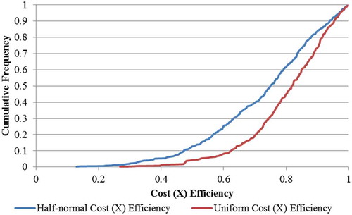
Figure 2. Frontier economies of scope cumulative frequency.

The economies of scope calculations for both the half-normal and uniform error distribution are identical.

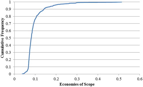
Figure 3. Frontier multi-product scale economies cumulative frequency for simulated data.

The MPSE calculations for both the half-normal and uniform error distribution are identical.

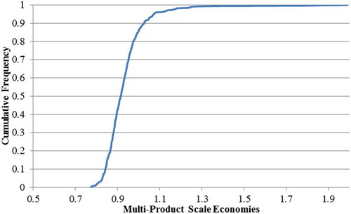
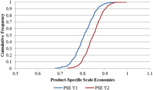
Figure 4. Frontier product-specific scale economies.

The PSE calculations for Y1 and Y2 for both the half-normal and uniform error distribution are identical.

While the CE for each firm is presented under a 500 observation uniform (500U) and a 500 observation half-normal distribution (500HN) (Figure 2), the SC, MPSE and PSEs from the frontier are identical for each data point (Table 3) due to the input prices (w_is) and output prices (p_is) being the same. Thus, the output quantities (y_is) remain unchanged (Equation 3).

A third data set is simulated using the same half-normal distribution but excluding the single output firms. In this set, there are 400 firms each producing both y₁ and y₂ (400HN). Structuring a simulation in this fashion examines each method’s ability to estimate an intercept similar in method with respect to DEA to Chavas and Aliber (1993) who proposed dropping any one output and associated costs and then re-estimating and repeating until each potential output has been dropped. Previous research has shown (Parman et al., 2017) that data sets with no single output firms are less accurate in estimating intercepts and incremental costs. However, in many industries, single and multiple output firms may not exist. Thus, this third data set is used to evaluate each method’s ability to estimate incremental costs and intercepts accurately when no firms exist producing one output or another.⁶

The difference between the “true” estimates and each of the four methods is evaluated by subtracting each model’s estimate from the “true” measure calculated with Monte Carlo simulation. A positive difference implies that the model underestimates the measure, and conversely, a negative difference indicates that the model overestimates the measure being evaluated. The mean absolute deviation is also reported for all four methods allowing for the comparison of average absolute deviation from zero.

Cumulative density functions are presented for the differences between the true measures and the estimated measures to provide visual representation of both bias and deviation. If there is no difference between the estimated measure and the true measure, the cumulative density function is a vertical line at zero.

3. Estimation methods

3.1. The two-sided error system equation

The traditional two-sided error system (Christensen et. al., 1973) involves specification of a cost function and single frontier of input quantities and costs from observed prices and outputs. This method fits a curve with observations residing above and below the estimated frontier. The cost function was estimated using the SHAZAM software package using a normalized quadratic cost function with input prices normalized on w₃ as⁷:

(5) $\begin{array}{rl}& C(W,Y)=b_0+\left[\begin{array}{cc}{b}_1& b_2\end{array}\right]\left[\begin{array}{c}{w}_1\\ w_2\end{array}\right]+\left[\begin{array}{cc}{a}_1& a_2\end{array}\right]\left[\begin{array}{c}{y}_1\\ y_2\end{array}\right]\\ & +\frac{1}{2}\left\{\left[\begin{array}{cc}{w}_1& w_2\end{array}\right]\left[\begin{array}{cc}{b}_{11}& b_{12}\\ b_{21}& b_{22}\end{array}\right]\left[\begin{array}{c}{w}_1\\ w_2\end{array}\right]+\left[\begin{array}{cc}{y}_1& y_2\end{array}\right]\left[\begin{array}{cc}{c}_{11}& c_{12}\\ c_{21}& c_{22}\end{array}\right]\left[\begin{array}{c}{y}_1\\ y_2\end{array}\right]\right\}+\left[\begin{array}{cc}{w}_1& w_2\end{array}\right]\left[\begin{array}{cc}{a}_{11}& a_{12}\\ a_{21}& a_{22}\end{array}\right]\left[\begin{array}{c}{y}_1\\ y_2\end{array}\right]+e_1\end{array}$(5)

(6) $\begin{array}{c}{x}_1=b_1+b_{11}{w}_1+b_{12}{w}_2+a_{11}{y}_1+a_{12}{y}_2+e_2\\ x_2=b_2+b_{12}{w}_1+b_{22}{w}_2+a_{21}{y}_1+a_{22}{y}_2+e_3\end{array}$(6)

The marginal costs are calculated by:

(7) $\begin{array}{c}mc{y}_1=a_1+c_{11}{y}_1+c_{12}{y}_2+a_{11}{w}_1+a_{21}{w}_2;and\\ mc{y}_2=a_2+c_{22}{y}_2+c_{12}{y}_1+a_{12}{w}_1+a_{22}{w}_2\end{array}$(7)

The incremental costs for each output are:

(8) $\begin{array}{c}IC{y}_1=a_1{y}_1+\frac{1}{2}{c}_{11}{y}_1^2+c_{12}{y}_1{y}_2+a_{11}{w}_1{y}_1+a_{21}{w}_2{y}_1;and\\ IC{y}_2=a_2{y}_2+\frac{1}{2}{c}_{22}{y}_2^2+c_{12}{y}_1{y}_2+a_{12}{w}_1{y}_2+a_{22}{w}_2{y}_2\end{array}$(8)

The costs of producing a single output are:

(9) $\begin{array}{c}C{Y}_1=C(W,Y)-IC{y}_2;and\\ C{Y}_2=C(W,Y)-IC{y}_1\end{array}$(9)

The economies of scope (SC), MPSE and product-specific scale economies (PSEy_i) can be calculated from the marginal costs, incremental costs and single output costs:

(10) $S{C}_i=\frac{\left[\sum _{i=1}^{2}C{Y}_i-C(W,Y)\right]}{C(W,Y)}$(10)

(11) $MPSE=\frac{C(W,Y)}{\left[\sum _{i=1}^{2}mc{y}_i\ast y_i\right]}$(11)

(12) $PSE{y}_i=\frac{IC{y}_i}{y_i\ast mc{y}_i}$(12)

CE measures are not calculated for the two-sided error system since the deviations from the “frontier” are two sided.

3.2. The OLS estimator with positive errors

A one-sided error model is estimated similar to the two-sided error model discussed above. However, a two-sided error model has errors above and below the frontier while a one-sided error model restricts the errors to be either above or below the frontier only. Also, the input demands in Equation (6) are not estimated in the one-sided error model. However, a two-sided error model has errors above and below the frontier while a one-sided error model restricts the errors to be either above or below the frontier only. Also, the input demands in Equation (6) are not estimated in the one-sided error model. with the difference being the error term is constrained to be positive and the input demand Equation (6) are not estimated. Equation (5) is estimated with the restriction that e_i ≥ 0 for all i using the General Algebraic Modeling Software (GAMS) program. The objective function minimizes the sum of squared errors subject to constraints that define the error. Firms on the frontier have errors equal to zero, while those with inefficiency exhibit positive errors. The calculations of SC, MPSE and PSE are identical to the two-sided error model using the coefficient estimates from the one-sided error model.

3.3. The stochastic frontier cost function estimator

The stochastic frontier estimation method uses FRONTIER Version 4.1 by Coelli (1991) based off of Battese and Coelli (1992) and Schmidt and Lovell (1979). One of the primary differences between the stochastic frontier method and the two methods above is the error term. Specifically, the error term consists of two elements, V_i which are random variables assumed to be iid N(0,σ²) and U_i which is a non-negative random variable capturing inefficiency. U_it is assumed to be half-normal for this analysis and defines how far above the frontier a firm operates. The resulting cost function is:

(13) $\begin{array}{rl}& C(W,Y)=b_0+\left[\begin{array}{cc}{b}_1& b_2\end{array}\right]\left[\begin{array}{c}{w}_1\\ w_2\end{array}\right]+\left[\begin{array}{cc}{a}_1& a_2\end{array}\right]\left[\begin{array}{c}{y}_1\\ y_2\end{array}\right]\\ & +\frac{1}{2}\left\{\left[\begin{array}{cc}{w}_1& w_2\end{array}\right]\left[\begin{array}{cc}{b}_{11}& b_{12}\\ b_{21}& b_{22}\end{array}\right]\left[\begin{array}{c}{w}_1\\ w_2\end{array}\right]+\left[\begin{array}{cc}{y}_1& y_2\end{array}\right]\left[\begin{array}{cc}{c}_{11}& c_{12}\\ c_{21}& c_{22}\end{array}\right]\left[\begin{array}{c}{y}_1\\ y_2\end{array}\right]\right\}+\left[\begin{array}{cc}{w}_1& w_2\end{array}\right]\left[\begin{array}{cc}{a}_{11}& a_{12}\\ a_{21}& a_{22}\end{array}\right]\left[\begin{array}{c}{y}_1\\ y_2\end{array}\right]+\left(V_i+U_i\right)\end{array}$(13)

For simplicity, Equation (13) can be rewritten as follows:

(14) $C(W,Y{)}_i=X_{i}B+\left(V_i+U_i\right)$(14)

The CE from the stochastic frontier method takes on a value between one and infinity since U_i ≥ 0. The CE from the nonparametric method and the one-sided error model is estimated by dividing the minimized total cost estimate by the actual total costs resulting in CE estimates between 0 and 1.

(15) $CE=\frac{X_{i}B}{X_{i}B+U_i}$(15)

The calculations of marginal costs, incremental costs, the SC, MPSEs and PSEs are the same as those shown above using the estimated parameters.

Each of the methods discussed above is parametric. Symmetry and homogeneity are imposed in the estimation process. Curvature and monotonicity are not imposed and would need to be examined to ensure that the cost function estimated is consistent with economic theory.

3.4. The nonparametric approach (DEA)

The nonparametric approach for estimating multi-product scale, product-specific scale and SC follows Parman et al. (2017). The cost (C_i) is determined for each firm where costs are minimized for a given vector of input prices (w_i) and outputs (y_i) with the choice being the optimal input bundle (x_i*).

(16) $\begin{array}{rl}& min{C}_i=w_i^{\prime }{x}_i^{\ast }\\ & s.t\\ & Xz\le x_i^{\ast }\\ & y^{\prime }z\ge y_p\\ & z_1+z_2+...+z_n=1\\ & z_i\in { }^{+}\end{array}$(16)

where there are “n” firms. The vector Z represents the weight of a particular firm with the sum of Z_is equal to 1 under variable returns to scale. From the above model, the minimum cost and output quantities can be estimated. The output quantities (y_p) constrain the cost minimizing input bundle to be at or above that observed in the data. Total cost from the model (C_i) is the solution to the cost minimization problem that produces a constrained minimum of each of the outputs for the ith firm. The cost of producing all outputs except one (C_i,all-p) where p represents the dropped output is determined by dropping the pth output constraint.

CE identifies a firm’s proximity to the cost frontier for a given output bundle and is the quotient of the estimated frontier cost (C_i) and the observed total cost (OTC_i) the firm incurred producing their output bundle.

(17) $C{E}_i=\left[\frac{C_i}{OT{C}_i}\right].$ (17)

The calculation for economies of scope is:

(18) $S{C}_i=\left[\frac{(\sum _p{C}_{i,p})-C_i}{C_i}\right].$(18)

The shadow prices on the output constraints (16) are the marginal cost of that output MC_i,p. MPSE is defined as:

(19) $MPS{E}_i=\left[\frac{C_{i,all}}{\sum _{p}M{C}_{i,p}{Y}_{i,p}}\right].$(19)

Product-specific economies of scale (PSE) require the calculation of the incremental costs (IC_i,p):

$I{C}_{i,p}=C_i-\sum _j{C}_{i,j\ne p}\mathrm{\forall }j.$

Average incremental costs (AIC_i,p) are determined by dividing incremental costs by the individual output:

$AI{C}_{i,p}=\frac{I{C}_{i,p}}{y_{i,p}}.$

Using the average incremental cost and the marginal cost calculations, the PSEs are:

(20) $PS{E}_{i,p}=\frac{AI{C}_{i,p}}{M{C}_{i,p}}.$(20)

When estimating the frontier nonparametrically using a data set with no observations of single output firms, the program will allow some of the output for the dropped constraint to be produced, resulting in an overstatement of the cost of that one output (C_i,p) which will cause an overstatement of economies of scope (Equation 18) and an understatement of product-specific scale economies (20). Thus, there exist additional product-specific production costs from an output being produced when, according to the economics theory, it should not be. The procedure for adjusting the costs in a two-goods case is as follows: the cost of producing y₁ only (C_i,1) assumes that only (y₁¹) is being produced. However, the optimization program allows some y_i,2¹ to be produced in this situation overstating the cost of producing y₁ only (C_i,1). To remove the additional cost, the percentage contribution of y_i,1¹ to cost is multiplied by the cost of producing y₁ only, yielding an adjusted cost (C^a_i,1). This estimated adjusted cost is used in the calculation of incremental costs and associated economic measures:

(21) $C_{i,1}^a=C_{i,1}\left(\frac{y_{i,1}^1}{y_{i,1}^1+y_{i,2}^2}\right)$(21)

This research evaluates the difference between the “true” measures of CE, economies of scope (SC), MPSE and product-specific economies of scale (PSE) from the four modeling approaches. The statistics and results presented are the difference between the model estimates and the “true” measure and not the economic measures.

The parametric estimators are specified knowing the “true” functional form: the normalized quadratic cost function. Therefore, the differences for the parametric methods may represent a “best case scenario” in that the true functional form is known and estimated with only the parameters being unknown.

4. Results

Table 4 contains the parameter estimates and standard errors for the parametric methods for all three data sets. The parameter estimates from each method are different under the same distributional assumptions and different for the same method under different distributional assumptions with the exception of the OLS-positive errors model that yielded the same parameter estimates for the uniform and half-normal distributions. For both the two-sided error system and the stochastic frontier estimation, different distributional assumptions yielded changes in magnitude as well as sign changes for various parameter estimates. Also, when comparing the 500U case to the 400HN with zero single output firms observed, there were changes for all three of the parametric methods as well as changes in magnitude for the estimated parameters. The calculation for the standard errors using GAMS used the method in Odeh, Featherstone, and Bergtold (1992).

Table 4. Parameter estimates and standard errors for three simulations of each parametric model.

	N = 500 half-normal (500HN)			N = 500 uniform (500U)			N = 400 (400HN)
	Two-sided errors	One-sided errors	Stochastic frontier	Two-sided errors	One-sided errors	Stochastic frontier	Two-sided errors	One-sided errors	Stochastic frontier
Price and output interaction parameters
A1	28.83 (4.67)	56.05 (3.61)	32.00 (27.32)	29.77 (2.05)	56.05 (1.88)	28.90 (3.74)	60.92 (23.12)	76.82 (5.24)	302.28 (12.03)
A2	79.33 (3.83)	88.39 (2.75)	46.05 (21.10)	80.18 (1.62)	88.39 (1.43)	78.24 (4.41)	52.38 (17.58)	54.74 (4.40)	−221.34 (10.46)
A11	0.49 (0.05)	−9.73 (2.42)	2.91 (19.55)	0.47 (0.04)	−9.73 (1.26)	3.04 (1.85)	1.17 (0.39)	24.21 (3.51)	−45.54 (22.64)
A12	0.67 (0.19)	−3.83 (1.39)	−7.58 (11.78)	0.56 (0.08)	−3.83 (0.72)	1.31 (1.57)	1.91 (0.75)	−16.74 (1.78)	−88.03 (21.90)
A21	0.54 (0.69)	−5.00 (1.71)	1.69 (14.72)	0.76 (0.03)	−5.00 (0.89)	4.45 (1.59)	0.12 (0.29)	−34.24 (2.71)	65.82 (18.24)
A22	−1.16 (0.15)	0.44 (1.13)	5.61 (9.84)	−0.39 (0.07)	0.44 (0.58)	1.66 (1.26)	−1.67 (0.59)	−0.99 (1.50)	78.41 (18.03)
Input price parameters and intercept
B0	684.95 (60.23)	360.20 (100.29)	−2011.12 (42.22)	401.01 (26.66)	360.20 (52.15)	460.56 (1.34)	689.81 (80.79)	−194.91 (42.64)	−4270.54 (1.82)
B1	26.18 (26.17)	−267.67 (104.00)	1833.84 (107.89)	20.20 (0.75)	−267.67 (54.07)	12.97 (1.17)	25.65 (1.74)	103.79 (46.62)	3225.37 (8.11)
B2	70.13 (5.25)	−200.80 (66.17)	825.29 (104.11)	57.29 (2.34)	−200.80 (34.40)	48.74 (1.71)	68.61 (4.74)	56.44 (26.04)	2109.47 (6.91)
B11	0.34 (0.18)	46.59 (89.08)	−834.08 (74.46)	−0.09 (0.08)	46.59 (46.36)	−65.45 (1.00)	0.12 (0.17)	−210.43 (34.17)	−529.61 (8.11)
B12	0.83 (0.51)	143.01 (34.06)	−297.13 (62.21)	0.20 (0.23)	143.01 (20.21)	−28.37 (1.05)	0.22 (0.50)	195.80 (14.26)	−1076.81 (10.09)
B22	2.85 (1.88)	27.48 (26.88)	−135.50 (114.14)	0.64 (0.87)	27.48 (14.90)	−8.34 (1.17)	0.25 (1.80)	2.74 (10.34)	−283.21 (13.61)
Output quantity parameters
C11	2.29 (0.15)	1.64 (0.18)	2.20 (1.25)	1.76 (0.06)	1.64 (0.09)	2.05 (0.50)	−0.35 (1.67)	−1.41 (0.64)	22.91 (13.05)
C12	−0.78 (0.53)	−0.25 (0.07)	0.10 (0.35)	−0.48 (0.02)	−0.25 (0.04)	−0.75 (0.19)	1.40 (1.25)	0.013 (0.53)	−15.66 (8.36)
C22	3.13 (0.68)	2.41 (0.12)	3.16 (0.78)	2.66 (0.04)	2.41 (0.06)	2.38 (0.32)	1.32 (0.97)	6.40 (0.43)	14.66 (5.63)

Curvature was checked for each parametric estimation method to ensure that it was not violated (Table 5). A curvature violation implies that the shape of the cost frontier estimation does not conform to the “true” cost function that is assumed and known in this case. This indicated that the parametric cost function violates economic theory conditions. To check these conditions, the eigenvalues are calculated for the “b” (price) and “c” (output) matrices where the eigenvalues for “b” should be negative (concave in prices) and “c” values should be positive (convex in outputs). Each parametric model violated curvature conditions for every simulation for either the “b” or “c” matrices or both. The one-sided error model and the two-sided system violated curvature conditions for both the “b” and “c” matrices for the 400HN observations simulation.

Table 5. Eigenvalues for “B” (prices) and “C” (outputs) matrices for each model and simulation.

Half-normal (500HN)		Uniform (500U)		No zero outputs (400HN)
B	C	B	C	B	C
Two-sided error system
3.09	3.50	0.70	2.80	0.41	2.10
0.09	1.80	−0.10	1.50	−0.40	−1.14
X	√	X	√	X	X
Stochastic frontier
−37.0	3.20	3.10	2.90	677	34.8
−931	−2.20	−76.0	1.40	−1489	2.60
√	X	X	√	X	√
OLS-positive errors
180	2.40	180	2.40	118	6.00
−106	1.50	−106	1.50	−325	−1.50
X	√	X	√	X	X

The known cost function is concave in prices (B matrix) and convex in outputs(C matrix). For concavity, the matrix must yield negative eigenvalues, and for convexity, the matrix must yield positive eigenvalues. A “√” implies correct curvature, while “X” implies a curvature violation.

4.1. Cost efficiency

CE differences determine the ability of each model to estimate the “true” frontier since it is the ratio of estimated minimum cost to actual total cost. The two-sided error model was not examined because it is not a frontier function. The OLS-positive errors and nonparametric models performed well for all three data sets in estimating the frontier with average differences below 0.03 in absolute value and standard deviations below 0.04 (Table 6). The most accurate estimation of CE was the nonparametric model under the uniform distribution simulation with the average, standard deviation and mean absolute deviation close to zero.

Table 6. Statistics for simulated cost efficiency differences (CE) for the OLS-positive errors, stochastic frontier and nonparametric estimations.

	Average	Standard deviation	Minimum	Maximum	Mean absolute deviation
Half-normal distribution (500HN)
OLS-positive errors	−0.020	0.039	−0.277	0.063	0.023
Stochastic frontier	−0.015	0.043	−0.304	0.155	0.024
Nonparametric	−0.025	0.041	−0.530	−0.003	0.026
Uniform distribution (500U)
OLS-positive errors	−0.011	0.013	−0.062	0.122	0.013
Stochastic frontier	−0.198	0.118	−1.478	−0.058	0.198
Nonparametric	−0.004	0.007	−0.079	0.000	0.004
400 observations (400HN)
OLS-positive errors	−0.017	0.023	−0.173	0.015	0.017
Stochastic frontier	−0.028	0.049	−0.351	0.139	0.039
Nonparametric	−0.022	0.032	−0.386	−0.003	0.022

The stochastic frontier method performed almost as well under the 500HN simulation with the average closest to zero and under the 400HN observation simulation with an average difference of −0.028 but much worse under the 500U (Figure 5) with an average difference of −0.198, mean absolute deviation of 0.198 and standard deviation of 0.118. This implies that estimating efficiency measures with the stochastic frontier method is dependent on the correct assumption of the inefficiency error distribution when inefficiency is symmetrically distributed. However, other research shows that in the case of asymmetric and skewed distributions such as the truncated normal, half-normal and exponential, that distributional assumptions are much less impactful (Meesters, 2014).

Figure 5. Differences between frontier cost efficiency and estimated cost efficiency for the nonparametric, frontier and OLS-positive errors models.

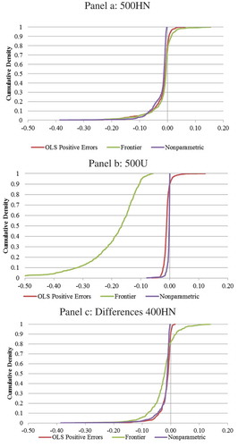
In all cases, the average differences were below zero implying that the OLS-positive errors, stochastic frontier and nonparametric models slightly overestimated the CEs for most of the firms. This is confirmed by examining the mean absolute deviation in the 500U and 400HN observations cases being the same as the absolute value of the mean. Frontier methods envelope the observed data, thus CEs are overestimated unless there are a significant number of firms where the simulated error is zero. The average differences were close to zero in most cases with low standard deviations.

4.2. Economies of scope

Differences in estimates of economies of scope for the four different methods were not as accurate as the CE estimates. For both the 500HN and 500U simulations, the two-sided error system had an average error that was furthest from zero at −0.30 with a standard deviation similar to the other methods (Table 7). For the 400HN simulation, the average error for the stochastic frontier method was furthest from zero at −2.32. Due to scaling, the stochastic frontier method cumulative density is not visible in Figure 6 for the 400HN case.

Table 7. Statistics for economies of scope (SC) differences from all four methods from all three data sets.

	Average	Standard deviation	Minimum	Maximum	Mean absolute deviation
Half-normal distribution (500HN)
Two-sided error system	−0.300	0.057	−0.474	−0.194	0.300
OLS-positive errors	−0.082	0.067	−0.291	0.093	0.088
Stochastic frontier	−0.101	0.056	−0.266	0.052	0.103
Nonparametric	−0.089	0.030	−0.249	0.029	0.089
Uniform distribution (500U)
Two-sided error system	−0.300	0.058	−0.489	−0.191	0.300
OLS-positive errors	0.010	0.023	−0.044	0.190	0.018
Stochastic frontier	−0.158	0.041	−0.312	−0.091	0.158
Nonparametric	−0.019	0.079	−0.904	0.017	0.020
400 observations (400HN)
Two-sided error system	−0.148	0.115	−0.437	0.152	0.175
OLS-positive errors	−0.187	0.053	−0.376	−0.048	0.187
Stochastic frontier	−2.324	0.607	−4.109	−0.142	2.324
Nonparametric	0.070	0.036	0.025	0.514	0.070

Figure 6. Differences between frontier economies of scope and estimated economies of scope from two-sided errors, OLS-positive errors, frontier and nonparametric models.

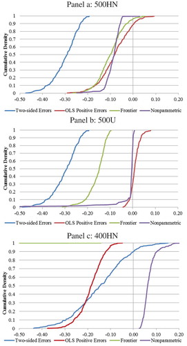
The OLS-positive errors model and nonparametric model estimated economies of scope closely with averages for the 500HN of −0.08 and −0.09, respectively, and standard deviations around 0.07 and 0.03, respectively (Table 7). The estimates of scope for the 500U distribution from the OLS-positive errors model and nonparametric model were less than 0.02 in absolute value with low standard deviations. The average and standard deviation for the nonparametric method under the 500U simulation were affected by a few observations (Figure 6). For the 400HN data set, the nonparametric method had the lowest standard deviation (0.04) and an average closest to zero in absolute value (0.07) (Table 7).

The three parametric estimation methods overestimated economies of scope in each of the simulations except for the case of a half-normal distribution where the OLS-positive errors model underestimated the economies of scope slightly. In many cases, the parametric methods strictly overestimated scope in that the absolute values of the means were the same as the mean absolute deviations (Table 7). The nonparametric model slightly overestimated scope in both the 500HN and 500U simulations but slightly underestimated scope in the 400HN data set.

The most robust estimator of economies of scope appears to be the nonparametric approach with averages close to zero in all three simulations and low standard deviation. The OLS-positive errors model does not perform as well in the case of the 400HN simulation, nor does the stochastic frontier model and the standard two-sided error system under the 500HN and 500U simulations. Measures of economies of scope become suspect using any of the methods when there are no single output firms in the data sample. None of the methods extrapolate well out-of-sample.

4.3. Multi-product economies of scale

An accurate estimation of MPSE requires both a close approximation of the true frontier and marginal costs. It is possible to have a good approximation for the MPSE but not for economies of scope and PSEs due to the estimation of incremental costs necessary for scope and the PSE measures.

The nonparametric approach appears to be the most robust estimator of MPSE (Figure 7). It has an average difference closest to zero in all three simulations and the lowest standard deviation in both the 500HN and 400HN cases (Table 8). Its mean absolute deviation is also lowest except compared to the OLS-positive errors model under the 500U distribution. The standard deviation was only slightly higher for the nonparametric approach compared to the OLS-positive errors model in the 500U case with a standard deviation of 0.05 for the nonparametric model and 0.04 for the OLS-positive errors model (Table 8). All average differences except OLS-positive errors in the 500U case were negative implying that MPSE was, for the most part, overestimated by the models.

Table 8. Statistics for multi-product scale economies (MPSE) differences from all four methods from all three data sets.

	Average	Standard deviation	Minimum	Maximum	Mean absolute deviation
Half-normal distribution (500HN)
Two-sided error system	−0.443	0.361	−2.917	−0.067	0.443
OLS-positive errors	−0.257	0.658	−5.995	0.104	0.272
Stochastic frontier	−0.084	0.183	−1.577	0.107	0.107
Nonparametric	−0.002	0.096	−0.678	0.739	0.049
Uniform distribution (500U)
Two-sided error system	−0.482	0.609	−7.857	−0.068	0.482
OLS-positive errors	0.023	0.044	−0.124	0.515	0.027
Stochastic frontier	−0.210	0.258	−3.384	−0.030	0.210
Nonparametric	−0.012	0.054	−0.277	0.114	0.029
400 observations (400HN)
Two-sided error system	−0.371	0.300	−4.642	−0.065	0.371
OLS-positive errors	−0.087	0.131	−1.331	0.105	0.103
Stochastic frontier	−0.074	0.152	−0.727	0.177	0.118
Nonparametric	−0.009	0.137	−0.821	0.743	0.058

Figure 7. Differences between frontier multi-product scale economies and estimated multi-product scale economies from the two-sided errors, OLS-positive errors, frontier and nonparametric models.

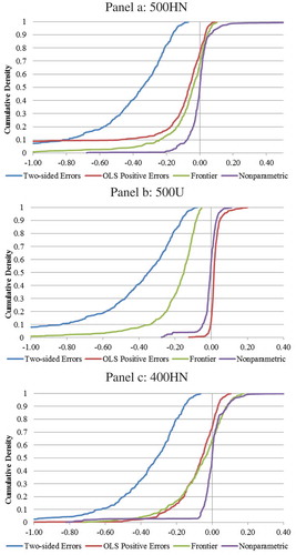
Of the four modeling methods in all three simulations, the two-sided error system had the largest average differences from zero and the highest standard deviations (Table 8). No observations were correctly estimated for MPSE (Figure 7) in any of the three simulations. Using the standard two-sided system approach, the error never approaches the zero difference.

The stochastic frontier method results were mixed. While it was outperformed by the nonparametric approach in each of the simulations, it was close to the “true MPSE” in the case of the 400HN simulation. However, in the 500U simulation, it did not perform well with an average difference of −0.21 and standard deviation of 0.26 (Table 8).

4.4. Product-specific economies of scale

The estimation of the PSEs for both y₁ and y₂ for the 500HN and 500U simulations yielded similar results for all three parametric-type estimations (Table 9). The parametric approaches appear to slightly outperform the nonparametric approach in the estimation of PSE₁ (Figure 8a, left) in the half-normal simulation but performed similarly in the estimation of PSE₂ (Figure 8b, left) under the same distribution in terms of absolute distance from zero. For the 500U simulation, the PSE₁ and PSE₂ estimates from the nonparametric model were similar to both the stochastic frontier method and the two-sided error systems with the OLS-positive errors model being the closest to zero under the 500U simulation (Table 9).

Table 9. Statistics for product-specific scale economies (PSE) differences for y₁ and y₂ from all four methods and all three data sets.

		Average	Standard deviation	Minimum	Maximum	Mean absolute deviation
	Half-normal distribution (500HN)
	Two-sided error system	0.099	0.024	0.047	0.147	0.099
y1	OLS-positive errors	−0.056	0.039	−0.130	0.140	0.064
	Stochastic frontier	0.111	0.018	0.081	0.176	0.111
	Nonparametric	0.128	0.202	−0.259	0.573	0.202
	Two-sided error system	0.053	0.011	0.022	0.081	0.053
y2	OLS-positive errors	0.075	0.016	0.037	0.148	0.075
	Stochastic frontier	0.060	0.006	0.004	0.072	0.060
	Nonparametric	0.027	0.099	−0.344	0.303	0.085
	Uniform distribution (500U)
	Two-sided error system	0.098	0.025	0.024	0.147	0.098
y1	OLS-positive errors	0.012	0.013	−0.012	0.049	0.013
	Stochastic frontier	0.056	0.018	0.012	0.093	0.056
	Nonparametric	0.020	0.123	−0.241	0.299	0.097
	Two-sided error system	0.052	0.011	0.002	0.075	0.052
y2	OLS-positive errors	0.005	0.002	0.000	0.011	0.005
	Stochastic frontier	0.004	0.004	−0.008	0.012	0.005
	Nonparametric	−0.004	0.053	−0.186	0.126	0.039
	400 observations (400HN)
	Two-sided error system	−0.218	0.054	−0.368	−0.048	0.218
y1	OLS-positive errors	−0.421	0.296	−4.110	−0.066	0.421
	Stochastic frontier	1.696	32.94	−619.9	120.5	6.480
	Nonparametric	0.187	0.310	−0.311	0.957	0.266
	Two-sided error system	−0.036	0.015	−0.086	0.000	0.036
y2	OLS-positive errors	0.302	0.028	0.042	0.373	0.302
	Stochastic frontier	−9.224	248.9	−4952	444.3	18.15
	Nonparametric	0.132	0.209	−0.248	0.937	0.183

Figure 8. Differences between frontier product-specific scale economies for Y_i and estimated product-specific scale economies for Y_i from the two-sided errors, OLS-positive errors, frontier and nonparametric models.

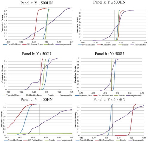
Under the 500HN and the 500U simulations, the two-sided error system and the stochastic frontier underestimated PSEs for y₁ and y₂. The OLS-positive errors model underestimated PSEs under both distributions except for the 500HN PSE₁. In the 400HN simulation, OLS overestimated both PSEs where that was not the case for the nonparametric model and OLS-positive errors model.

The average difference and standard deviation for the PSEs from the stochastic frontier method in the 400HN simulation are estimated poorly (Table 9). Of the parametric methods, it appears that two-sided error system performed best when there were no single output firms having the lowest standard deviations and averages fairly close to zero, especially for PSE₂ (Figure 8b, right).

In the 400HN simulation, while the standard deviation was higher for the nonparametric method than OLS and OLS-positive errors, the average for PSE₁ was closest to zero using the nonparametric method and closer than OLS-positive errors and the stochastic frontier method for PSE₂ (Table 9). None of the methods accurately predict the PSEs when there were no single output observations (Figure 8c).

The challenge for each method in the 400HN simulation is that there are no firms producing a single output. This requires each method to extrapolate estimates out of sample for the purpose of calculating incremental costs. If the smallest firms are not efficient, a linear projection is inaccurate depending on the amount of inefficiency of the firms.

5. Summary and conclusions

Four methods for estimating a cost frontier and associated economic measures were examined under three different simulations including a half-normal distribution inefficiency, a uniform inefficiency distribution, and a data set with no single output firms observed. The four methods examined were a traditional two-sided error system regression with costs residing above and below the fitted curve, the stochastic frontier method proposed by Aigner et al. (1977) where the error term ensures all observations lie on or above the cost frontier, an OLS regression method where the error term was restricted to take on positive values only ensuring that all observations lie on or above the cost frontier and a nonparametric method proposed by Färe et al. (1985) using a series of linear segments to trace out the cost frontier. For each simulation, CE, economies of scope, MPSE and product-specific scale economies were calculated and compared to the known values from the “true” cost frontier.

Results suggest that the two-sided error system is the least accurate method for estimating a frontier function and associated cost measures. This empirical method lacks consistency with the economic definition of a cost frontier, and it does not, in any simulation, robustly estimate the MPSE or economies of scope.

The OLS-positive errors model appears to accurately project the cost frontier regardless of the distributional assumption and whether there are no single output firms observed. However, like the stochastic frontier method, the OLS-positive errors method has difficulty extrapolating incremental costs when there are no single output firms (400HN). Thus, under no single output cases, the economies of scope estimations from the positive errors model may be inaccurate along with the PSE estimates.

The stochastic frontier method appears susceptible to inaccurate distributional assumptions on the one-sided error as it estimates the frontier much closer to the “true” frontier under a half-normal distribution (500HN) rather than the uniform distribution (500U) when assuming that the true distribution is a half-normal estimation process. Results also suggest that the stochastic frontier method has difficulty extrapolating when there are no single output firms observed in the data as indicated by its inability to accurately estimate economies of scope or PSEs for the no single output firms simulation (400HN). However, in the case of a half-normal error distribution (500HN) (the “true” distribution), it accurately estimates the frontier and, with the existence of single output firms in the sample, accurately estimates economies of scope and PSEs.

The nonparametric method in all three simulations is fairly robust in estimating the “true” cost frontier and associated economic measures. It is also the model most capable of handling data with no single output firms observed due to its proximity to zero in estimating economies of scope and PSEs. It does not appear to be particularly susceptible to distributional assumptions on inefficiency.

All of the parametric methods assumed the functional form of the “true” frontier (normalized quadratic) in the estimation process. Thus, these results may be different if the true functional form differs from the function form assumed in the estimation of the parametric methods. Functional form and statistical assumptions are not necessary in the case of the nonparametric method; thus, this method may be more robust when the true functional form and the distribution of efficiency are unknown. That is, if a researcher is unsure of model specification or the inefficiency distribution, the nonparametric approach may be a good alternative to parametric methods.

The results show that the three frontier estimators were capable of estimating the “true” frontier in some cases. However, the stochastic frontier method was as robust as neither the nonparametric method nor the OLS-positive errors model in the estimation of MPSE. All three frontier methods estimated the zero single output firms data simulation and the half-normal simulation fairly close; however, the stochastic frontier model was not as close when inefficiency was distributed uniform as when the estimation method assumed a half-normal distribution. The OLS method with two-sided errors was the furthest from the “true” calculation of MPSE, indicating that it was not accurate in estimating marginal cost.

Overall, the nonparametric approach estimated the frontiers and associated economic measures close to the “true” values considering that no special assumptions or specifications were required in its estimation. Its estimation of the frontier was about as close or closer to the “true” values as any of the methods examined and its calculations of economies of scope and MPSE were the closest in several of the scenarios presented. The nonparametric approach did not significantly fail to estimate PSEs compared to any other method. Therefore, it appears that the nonparametric method is robust for estimating scale and scope measures.

Disclosure statement

No potential conflict of interest was reported by the authors.

Additional information

Notes on contributors

Bryon J. Parman

Bryon J. Parman is an assistant professor in the Department of Agribusiness and Applied Economics at North Dakota State University. He received his Ph.D. from Kansas State University. His areas of specialty are agricultural economics and agribusiness production and finance.

Allen M. Featherstone

Allen M. Featherstone is a professor and head of agricultural economics at Kansas State University. He received his Ph.D. from Purdue University. His areas of specialty are agricultural economics and the theory of the firm.

Notes

¹ Frontier V4.1 written by Tim Coelli is available online at: http://www.uq.edu.au/economics/cepa/frontier.php.

² The analysis also was completed for alternative assumptions on input prices.

³ The analysis also examined the alternative standard deviations.

⁴ The analysis also examined alternative numbers of observations. The results were invariant to 500 and 2,500 observations.

⁵ The goal of this method is to ensure that single output firms are in the sample. This assumption is further relaxed to determine the robustness of the alternative methods to a situation where no single output firms are observed in the data. Examining data with single output firms and with no single output firms is also a check on the accuracy of incremental cost estimates needed for the economic effects of scope and product-specific economies of scale.

⁶ See Parman et al. (2017) for comparisons of dropping outputs vs. constraining them to zero in the DEA framework.

⁷ It should be noted that for each of the parametric methods, the true functional relationship is provided. That is, in each of the parametric cases, the quadratic functional form is used. While not being known in actual applications, this will benefit the results from the parametric methods when compared to the DEA method.

References

- Afriat, S. N. (1972). Efficiency estimation of production functions. International Economic Review, 13(3), 568–598.
- Aigner, D. J., Lovell, C. A. K., & Schmidt, P. (1977). Formulation and estimation of stochastic frontier production models. Journal of Econometrics, 6, 21–37.
- Andor, M., & Hesse, F. (2013). The StoNED age: The departure into a new era of efficiency analysis? A Monte Carlo comparison of StoNED and the “Oldies” (SFA and DEA). Journal of Productivity Analysis, 41, 85–109.
- Assaf, A., & Matawie, K. M. (2010). Improving the accuracy of DEA efficiency analysis: A bootstrap application to the health care foodservice industry. Applied Economics, 42(1), 3547–3558.
- Badunenko, O., Henderson, D. J., & Kumbhakar, S. C. (2012). When, where, and how to perform efficiency estimation. Journal of the Royal Statistical Society: Series A (Statistics in Society), 175(4), 863–892.
- Battese, G., & Coelli, T. (1988). Prediction of firm-level technical efficiencies with a generalized frontier production function and panel data. Journal of Econometrics, 38, 387–399.
- Battese, G., & Coelli, T. (1992). Frontier production functions, technical efficiency and panel data. With application to paddy farmers in India. Journal of Productivity Analysis, 3, 153–169.
- Bojani, A. N., Caudill, S. B., & Ford, J. M. (1998). Small-sample properties of ML, COLS, and DEA estimators of frontier models in the presence of heteroscedasticity. European Journal of Operational Research, 108(1), 140–148.
- Charnes, A., Cooper, W. W., & Rhodes, E. (1978). Measuring the efficiency of decision making units. European Journal of Operational Research, 9, 181–185.
- Chavas, J.-P., & Aliber, M. (1993). An analysis of economic efficiency in agriculture: A nonparametric approach. Journal of Agricultural and Resource Economics, 18, 1–16.
- Christensen, L. R., Jorgenson, D. W., & Lau, L. J. (1973). Transcendental logarithmic production frontiers. The Review of Economics and Statistics, 55(1), 28–45.
- Coelli, T. (1991). Maximum likelihood estimation of stochastic frontier Production functions with time varying technical efficiency using the computer program FRONTIER version 2.0. Armidale, Australia: Department of Economics, University of New England.
- Diewert, W. E., & Wales, T. J. (1988). A normalized quadratic semiflexible functional form. Journal of Econometrics, 37(3), 327–342.
- Färe, R., Groskopf, S., & Lovell, C. A. K. (1985). The measurement of efficiency of production. Boston: Kluwer-Nijhoff.
- Farrell, M. J. (1957). The measurement of productive efficiency. Journal of the Royal Statistical Society, 120(3), 253–290.
- Farrell, M. J., & Fieldhouse, M. (1962). Estimating efficient production under increasing returns to scale. Journal of the Royal Statistical Society, 125(2), 252–267.
- Featherstone, A. M., & Moss, C. B. (1994). Measuring economies of scale and scope in agricultural banking. American Journal of Agricultural Economics, 76(3), 655–661.
- Fried, H. O., Knox Lovell, C. A., & Schmidt, S. S. (2008). The measurement of productive efficiency and productivity growth. Chapter 8 (William H. Greene) (pp. 94–249). New York, NY: Oxford University Press, Inc.
- Gao, Z., & Featherstone, A. M. (2008). Estimating economies of scope using the profit function: A dual approach for the normalized quadratic profit function. Economic Letters, 100, 418–421.
- Gong, B.-H., & Sickles, R. (1992). Finite sample evidence on the performance of stochastic frontiers and data envelopment analysis using panel data. Journal of Econometrics, 51(1–2), 259–284.
- Green, W. (1997). Handbook of applied econometrics: Microeconomics vol 2, Blackwell handbooks in economics. Wiley-Blackwell.
- Greene, W. (2005). Efficiency of public spending in developing countries: A stochastic frontier approach. Stern School of Business, New York University. 44 West 4th Street, New York, NY.
- Hjalmarsson, L., Kumbhakar, S. C., & Heshmati, A. (1996). DEA, DFA and SFA: A comparison. Journal of Productivity Analysis, 7(2–3), 303–327.
- Kuosmanen, T., & Kortelainen, M. (2012). Stochastic non-smooth envelopment of data: Semi-parametric frontier estimation subject to shape constraints. Journal of Productivity Analysis, 38(1), 11–28.
- Kuosmanen, T., Saastamoinen, A., & Sipiläinen, T. (2013). What is the best practice for benchmark regulation of electricity distribution? Comparison of DEA, SFA and StoNED methods. Energy Policy, 61, 740–750.
- Lee, S., & Lee, Y. H. (2014). Stochastic frontier models with threshold efficiency. Journal of Productivity Analysis, 42, 45–54.
- Li, Q. (1996). Estimating a stochastic production frontier when the adjusted error is symmetric. Economic Letters, 52(3), 221–228.
- Lusk, J. L., Featherstone, A. M., T. L., & Abdulkadri, A. O. (2002). The empirical properties of duality theory. The Australian Journal of Agricultural and Resource Economics, 46, 45–68.
- Mas-Colell, A., Whinston, M. D., & Green, J. R. (1995). Microeconomic theory. New York, NY: Oxford University Press.
- Meesters, A. (2014). A note on the assumed distributions in stochastic frontier models. Journal of Productivity Analysis, 42(2), 171–173.
- Meeusen, W., & Van Den Broeck, J. (1977). Efficiency estimation from Cobb-Douglas production functions with composed error. International Economic Review, 18, 435–444.
- Odeh, O. O., Featherstone, A. M., & Bergtold, J. S. (1992). Reliability of statistical software. American Journal of Agricultural Economics, 5, 1472–1489.
- Parman, B. J., Featherstone, A. M., & Coffey, B. K. (2017). Estimating product-specific and multiproduct economies of scale with data envelopment analysis? Journal of Agricultural Economics, 48, 1–11.
- Parmeter, C. F., & Kumbhakar, S. C. (2014). Efficiency analysis: A primer on recent advances. Foundations and Trends in Econometrics, 7(3–4), 191–385.
- Paul, C. M., Nehring, R., Banker, D., & Somwaru, A. (2004). Scale economies and efficiency in U.S. agriculture: Are traditional farms history? Journal of Productivity Analysis, 22, 185–205.
- Richmond, J. (1974). Estimating the efficiency of production. International Economic Review, 15, 167–182.
- Ruggiero, J. (1999). Efficiency estimation and error decomposition in the stochastic frontier model: A Monte Carlo analysis. European Journal of Operational Research, 129, 434–442.
- Ruggiero, J. (2007). A comparison of DEA and the stochastic frontier model using panel data. International Transactions in Operational Research, 14, 259–266.
- Schmidt, P., & Lovell, C. (1979). Estimating technical and allocative inefficiency relative to stochastic production and cost frontiers. Journal of Econometrics, 9(3), 343–366.
- Simar, L., & Wilson, P. W. (1998). Sensitivity analysis of efficiency scores: How to bootstrap in nonparametric frontier models. Management Science, 44(1), 49–61.
- Simar, L., & Wilson, P. W. (2013). Estimation and inference in nonparametric frontier models: Recent developments and perspectives. Foundations and Trends in Econometrics, 5(3–4), 183–337.
- Thanassoulis, E. (1993). A comparison of regression analysis and data envelopment analysis as alternative methods for performance assessments. Journal of the Operational Research Society, 44(11), 1129–1144.