Modeling past and future variation of glaciers in the Dongkemadi Ice Field on central Tibetan Plateau from 1989 to 2050

ABSTRACT

Glacier mass balance change is among the best indicators of glacier response to climate change. Due to its inaccessibility and limited observation, little is known about the change to the Dongkemadi Ice Field (DIF) in the Tanggula Mountains located in the source region of the Yangtze River in central Tibetan Plateau. Here, an enhanced temperature index–based glacier model considering glacier area change was applied to study the temporal–spatial variation in mass balance on the DIF from 1989 to 2012 and to assess its response to climate change. The model was forced by reconstructed temperature and precipitation from adjacent national meteorological stations and validated by comparing with field observations from the Xiao Dongkemadi Glacier (XDG). Results show that the simulated mass balance is in good agreement with the observations (R² = 0.75, p < .001), and the model can reasonably reproduce well the glacier mass change. Then the model was applied to twenty individual glaciers in DIF and forced by the high-resolution regional climate model (RegCM3) from 2013 to 2050 to project their further variation. In the future, the mass balance of glaciers in DIF shows a continuously negative trend with a linear rate of −0.16 m water equivalent (w.e.) a⁻¹ in representative concentration pathway (RCP) 4.5 and −0.35 m w.e. a⁻¹ in RCP 8.5. Most of the glaciers’ equilibrium line altitudes (ELAs) will reach or exceed their maximum elevation after the 2030s. By coupling a modified volume–area scaling method with the mass balance model, results showed that areas of the individual glaciers in DIF will lose about 12.10 to 30.66 percent under RCP4.5 and 14.06 to 38.76 percent under RCP8.5, and the volume of the DIF will lose about 1.18 km³ in RCP4.5 and 1.44 km³ in RCP8.5 by the end of 2050. In addition, the terminuses of glaciers experienced the largest percentage losses and most of the glaciers’ front position will reach ~5,520 m a.s.l. in RCP 4.5 and 5,570 m a.s.l. in RCP 8.5, the latter of which is nearly close to the DIF average ELA in 1989. The clearly increasing summer air temperature may be the main reason for glacier shrinkage in the DIF. If the warming trend continues, glaciers in DIF may further retreat with continued glacial melt or even mostly disappear by the end of the century.

KEYWORDS:

• Dongkemadi Ice Field
• temperature index model
• glacier mass balance
• climate change
• volume–area scaling method

Introduction

As an important freshwater resource, glaciers play an essential role in the global water cycle as hydrological reservoirs at various timescales (Immerzeel, van Beek, and Bierkens 2010). However, the majority of glaciers around the world have decreased, with an accelerated retreat trend during the past several decades because of global climate warming (Bliss, Hock, and Radić 2014; Radić et al. 2014). Mountain glaciers are experiencing more serious retreat due to their higher sensitivity to changes in climate forcing (Bonanno et al. 2014; L. Wang et al. 2014). These changes will eventually endanger the existence of oasis cities and terminal lakes in the longer term, especially in arid and semiarid areas, such as those in western China (Yao et al. 2004).

The Tibetan Plateau (TP) has more than 40,000 mountain glaciers (Guo et al. 2015), and most of them have been shrinking and thinning at an accelerated rate during the past two decades, as reported from in situ measurements and remote sensing studies (Bolch et al. 2012; Yao et al. 2012; M. Yang et al. 2019). However, patterns of glacier change (e.g., climatic mass balance) have great spatial heterogeneity under different climate regimes (Jacob et al. 2012; Kääb et al. 2012). For example, It has been observed that rates of mass loss are greatest for maritime glaciers and lower for continental glaciers (Yao et al. 2012; M. Yang et al. 2019). Furthermore, several glaciers have remained stable or even advanced in some regions; for example, the western Himalayas (H. Zhao et al. 2016) and the Karakoram (Gardelle, Berthier, and Arnaud 2012; Forsythe et al. 2017). The fundamental mechanisms controlling these spatial patterns are still under debate (Fujita and Nuimura 2011; Scherler, Bookhagen, and Strecker 2011; Gardelle, Berthier, and Arnaud 2012; Yao et al. 2012), indicating that the response of glaciers to climate change on the TP is complex (Fujita 2008; Rupper and Roe 2008; Mölg, Maussion, and Scherer 2014). Moreover, because the magnitude of climate change on the TP is not uniform (D. Zhang et al. 2013; Kuang and Jiao 2016), the spatial heterogeneity of glacier variation in the future with global temperature rise will increase. But how and to what extent the glaciers will respond to climate change, and what impacts glacier change will have on the local and downstream water resources, is still not clear.

Glacier mass balance directly connects climate change and glaciers (Bolch et al. 2012), and modeling is the major method for assessing variation in glacier mass balance, especially for future projections (Pellicciotti et al. 2005; Reijmer and Hock 2008; Hock, Hutchings, and Lehning 2017). However, sufficient input data for comprehensive modeling of glacier mass variation are available for a limited number of well-studied (and almost all small) glaciers on the TP; for example, No. 1 Glacier at the source of Urumqi River and Qiyi Glacier (Yao et al. 2012; S. Wang et al. 2017). For most of the glaciers on TP, simpler models are better alternatives due to the data limits. One widely adopted approach includes temperature index models (Hock 1999; Pellicciotti et al. 2005), which rely on the empirical relationships between ice melts and positive temperatures (Huss et al. 2008). Theoretically, this type of model is based on the high correlation between certain components of the energy balance (longwave incoming radiation and sensible heat flux) and air temperature (Ohmura 2001). To improve the accuracy of simulation, glacier area change, clear sky radiation, and shading effects are also considered in such a model (Hock 1999, 2003). After several rounds of improvements, the present model has satisfactory performance with limited input data (Hock, Hutchings, and Lehning 2017), especially for the period for which calibration data are available (Hock 1999; Pellicciotti et al. 2005). Performance is often better than that of energy–mass balance models (Gabbi et al. 2014; S. Wang et al. 2017), especially for glacier projection (Réveillet et al. 2018). Thus, to explore the mechanisms of glacier response to climate change and project its future possible variation, a temperature index model is the best choice for the study area.

Dongkemadi Ice Field (DIF) is located at the headwaters of the Yangtze River (Fujita, Ohta, and Ageta 2007; Pu et al. 2008; Z. Li et al. 2012), contributing about 17 percent to river runoff since the 1990s (S. Liu et al. 2009). As an important regional source of water, it is also important for local residents and alpine wildlife (S. Wu et al. 2013; Z. Zhang et al. 2018). Thus, understanding the mass balance evolution of glaciers in the DIF is of great interest. However, few detailed studies are available on the glacier mass balance process in the DIF due to its inaccessibility and limited observations. Earlier works studied glacier mass change based on remote sensing (Z. Li et al. 2012; G. Liu et al. 2015; Z. Zhang et al. 2018) and in situ observations of individual small glaciers (Fujita et al. 2000; Pu et al. 2008; Shangguan et al. 2008; Y. Yang, Li, et al. 2016). However, previous research focused on a short and fragmented time range, missing temporal information on long-term mass balance change in the DIF. In addition, although a few studies have tried to establish a model for long-term change for individual glaciers in the DIF (P. Shi et al. 2016), it remains impossible to construct a model for continuous long-term variation for the whole DIF. Thus, there is a knowledge gap regarding the regional response of glaciers to climate change in the DIF area and the impact of glacier melt on the local and downstream regions. In addition, the future impacts of possible evolution and glacier melt on water resources remain unknown due to the lack of modeling work in the area.

To address these issues, we selected Xiao Dongkemadi Glacier (XDG) in the DIF as a representative glacier and reconstructed the seasonal mass balance variation from 1989 to 2012 using a distributed enhanced temperature index model. Based on the calibrated parameters obtained from the XDG, we spatially extrapolated the model to twenty climatologically similar glaciers in the DIF to calculate the variation in mass balance for the whole DIF. Then, using a coupled modified volume–area (V-A) scaling method (Marzeion, Jarosch, and Hofer 2012; Bahr, Pfeffer, and Kaser 2015), the ongoing recession of the glacier area, volume, and terminus elevation were calculated. Finally, combining with downscaled climate data, we projected the DIF variation under representative concentration pathway (RCP) 4.5 and RCP 8.5 scenarios (2013–2050) and assessed its response to global climate change. The results may help us understand the regional response of glacier melt to climate change and provide an impetus for further handling of water reserves.

Study site and field data

Research area

The DIF is located in the middle of the Tanggula Mountain range (33°00′–33°06′ N, 91°58′–92°06′ E) in the central TP with a mean elevation above 5000 m a.s.l. (Figure 1), covering a total area of over 80 km² according to the Second Glacier Inventory of China (Guo et al. 2015). It is one of the major source regions of the Yangtze River in western China and provides fresh water for the local area and downstream regions (S. Liu et al. 2009). As a typical continental glacier, it is primarily controlled by continental/subcontinental climate conditions and is less influenced by the midlatitude westerlies and the Indian monsoon system than other regions in High Mountain Asia (e.g., the Pamir–Karakoram–Himalaya; Yao et al. 2012; Z. Zhang et al. 2018). In the region, precipitation is less than 500 mm per year and around 60–70 percent of it occurs in the summer months (Pu et al. 2008). The mean annual temperature is −6.0°C, and temperatures above 0°C are recorded only in the period from approximately June to September (Fujita et al. 2000; Fujita, Ohta, and Ageta 2007; Pu et al. 2008). Therefore, in this study, we defined the summer season from June to September and the winter season from October to May of the following year.

The DIF is further divided into twenty valley glaciers (Z. Li et al. 2012; Guo et al. 2015; Figure 1), including the Dongkemadi Glacier (DG; Figure 1), which has been the focus of field observations since 1989 (Fujita et al. 2000; Pu et al. 2008; Yao et al. 2012). The DG, located in the southern part of the DIF, is a typical alpine mountain glacier in the Tuotuo River basin, the source of the Yangtze River (Zhang et al. 1998). It has one main glacier flowing to the south known as Da Dongkemadi Glacier (DDG; No. 14 in Figure 1), and another branch flows toward the southeast, called the XDG (No. 13 in Figure 1). The DDG has an area of 14.63 km² and is 5.4 km long. The summit and terminus of the glacier are at 5,926 and 5,275 m a.s.l., respectively. The XDG covers 1.716 km², ranging from 5,264 to 6,087 m a.s.l., and the multiyear equilibrium line altitude (ELA), the theoretical line on a glacier at which annual mass accumulation equals mass loss, is at about 5,620 m a.s.l. (Fujita et al. 2000; Pu et al. 2008). Because the XDG is the only glacier that has been continuously observed, we chose it as a representative glacier for the DIF. The model calibration, parameterization, and validation were all done on the XDG. Then, the parameters were applied to individual glaciers in the DIF to calculate the mass balance variation and to assess its response to current and future climate change.

Figure 1. Location of the Dongkemadi Ice Field (DIF) and outline of the investigated glaciers. No. 13 and No. 14 refer to the Xiao Dongkemadi Glacier (XDG) and Da Dongkemadi Glacier (DDG), respectively. WDL, TTH, AD, and NQ refer to Wudaoliang, Tuotuohe,  Anduo, and Naqu meteorological stations. The solid black lines in the upper right of the figure are the main mountains in western China

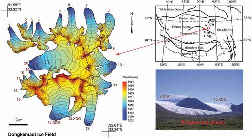
Figure 2. Comparison of (a) the reconstructed and observed daily air temperatures from 1991 to 1994 and (b) the monthly precipitation and observed from 1 July 2005 to 12 December 2008. The observed daily air temperature are from Fujita et al. (2000) and monthly precipitation is from H. Gao, He, et al. (2012)

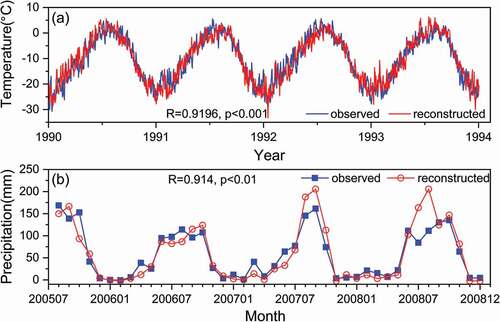
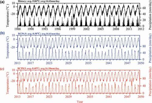
Figure 3. (a) Extrapolated daily mean air temperature and precipitation at the terminus of the XDG from 1989 to 2012 and downscaled daily mean air temperature and precipitation for (b) RCP 4.5 and (c) RCP 8.5, respectively

Data collection

The data sets used in this study include basic geographic data, field-based measurements from the XDG, meteorological data, and future climate scenarios.

Basic geographic data

The initial outlines of the individual glaciers in the DIF were downloaded from the Randolph Glacier Inventory 6.0 (https://doi.org/10.7265/N5-RGI-60), whose data for China are based on the Second Glacier Inventory of China (Guo et al. 2015). Then, the outlines were further calibrated by topographic map and aerial photographs to 1989 (Chen et al. 2017). To calibrate and parameterize the mass balance model, the initial outline of the XDG was further modified according to Pu et al. (2008) and the Landsat Thematic Mapper image of 1989, which was directly downloaded from GS Cloud of China (http://www.gscloud.cn/).

The Shuttle Radar Topography Mission version 4.1 (void filled version) digital elevation model (DEM; http://seamless.usgs.gov/), with a horizontal resolution of 30 m was used to compute average elevation, slope, aspect, latitude, and longitude for each individual glacier in the DIF. The DEM was also used as the base grid for temperature, precipitation, and snow depth interpolation and glacier surface solar radiation and shading calculation. All maps and images were created using ArcGIS 10.2 software and projected into the Universal Transverse Mercator coordinate system referenced to the 1984 World Geodetic System.

Field-based measurements in XDG

Two automatic weather stations (AWS) in the XDG, located at 5,600 and 5,216 m a.s.l., respectively, provide the basic information about the lapse rate of air temperature and precipitation gradient. Observations of annual mass balance (1989–2012), snow depth (1989–1994), and stakes data (1990–1994, 1999–2002) were carried out over the past several decades. Detailed methods for observation and data sets have been described in the literature (Fujita et al. 2000; Pu et al. 2008; Yao et al. 2012; J. Zhang et al. 2013; P. Shi et al. 2016). In this study, we used all of the above data sets collected at the XDG to calibrate and validate the mass balance model.

Meteorological station data

Four closest meteorological stations around the DIF were selected, and the daily air temperature and precipitation were collected. Detailed information on the meteorological stations is provided in Table 1. The data sets were directly downloaded from the China Meteorological Data Sharing Service System (http://data.cma.cn/). According to previous studies, climate change at the XDG has a relatively strong correlation with these four meteorological stations, especially with Tuotuohe (Pu et al. 2008; H. Gao et al. 2012; J. Zhang et al. 2013; X. Wu et al. 2015). We used these four stations to reconstruct the daily air temperature and precipitation for the glaciers in the DIF and to analyze the response of glacier mass balance to climate change.

Table 1. Ground-based meteorological data

Stations	Periods	Latitude (° N)	Longitude (° E)	Altitude (m a.s.l.)	Pannual (mm)	Psummer (mm)	Tannual (°C)	Tsummer (°C)
WDL	1957–2013	35.22	93.08	4,612	278.1	256.0	−5.37	2.94
TTH	1957–2013	34.22	92.43	4,533	280.9	259.1	−4.05	4.96
AD	1966–2013	32.35	91.10	4,800	442.2	404.5	−2.80	5.62
NQ	1955–2013	31.48	92.07	4,507	398.7	353.8	−1.28	6.85

Notes. P_annual and P_summer denote annual and summer precipitation, respectively, and T_annual and T_summer indicate annual and summer air temperatures, respectively. WDL, TTH, AD, and NQ indicate the Wudaoliang, Tuotuohe, Anduo and Naqu weather stations, respectively.

Future climate scenarios

We employed the outputs from the Regional Climate Model Version 3.0 (RegCM3) as climate forcing scenarios for our modeling period 2013 to 2050. RegCM3 is the most precise, up-to-date, and highest-resolution climate projection data for the TP (X. Gao et al. 2012; L. Zhao, Ding, and Moore 2014). The horizontal grid spacing is 25 km, and the model domain covers all of China and surrounding areas in East Asia (X. Gao et al. 2012). The model simulation extends from 1948 to 2100, a total of 153 years. The first three years are used for model spin-up, so the effective range of simulation years spans 1950 to 2100. We adopted the results of RCP 4.5 and RCP 8.5 from 2013 to 2050 (http://www.climatechange-data.cn/), in which radiative forcing is stabilized at approximately 4.5 W m⁻² and greater than 8.5 W m⁻² after 2100, respectively. Generally, RCP 4.5 represents the median scenarios for climate change in the future and the RCPs.

Methods

Glacier mass balance model description

A modified grid-based temperature index model is applied in this study. For each individual glacier, the applied glacier mass balance model can be described with the following formula (Oerlemans and Fortuin 1992):

(1) $B=\underset{t}{\int }[(1-f)\cdot M+P_s]dt$(1)

where B (m w.e.) is the glacier mass balance; f is the freezing rate of meltwater infiltration occurring in snow or firn; M (m w.e.) is the ablation water equivalent of ice and snow; P_s (mm w.e.) is the accumulation and is equal to solid precipitation; and t is the selected time period.

It was observed that in the mid- to northern TP approximately 20 percent of meltwater is preserved at the snow–ice boundary due to the refreezing process (Fujita, Ohta, and Ageta 2007), so f was assigned a value of 0.2. Ablation is calculated by applying the distributed enhanced temperature index mass balance model (Hock 1999), which elaborates on classical degree-day models by varying factors as a function of potential direct solar radiation in order to account for the effects of slope, aspect, and shading (Hock 2003). Daily temperature and precipitation are required input data, which makes the model applicable to areas with poor spatial coverage of observed weather data. Thus, daily surface ablation rates M are calculated for each grid cell of the 30-m DEM by

(2) $M=\left\{{ }_{\genfrac{}{}{0ex}{}{}{0:T\le 0{}^{\circ }C}}^{(f_M+{\alpha }_{snow/ice}{I}_{pot})\cdot T:T>0{}^{\circ }C}\right.$(2)

where ${\mathrm{f}}_{\mathrm{M}}$ (mm d⁻¹°C⁻¹) denotes a melt factor; ${\alpha }_{snow/ice}$ is a radiation factor for ice- and snow-covered surfaces; T (°C) is the air temperature, which is extrapolated from mean glacier elevation to every grid cell using a constant lapse rate from the two AWSs in the XDG; and I_pot (W m⁻²) is the potential solar radiation at the glacier surface under clear sky conditions, which can be calculated after Hock (1999):

(3) $I_{pot}=I_0\cdot {\left(\frac{R_m}{R}\right)}^2\cdot {{\mathrm{\Psi }}_a}^{\left(\frac{P}{P_{0}cosZ}\right)}\cdot \left[cos\beta cosZ+sin\beta sinZcos\left({\phi }_{sun}-{\phi }_{slope}\right)\right]$(3)

where I₀ (I₀ = 1,362 Wm⁻²) is the solar constant; (R_m/R) is the correlation factor of Earth’s orbit eccentricity; R is the instantaneous Earth–Sun distance; R_m is the average Earth–Sun distance; Ψ_a (Ψ_a = 0.75) is the mean atmospheric clear sky transmissivity (Hock 1999, 2003); P₀ (P₀ = 1,013.25 hPa) is the standard atmospheric pressure; P (hPa) is the atmospheric pressure at different latitudes; Z is the local zenith angle; β is the slope angle; φ_sun is the solar azimuth angle; and φ_slope is the slope azimuth angle.

Accumulation is assumed to be equal to solid precipitation and is calculated by using a threshold temperature method (Kang et al. 1999):

(4) $P_s=\left\{\begin{array}{c}{P}_{t}T<T_s\\ \frac{T_1-T}{T_1-T_s}{P}_t{T}_s\le T\le T_r\\ 0T>T_r\end{array}\right.$(4)

(5) $P_r=P_t-P_s$(5)

where P_s, P_r, and P_t are snow, rain, and total precipitation, respectively (mm), and T_s and T₁ are the threshold temperatures for solid and liquid precipitation, with values of 0°C and 2°C, respectively.

Climate data reconstruction and downscaling

Climate data reconstruction

Because of a lack of long-term meteorological data in the study region, we used the Tuotuohe (TTH), Wudaoliang (WDL), Anduo (AD), and Naqu (NQ) meteorological data to reconstruct the daily temperature and precipitation for the glaciers in the DIF. The daily air temperature was obtained by polynomial interpolation based on AWS data from 2005 to 2008 and four national meteorological stations (H. Gao et al. 2012). The precipitation gradient and inverse distance weighting were combined to reconstruct the daily precipitation to 5,216 m a.s.l. of the glacier surface (H. Gao et al. 2012; X. Wu et al. 2015). The detailed calculation methods are as follows:

(6) $T_0=0.473\times T_1+0.116\times T_2-0.035\times T_3+0.424\times T_4-3.149,{\mathrm{R}}^2=0.873$(6)

(7) $P_0=\frac{93}{93+173.8}\times \frac{472}{445.9}\times P_1+\frac{173.8}{93+173.8}\times \frac{472}{434.9}\times P_2$(7)

where $T_0$ (°C) and $P_0$ (mm) represent the temperature and precipitation, respectively, at 5,216 m a.s.l. in Dongkemadi River basin. $T_1$, $T_2$, $T_3$, and $T_4$ (°C) are air temperatures recorded at TTH, WDL, AD, and NQ meteorological stations, and $P_1$ and$P_2$ (mm) denote precipitation recorded at AD and NQ, respectively.

As shown in Figure 2, the reconstructed daily temperature is in good agreement with observations (R² = 0.9196, p < .001). However, the reconstructed daily precipitation is far from satisfactory, with R² < 0.4, but the monthly comparison between the reconstructed and observed is R² = 0.91. The reasons for this are discussed in detail by H. Gao et al. (2012).

Future scenarios downscaling

High-resolution climate forcing downscaling from the RegCM3 to the terminus of each individual glacier in the DIF is a crucial step in projecting the glacier variation under the future climate scenarios. Here, we applied RCP 4.5 and RCP 8.5 scenarios for our modeling period 2013 to 2050. The overall downscaling method is as follows: First, we extracted RegCM3 projected temperatures and precipitation from the nearest four gridpoints around each individual meteorological station (WDL, TTH, AD, and NQ) and then applied a bilinear interpolation method to produce the raw climate data. Second, the raw data were corrected based on data from the meteorological stations for the period 1989 to 2012 using a local scaling method (Salathé 2005). Daily precipitation was downscaled as follows:

(8) $P_{ds}(x,t)=P_{\mathrm{m}\mathrm{o}\mathrm{d}}(x,t)\frac{{(P_{obs})}_{sea}}{{(P_{\mathrm{m}\mathrm{o}\mathrm{d}})}_{sea}}$(8)

where P_mod(x,t) is the RegCM3 simulated monthly mean precipitation (mm) for the gridpoint containing a location x and at time t in season “sea”; (P_obs)_sea and (P_mod)_sea refer to the seasonal mean taken over the fitting period (the overlap of the observed data set at meteorological stations and the historic run extracted from RegCM3). The air temperature is downscaled in a way similar to that for precipitation. For temperature, the adjustment is additive (Salathé 2005); thus, the downscaled daily air temperature is given by

(9) $T_{ds}(x,t)=T_{\mathrm{m}\mathrm{o}\mathrm{d}}(x,t)+[(T_{obs}{)}_{sea}-(T_{\mathrm{m}\mathrm{o}\mathrm{d}}{)}_{sea}]$(9)

where T_mod(x,t) is the RegCM3 simulated monthly mean temperature (°C) for the gridpoint at location x and at time t in season “sea”; (T_obs)_sea and (T_mod)_sea is the seasonal mean taken over the fitting period (1989–2012).

Third, applying Equations (6(6) $T_0=0.473\times T_1+0.116\times T_2-0.035\times T_3+0.424\times T_4-3.149,{\mathrm{R}}^2=0.873$(6) ) and (7(7) $P_0=\frac{93}{93+173.8}\times \frac{472}{445.9}\times P_1+\frac{173.8}{93+173.8}\times \frac{472}{434.9}\times P_2$(7) ), we generated a time series of daily temperature and precipitation for each glacier in the DIF from 2013 to 2050. The reconstructed historical climate data and the downscaled projection data at the XDG are shown in Figure 3.

Area, volume, and terminus elevation estimation

Because ice thickness data for ice flow modeling were not available, we used a modified V-A scaling method (Marzeion, Jarosch, and Hofer 2012) to estimate the area, volume, and terminus elevation changes for each individual glacier in the DIF from 1989 to 2050.

Glacier area and volume

After Radić, Hock, and Oerlemans (2008) and Marzeion, Jarosch, and Hofer (2012), volume (V) and area (A) of a single glacier at the start year are

(10) $V_0=c_a(A_0{)}^{\mathrm{{\rm Y}}}$(10)

where A₀ (km²) is the surface area of the glacier in 1989, which was calculated from the outlines using ArcGIS; c_a is equal to 0.2055 m (3 − 2γ); and γ is equal to 1.375. These coefficients are provided by Radić, Hock, and Oerlemans (2008) and have been successfully applied in mountain glacier studies of the TP (Radić and Hock 2010; Radić et al. 2014; P. Shi et al. 2016). The volume change dV (km³) and dA (km²) of the glacier for each mass balance period (from October to September) is further determined by the method of Marzeion, Jarosch, and Hofer (2012) as

(11) $dV(n+1)=1/\rho \cdot A(n)\cdot B(n)$(11)

(12) $dA(n+1)=\frac{1}{{\tau }_A}\left({\left(\frac{V(n+1)}{c{\hspace{0.17em}}_a}\right)}^{1/\gamma }-A(n)\right)$(12)

where A(n) and B(n) (m w.e.) are the glacier area and glacier mass balance in the nth year (see Equation 1(1) $B=\underset{t}{\int }[(1-f)\cdot M+P_s]dt$(1) ), respectively, and ρ (ρ = 900 kg m⁻³) is the ice density. τ_A is a relaxation time series scale and is calculated as

(13) ${\tau }_A(n)={\tau }_L(n)\frac{A(n)}{L{(n)}^2}$(13)

where L(n) and τ_L are glacier length and the response timescale of glacier length in the nth year, respectively. The glacier length in the start year is estimated following the method of Marzeion, Jarosch, and Hofer (2012) as

(14) $L_0=c_L\cdot (A_0{)}^q$(14)

where q and c_L are scaling parameters and are taken from literature as q = 2.2 (Bahr, Pfeffer, and Kaser 2015) and c_L = 0.0180 km^3−q (Radić et al. 2014) for glaciers. During the model integration, length changes dL (km) for each mass balance period are estimated as

(15) $dL(n+1)=\frac{1}{{\tau }_L}\left({\left(\frac{V\left(n+1\right)}{c_L}\right)}^{1/q}-L(n)\right)$(15)

where L(t) is the glacier’s length at the start of the mass balance year, and τ_L is a relaxation timescale and can be estimated as

(16) ${\tau }_L(n)=\frac{V(n)}{A(n){P_r}_s(n)}$(16)

Terminus elevation change

We applied the approach originally developed by Marzeion, Jarosch, and Hofer (2012) and further modified by L. Zhao et al. (2017) to calculate the terminus elevation change. Before calculation, we assumed a linear increase of the terminus elevation Z_min (m) with decreasing glacier length L (km). For retreating glaciers, we directly removed grid cells near the glacier terminus from the glacier surface grids and obtained a new glacier terminus position and hence a new outline for the next year. For advancing glaciers, we added gridpoints to the glacier surface grid, whose elevations were supposed to be the glacier elevation minimum in the n + 1st year, z_min (n + 1), which was obtained as follows by assuming a constant glacier surface slope:

(17) $z_{min}(n+1)=z_{max}(n+1)+\frac{L(n+1)}{L(n)}\cdot \left(z_{min}(n)-z_{max}(n)\right)$(17)

where z_max(n + 1) denotes the glacier’s maximum elevation in the n + 1st year, which is determined by finding the Shuttle Radar Topography Mission DEM maximum elevation within an individual glacier outline. It is held constant during the modeling process. L(n + 1) is the n + 1st year glacier length, and L(n) is the length of the glacier in the year of the surface area measurement.

Results

Parameters calibration and results validation

We used the years 2008 to 2012 to calibrate the mass balance model and 1989 to 2007 to validate the model performance. An overall sketch map of the modeling process is shown in Figure 4a. For calibration, we used a constant lapse rate λT (λT = 0.63°C/100 m) and λP (λP = 30 percent/100 m), both calculated from two AWS in the XDG (Fujita et al. 2000; Pu et al. 2008), to extrapolate air temperature and precipitation to cell grids for each individual glacier. In addition to these two parameters, the melt factor f_m and the radiation coefficient α_ice/snow need to be determined. In this study, a Monte Carlo method was used with a total of 100 runs to yield the minimum root mean square deviation between the measured and modeled mass balance in the XDG (Figure 4c). Detailed information on the parameters used in the model is provided in Table 2.

Table 2. Applied parameters of the model optimized for all measured mass balance series in the DIF

Parameter	Value	Unit
Temperature lapse rate, λT	0.63	°C/(100 m)
Melt factor, fm	4	mm day^−1°C^−1
Radiation coefficient for snow, αsnow	7.5	mm day^−1 W^−1 m^2°C^−1
Radiation coefficient for ice,αice	15	mm day^−1 W^−1 m^2°C^−1
Precipitation gradient, λP	30	%/100 m
Precipitation correction factor, S	25	%

Figure 4. Comparison between simulated and measured (a) annual mass balance and (b) ELA and (c) scatterplot of calculated vs. measured mass balance at individual stakes on the XDG. The vertical bar denotes the 1δ standard deviation

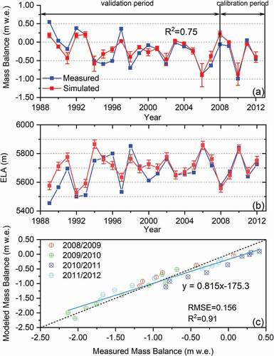
Figure 4a illustrates a comparison between the observed and modeled mass balance in the XDG. The simulated mean annual mass balance during 1989 to 2012 was −0.233 m w.e., which is close to the value of −0.213 m w.e. observed for the XDG. To further evaluate the performance of the mass balance model, the coefficient of determination (R²), Nash-Sutcliffe efficiency, and root mean square error were determined. The simulated and observed R² was 0.75 from 1989 to 2012, whereas the value was higher and reached 0.90 during the period 2001 to 2002. In addition, the Nash-Sutcliffe efficiency and root mean square error reached 0.77 and 0.156, respectively, during the whole modeling period. Thus, the simulated results fit well with the observations, especially after 2001. Additionally, the ELA is a theoretical line on a glacier at which annual mass accumulation equals mass loss. In this study, the simulated ELA also had a higher correlation with observations from 2001 to 2012 (R² = 0.90, p < .001; Figure 4b), further suggesting that the model can reproduce glacier mass balance change reasonably well. Considering that the climatic regimes are nearly the same among the glaciers in the DIF, we directly extended this model to the whole DIF to estimate the mass balance change by using the parameters obtained from the XDG.

Mass balance variation in DIF from 1989 to 2050

Sixty-two years of annual mass balance, ablation, and accumulation for all glaciers in the DIF were obtained by employing the distributed enhanced temperature index model. We adopted the method used by Chen et al. (2017) to calculate the mass balance (B_total) for the whole DIF. Figure 5 illustrates the model reconstructed and projected glacier mass balance series in DIF from 1989 to 2050. Unlike the previous studies that suggested that the annual mass balance at XDG was positive between 1989 and 1993 and negative for most years since 1994 (Fujita et al. 2000; Pu et al. 2008; J. Zhang et al. 2013), the reconstructed mass balance on the whole DIF shows a continuously negative trend with a linear rate of −0.08 m w.e. year⁻¹ from 1989 to 2012. The cumulative mass loss was about 12.58 m w.e. (Figures 6 and Figure 7); thus, the DIF has thinned about 13.98 m (assuming a glacier density of 0.9 g cm⁻³).

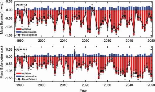
In the future, the mass balance will remain negative for most years under RCP 4.5. Despite several positive years, such as 2023, the negative trend will remain continuous with a linear rate of −0.16 m w.e. a⁻¹. At the end of 2050, the DIF will have lost 37.48 m w.e., equivalent to thinning of 41.64 m. Similarly, the mass balance shows a significantly negative trend with a rate of −0.35 m w.e. a⁻¹ in RCP 8.5. There are also positive years under RCP 8.5, such as 2015 (0.46 m w.e). At the end of 2050, the DIF will have lost 43.01 m w.e. in RCP 8.5, corresponding to thinning of 47.79 m. In short, the mass balance of the DIF will maintain a generally negative trend under both RCP 4.5 and RCP 8.5. Additionally, based on the ablation and accumulation in a mass balance year (Figure 5), the mean annual mass gain for the DIF is about 0.099 m w.e. a⁻¹ for the period 1989 to 2012, 0.166 m w.e. a⁻¹ for RCP 4.5 and 0.142 m w.e. a⁻¹ for RCP 8.5. However, the average annual mass loss for the DIF was about −0.596 m w.e. a⁻¹ for 1989 to 2012 and will reach −0.826 m w.e. a⁻¹ for RCP4.5 and −0.943 m w.e. a⁻¹ for RCP 8.5. It is clear that the mass gain is significantly lower than the mass loss. The climate condition shift (Ke et al. 2017) and local air temperature rise (Pu et al. 2008; L. Zhao, Ding, and Moore 2014) may both cause glacier mass loss in the DIF.

Figure 5. Seasonal variation in mass balance in the DIF during the period 1989 to 2050 under RCP 4.5 and RCP 8.5. The blue and red bars denote accumulation and ablation, respectively, and the black samples and line refer to the annual net mass balance. Error bar indicates the standard deviation of the results

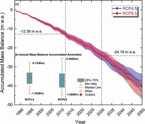
Table 3 shows the simulated results compared with previous geodetic studies (Chen et al. 2017). The simulated annual mean mass balance in the XDG is close to the glaciological and geodetic results, but the simulated mass balance in the DIF seems lower than the geodetic results. The primary reason for this is that the area of DIF in the previous study is only 73.6 km² (Chen et al. 2017), but the area in our study is about 83.9 km². Glacier-wide mass balance is highly correlated to the glacier area. If we adjust the initial area to 73.6 km², the mean annual mass balance is about 0.83 m w.e., which is much closer to the geodetic results. However, from a previous study conducted by Z. Li et al. (2012), an area of 83.9 km² represents the real area of the DIF in 1989. In addition, as Figure 6 shows, the accumulated mass loss will undergo two large shifts from 1989 to 2050. Before 2012, the rate of accumulated mass loss was only −0.45 m w.e. a⁻¹; however, it will reach −0.59 m w.e. a⁻¹ during the period 2013 to 2030 in both RCP 4.5 or RCP 8.5. After 2030, the rate will dramatically increase to −0.68 m w.e. a⁻¹ in RCP 4.5 and −1.02 m w.e. a⁻¹ in RCP 8.5. If the mass balance keeps decreasing at an accumulated rate of −0.52 ± 0.004 m w.e. a⁻¹ (1989–2050), the DIF will decrease by at least 66.5 ± 2.5 m w.e. at the end of the twenty-first century, corresponding to thinning of at least 73.89 m. However, according to field observations conducted by Z. Wu et al. (2018), the maximum thickness of the XDG is only 109 m. Therefore, it can be concluded that most of the glaciers in the DIF will melt by the end of 2100.

Table 3. The annual mean mass balance of the XDG and DIF during different periods

	Glaciological results^a	Geodetic results^b		Simulated results^c
Period	XDG (m w.e. year^−1)	XDG (m w.e. year^−1)	DIF (m w.e. year^−1)	XDG (m w.e. year^−1)	DIF (m w.e. year^−1)
1969–1999	—	−0.06 ± 0.10	–0.21 ± 0.10	—	—
1989–1999	−0.12	—	—	−0.14	−0.46
1999–2015	−0.42	−0.41 ± 0.21	–0.74 ± 0.21	−0.39 ± 0.01	−0.56 ± 0.01
2015–2050	—	—	—	−0.63 ± 0.07	−0.72 ± 0.07
1989–2050	—	—	—	−0.48 ± 0.05	−0.64 ± 0.05

Notes. ^aData from Pu et al. (2007).

^bData from Chen et al. (2017).

^cThis study.

Figure 6. (a) Accumulated mass balance during 1989 to 2050 and (b) anomalies in accumulated annual mass balance

Mass balance gradient on the DIF

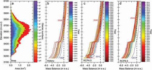
Mass balance is most sensitive to climate change with elevation. Here, we further reconstructed mass balance variation vs. the elevation on the DIF from 1989 to 2050. As Figures 7b and Figure 7c show, the mass balance gradient of each year exhibits an increasing trend along with elevation rise. The area–altitude distribution clearly reveals that the ELA fluctuates around the altitude at which the glacier has the maximum area (Figure 7a). This pattern is also in line with the general understanding of mountain glaciers (Yao et al. 2012) and is supported by recent studies conducted in the XDG (J. Zhang et al. 2013; P. Shi et al. 2016; Z. Zhang et al. 2018). For the DIF, the ELA fluctuates between 5,560 and 5,945 m a.s.l. for most individual glaciers during the period 1989 to 2012. Previous studies have reported that the ELA varied from 5,600 to 5,840 m a.s.l. from 1990 to 2008 in the XDG (Pu et al. 2008; J. Zhang et al. 2013). However, the ELA will reach 5,570 to 5,850 m a.s.l. for most individual glaciers in the DIF under RCP 4.5 and will reach 5,640 to 5,900 m a.s.l. in RCP 8.5. To summarize, the average ELA in the DIF is 5,650 m a.s.l. for the period 1989 to 2012, and it will reach 5,800 m a.s.l. in RCP 4.5 and 5,850 m a.s.l. in RCP 8.5. After 2030, the average altitude of the ELA in the DIF will be much higher than 5,800 m a.s.l., which is higher than the summit of several glaciers in the southern part of the DIF. Therefore, it can be concluded that the whole DIF will experience a dramatic shrinkage after 2030. In addition, although the minimum ELA was found in 2015 under RCP 8.5, the minimum gradient was found in 1992 with a value of −0.07 m w.e. (100 m)⁻¹. This pattern was directly related to the annual mass balance variation in 1991/1992 for a higher accumulation and lower ablation (Figure 5). In situ observations also support this result (Pu et al. 2008; J. Zhang et al. 2013). The mass balance was positive and the glacier was advanced at the XDG at the end of the 1980s and before the mid-1990s and then the mass balance became negative (Pu et al. 2008; Yao et al. 2012; P. Shi et al. 2016). Several studies attribute this to a shift in climate conditions from the 1980s to 1990s (Ke et al. 2017) and road construction adjacent to the DIF exposing the glacier surface to increased dust cover (J. Zhang et al. 2013).

Figure 7. (a) Distribution of area and (b) mass balance from 1989 to 2012 in (c) RCP 4.5 and (d) RCP 8.5 with respect to altitude in the DIF

Discussion

The area and volume variation

A continuous negative mass balance will lead to area and volume loss. However, there is a lag in the response of glacier area, volume, and terminus variation to climate change, which depends on the glacier type, size, thickness, and so on (Yao et al. 2004; Pan et al. 2012; Tian, Yang, and Liu 2014). In our study, individual glaciers in the DIF are of different types, sizes, and thicknesses, so we used the τ_A relaxation time series for area change and τ_L relaxation time series for calculation of the variation in terminus (Equations 13(13) ${\tau }_A(n)={\tau }_L(n)\frac{A(n)}{L{(n)}^2}$(13) and 16(16) ${\tau }_L(n)=\frac{V(n)}{A(n){P_r}_s(n)}$(16) ). Earlier studies have suggested that the area of glaciers in the DIF has reduced since the 1990s (Z. Li et al. 2012; Ke et al. 2017). Observations conducted in the XDG also revealed that the glacier area has shrunk since 1994/1995 (Yao et al. 2012; J. Zhang et al. 2013). In this study, area reduction was also found for all individual glaciers in DIF beginning around 1990/89, which is significantly earlier than the observation in the XDG, indicating the whole DIF may be more sensitive to climate change than previously believed.

For the DG, the area reduced 0.53 km² from 1989 to 2012 (equivalent to −0.0218 km² a⁻¹ or about 3.2 percent total loss), and the linear rate of annual reduction was −0.13 percent a⁻¹, which is close to the rate of −0.11 percent a⁻¹ (total 4.3 percent area loss from 1969 to 2019) reported in a recently published paper (Liang et al. 2019). The Second Glacier Inventory of China data set (Guo et al. 2015), based on a compilation of Landsat Thematic Mapper and Enhanced Thematic Mapper Plus images from 2006 to 2010, also showed that the area of the DG has decreased by 3.8 percent relative to 1969 (−0.10 percent a⁻¹), which was close to our estimation of about −0.13 percent a⁻¹. Z. Li et al. (2012) also indicated that the DG decreased at a linear rate of −0.0152 km² a⁻¹ from 1969 to 2000, which is somewhat lower than our rate of −0.0218 km² a⁻¹. However, if we consider that the climate condition has shifted since the 1990s (Ke et al. 2017) and the air temperature has risen since 1995, the rate of area decrease based on our calculation appears reasonable. In addition, the area of the XDG will be 1.452 km² in RCP 4.5 and 1.405 km² in RCP 8.5 at the end of 2050. Compared with an area of 1.767 km² in 1989 (adjusted after Pu et al. 2008), the XDG will lose 27 to 30 percent of its area, which is close to a 25 percent loss from 2007 to 2047 simulated by an ice flow model (Z. Wu et al. 2018).

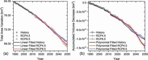
For the DIF, the area was about 83.9 km² in 1989 (adjusted after Z. Li et al. 2012), whereas the area was 76.339 km² in 2012. A, or total of −7.573 km² area loss at a rate of −0.316 km² a⁻¹, which is close to the linear rate of −0.31 ± 0.04 km²·a⁻¹ from 1969 to 2013 based on remote sensing data (Ke et al. 2017). However, this value is clearly higher than the decrease rate of −0.0677 km²·a⁻¹ calculated by Z. Li et al. (2012) using geodetic data from 1969 to 2000. This might indicate that glacier decrease dramatically increased after 2000. In fact, our calculation and Ke et al. (2017) both suggest the area loss rate is higher at 0.36 km²·a⁻¹ since 2000. As Figure 8 shows, at the end of 2050, the area of each individual glacier will have decreased 12.1 to 30.66 percent under RCP4.5 and 14.06 to 38.76 percent under RCP 8.5. This corresponds to a total area reduction in the DIF of 15.28 km² in RCP 4.5 and 16.86 km² in RCP 8.5 (Figure 9a). The whole DIF will lose about 18.21 percent of its area in RCP 4.5 and 20.09 percent in RCP 8.5. In addition, the volume of the DIF will decrease about 1.18 km³ in RCP 4.5 and 1.44 km³ in RCP 8.5 by the end of 2050. During the period 1989 to 2050 DIF will release at least about 1.179 ± 0.117 km³ runoff due to glacier melt.

The extent of glacier decrease in our study is significantly lower than that predicted by studies conducted in the Himalayan Mountains, which conclude that most glaciers will disappear entirely by 2035 if the Earth keeps warming at the current rate or will decrease at least 63 to 87 percent by the middle of the century in comparison to the glacier extent in 2005 in RCP 4.5 and RCP 8.5 (L. Li et al. 2019). Our results are also lower than those of studies that concluded that the total glacier area will decrease by 22 or 35 percent in High Mountain Asia by 2050 (L. Zhao, Ding, and Moore 2014). However, our results are higher than the projected 12 percent reduction of glaciers in western China with an air temperature rise of 1.3°C (Y. Shi and Liu 2000), close to the 11 to 18 percent losses in Qiangtang No. 1 Glacier under the historical warming trend of 0.035°C a^–1 and the A1B scenario (Y. Li et al. 2017). The Intergovernmental Panel on Climate Change fifth assessment report (2013) also projects that glaciers worldwide will lose about 15 to 85 percent under different climate scenarios by the end of the twenty-first century. If only taking into account the area loss of individual glaciers in the DIF (Figure 8), the loss of several glaciers will reach 30.66 to 38.76 percent (Figure 8), which is much closer to the average decrease in the TP (L. Zhao, Ding, and Moore 2014). Moreover, because several glaciers in the western Himalayas (H. Zhao et al. 2016) and the Karakoram (Forsythe et al. 2017) continue to expand, the extent of reduction in the DIF appears reasonable. This pattern of glacier extent reduction is in agreement with conclusions that retreat is the smallest in the TP interior and gradually increases toward the edges (Yao et al. 2012; M. Yang et al. 2019). Therefore, it is reasonable to believe that this study reflects the true state of variation in the DIF. Differences in extent of reduction for each individual glacier in the DIF also indicate that spatial heterogeneity generally exists, even in the same climate regime and in the same ice cap. The response of glaciers to climate change is a complex process that is not only affected by climate change (Mölg, Maussion, and Scherer 2014) but is also controlled by the scale, hypsometry, and orientations of the glacier itself. Sublimation and other wind-driven ablation processes also contribute to the extent of glacier variation (Litt et al. 2019), although they are beyond the scope of this study.

Figure 8. Variation in each individual glacier in the DIF from 1989 through future scenarios for 2050

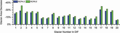
Figure 9. (a) Total area decrease and (b) volume of accumulated loss from 1989 to 2050 in the DIF. The shaded area indicates the 1δ deviation in the data

Terminus elevation variation

In comparison to the mass balance observations conducted in the DG (Pu et al. 2008; Yao et al. 2012), little work has been done on the variation in terminus elevation in the DG and other glaciers in the DIF. Field photographs provide some clues about the terminus change (Pu et al. 2008; P. Shi et al. 2016). Previous studies indicated that the terminuses of the XDG and DDG were linked together before 2000 (Fujita et al. 2000) and then were completely separated from each other by 2007 and further expanded since 2009 (Fujita, Ohta, and Ageta 2007; Pu et al. 2008). In recent years, the distance between the DDG and XDG terminuses has dramatically increased (Z. Li et al. 2012; J. Zhang et al. 2013) and the altitude of the XDG terminus rose quickly with rising air temperature (Pu et al. 2008; Yao et al. 2012; J. Zhang et al. 2013). We applied a modified method originally developed by Marzeion, Jarosch, and Hofer (2012) to reconstruct and project the variation in terminus elevation for each individual glacier in the DIF. The simulated results show that the terminuses of the DDG and XDG were linked during 1989/1990 (Figure 10a), and they were still linked until 2004/2005, although several parts of the terminus had begun to melt and the altitude rose. Since then, the DDG and XDG were gradually separated from each other and were completely separated by 2007/2008. Figure 10b shows the terminus altitude of the XDG. The altitude rose from 5,380 m a.s.l. in 1990/1989 to 5,454 m a.s.l. in 2012/2011, and observations at the XDG suggested that the terminus was located at 5,380 m a.s.l. in 1994/1995 and rose to 5,420 m a.s.l. in 2012/2011 (J. Zhang et al. 2013). If the XDG mass balance, which was positive before 1994 (Fujita et al. 2000; Pu et al. 2008; Yao et al. 2012), had not changed over time, the terminus would have advanced or at least remained at 5,380 m a.s.l. therefore, our simulated results are close to the observations from 1989 to 2012.

Figure 10. Spatial variation in mass balance and terminus elevation of the (a) DDG and (b) XDG from 1989 to 2012. The black lines show the glacier boundaries in 1989 and the red numbers are the altitudes of the glacier terminus in the respective years

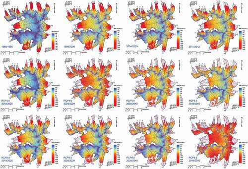
For the whole DIF, the changes in terminus altitude show an apparent relationship between glacier melt and orientation. As shown in Figure 11, the terminuses rose quickly in the northern part of the DIF but relatively slowly in the south, west, and east. This pattern is in agreement with observations that the terminus altitudes are generally higher in the northern parts than in the southern parts of mountains I the TP (Yao et al. 2012; M. Yang et al. 2019). In 1989, the terminuses of most of the glaciers in the northern part of the DIF were located at 5,300 m a.s.l.; however, they will reach ~5,500 m a.s.l. in RCP 4.5 and ~5,600 m a.s.l. in RCP 8.5. In contrast, the terminus altitudes of most glaciers in the DIF facing other directions were located at 5,250 m a.s.l. in 1989. At the end of 2050, the terminus elevations of these glaciers will rise to ~5,520 m a.s.l. in RCP 4.5 and ~5,570 m a.s.l. in RCP 8.5. Additionally, it should be noted that the middle of the DDG melts quickly, which may lead to an earlier disappearance in the middle than in other parts of the terminus. This melting pattern in the DDG waas also observed by Z. Li et al. (2012), suggesting that the DDG shows obvious thinning in the middle parts, wheras the upper part and the terminus might be slight thickening. From our simulation and from previous remote sensing studies (Z. Li et al. 2012), the DDG will be separated into two glaciers in the future, which also implies that the maximum glacier melt occurs not only at the terminus (glacier front) but also in the other parts. The same phenomenon is also seen in Glacier No. 7 in the northern part of the DIF.

In Figures 10 and Figure 11, we overlay the spatial variation of mass balance to the variation in terminus elevation, demonstrating the variation in accumulation and ablation areas as well as ELA fluctuations. From 1989 to 2012, the ablation area dramatically increased and the accumulation area accordingly decreased. In the future, although the accumulation area will increase because of positive mass balance in several years, the ablation area will increase at an accelerated rate in most years, especially after the 2030s. From this perspective, the variation in glaciers will undergo three distinct stages: an initial gradual melt stage, followed by a relatively quick melt stage, and finally a fast melt stage. At the end of 2050, accumulation can only be found in limited high elevation areas in RCP 4.5 but not in RCP 8.5. This model result further confirms the assumption that the DIF will continue to lose area and volume in future scenarios.

Figure 11. Spatial variation in mass balance and terminus elevation for all glaciers in the DIF from 1989 to 2050. The black lines show the glacier boundaries in 1989

Glacier mass balance response to air temperature and precipitation change

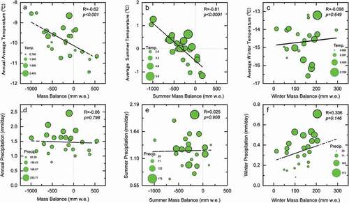
Glacier variation is dominated by ablation and accumulation processes. Warmer annual air temperatures cause glaciers to melt, but the increased annual precipitation generally leads to mass accumulation (Y. Wang et al. 2008). Because glacier mass balance has a direct relationship between glacier variation and climate change (Bolch et al. 2012), we analyzed the relationship between temperature, precipitation, and mass balance. As Figure 12 shows, air temperature has a clear negative correlation with the annual variation in mass balance (R² = −0.61, p < .001), particularly in the summer (R² = −0.81, p < .001), indicating that air temperature has a greater effect on mass balance than precipitation. Because the annual mass balance has a higher correlation with the summer mass balance (R² = 0.96, p < .001) than with the winter mass balance (R² = 0.05, p < .01), the long-term variation in mass balance is mainly controlled by summer mass balance, despite considerable year-to-year variability in winter mass balance. Thus, it can be reasonably concluded that the mass balance in the DIF is strongly controlled by the summer air temperature variation. Previous studies have also suggested that though the annual air temperature rises at a rate of 0.06°C a⁻¹, the annual summer air temperature has increased at a rate of 0.08°C a⁻¹ since 1989 in this area (Pu et al. 2008; Z. Li et al. 2012; P. Shi et al. 2016). This is much higher than the average summer rate of 0.067°C a⁻¹ observed since 2000 in the TP (Kuang and Jiao 2016). In short, rising air temperature causes a negative mass balance and glacier melt in the DIF.

On the other hand, precipitation has a high positive correlation with winter mass balance (Figure 12f), indicating that precipitation mainly influences winter mass balance but not summer mass balance. However, for the long-term variation in mass balance, annual and summer precipitation appear to play a limited role in variation in mass balance (Figure 12d), because ablation and accumulation both occur during summer in the DIF (Pu et al. 2008; Z. Zhang et al. 2018). Previous studies have suggested that since the 1990s annual precipitation has slightly increased at a linear rate of 0.03 mm a⁻¹ and summer precipitation has increased at a rate of 0.08 mm a⁻¹ since the 1990s (Pu et al. 2008; P. Shi et al. 2016); however, the increasing rate of precipitation is relatively lower than that of air temperature. Oerlemans (2005) pointed out that the effect of a 1 °C warming on glacier mass balance is equivalent to that of a 25 percent increase in precipitation. In addition, though precipitation has increased at a low rate since 1989, total precipitation in the 1990s decreased by 15.6 mm compared to that in the 1980s in the region (Z. Li et al. 2012). Therefore, the mass balance was negative in most years since the 1990s. Thus, the rise of air temperature, particularly in the summer season, mainly controls the variation in the DIF.

Figure 12. Correlation between mass balance and means (annual, summer, and winter air temperatures) or total (annual, summer, and winter precipitation) local climate forcing from simple linear regression analysis for 1989 to 2012 in the XDG. Dashed lines represent changing trends with indicators. The summer season corresponds to the months June to September

In addition, although the combined effects of air temperature and precipitation are predominant (Z. Li et al. 2010; Yao et al. 2012), they are closely associated with large or regional-scale atmospheric circulation, such as North Atlantic Oscillation, Southern Oscillation Index, Indian Monsoon, East Asian Summer Monsoon, and others (Forsythe et al. 2017; Mölg, Maussion, and Scherer 2014; W. Yang, Guo, et al. 2016), which directly cause changes in regional air temperature and precipitation (Pu et al. 2008; Z. Zhang et al. 2018) and were responsible for shifts in climate patterns that occurred in 1989/1990 (Ke et al. 2017). Therefore, large-scale variation in circulation affects regional climate change and results in variations in the glaciers in the DIF.

Conclusions

To obtain the variation in mass balance for the whole DIF and to project its future variation under RCP 4.5 and RCP 8.5, an enhanced distributed mass balance model coupled with a modified V-A scaling method was applied in this study. The advantage of the adopted method is that it can effectively reduce the error produced by the glacier area change and substantially improve the accuracy of area and volume projections, especially for the low altitude area of the glacier. The modeled XDG mass balance was in good agreement with observations conducted in the XDG from 1989 to 2012. The performance of ELA simulation was improved, with reproduction of the variation in the XDG. With reconstructed daily air temperature and precipitation from four adjacent meteorological stations, the mass balance of the DIF showed a continuously negative trend with a mean annual rate of −0.16 m w.e. a⁻¹ in RCP 4.5 and −0.35 m w.e. a⁻¹ in RCP 8.5 (2013–2050). Both rates were higher than the rate of −0.08 m w.e. a⁻¹ from 1989 to 2012, indicating that glacier loss will accelerate in the future climate scenarios. If the glacier continues to thin at a mean annual accumulative rate of −0.52 ± 0.004 m w.e. a⁻¹, most glaciers in the DIF will melt by the end of the twenty-first century.

The area reduction of individual glaciers in the DIF varies widely. From 1989 to 2050, each individual glacier in the DIF will lose 12.10 to 30.66 percent under RCP 4.5 and 14.06 to 38.76 percent under RCP 8.5, and the total area of the DIF will be reduced about 15.28 km² in RCP 4.5 and 16.86 km² in RCP 8.5. Obvious differences in the extent of reduction for each individual glacier in the DIF also indicate spatial heterogeneity overall, even in the same climate regime and in the same ice cap. Overall, the DIF will lose about 18.21 percent of its area in RCP 4.5 and 20.09 percent in RCP 8.5, equivalent to a loss of about 1.18 km³ in RCP 4.5 and 1.44 km³ in RCP 8.5 by the end of 2050. Simultaneously, mountain runoff due to glacier melt will reach at least 1.179 ± 0.117 km³. Additionally, the terminuses of individual glaciers will undergo a dramatic rise and most glacier terminuses will reach ~5,520 m a.s.l. in RCP 4.5 and ~5,570 m a.s.l. in RCP 8.5, which is close to the XDG average ELA in 1989. The clearly increasing summer air temperature and relatively stable precipitation seem to be the main reasons for glacier shrinkage in the DIF. If the warming trend continues as projected in RCP 4.5 or RCP 8.5, most of the DIF will have melted by the end of the twenty-first century.

Acknowledgments

We acknowledge the Chinese National Climate Center for providing data from their regional climate simulation models.

Disclosure Statement

No potential conflict of interest was reported by the authors.

Additional information

Funding

This research is supported by the China Postdoctoral Science Foundation (Nos. 2017M610622, 2017BSHEDZZ18), the Natural Science Foundation of Shaanxi Province, China (No. 2018JM4008), National Natural Science Foundation of China (Nos. 41571062, 41771030), and Fundamental Research Funds for the Central Universities of Shaanxi Normal University (Nos. GK201703051 and GK201803047).

References

- Bahr, D. B., W. T. Pfeffer, and G. Kaser. 2015. A review of volume-area scaling of glaciers. Reviews of Geophysics 53 (1):95–140. doi:https://doi.org/10.1002/2014RG000470.
- Bliss, A., R. Hock, and V. Radić. 2014. Global response of glacier runoff to twenty-first century climate change. Journal of Geophysical Research: Earth Surface 119 (4):2013J–2931J.
- Bolch, T., A. Kulkarni, A. Kaab, C. Huggel, F. Paul, J. G. Cogley, H. Frey, J. S. Kargel, K. Fujita, M. Scheel, et al. 2012. The state and fate of Himalayan glaciers. Science 336 (6079):310–14. doi:https://doi.org/10.1126/science.1215828.
- Bonanno, R., C. Ronchi, B. Cagnazzi, and A. Provenzale. 2014. Glacier response to current climate change and future scenarios in the northwestern Italian Alps. Regional Environmental Change 14 (2):633–43. doi:https://doi.org/10.1007/s10113-013-0523-6.
- Chen, A., N. Wang, Z. Li, Y. Wu, W. Zhang, and Z. Guo. 2017. Region-wide glacier mass budgets for the Tanggula Mountains between ~1969 and ~2015 derived from remote sensing data. Arctic, Antarctic, and Alpine Research 49 (4):551–68. doi:https://doi.org/10.1657/AAAR0016-065.
- Forsythe, N., H. J. Fowler, X. Li, S. Blenkinsop, and D. Pritchard. 2017. Karakoram temperature and glacial melt driven by regional atmospheric circulation variability. Nature Climate Change 7 (9):664–70. doi:https://doi.org/10.1038/nclimate3361.
- Fujita, K. 2008. Effect of precipitation seasonality on climatic sensitivity of glacier mass balance. Earth and Planetary Science Letters 276 (1–2):14–19. doi:https://doi.org/10.1016/j.epsl.2008.08.028.
- Fujita, K., and T. Nuimura. 2011. Spatially heterogeneous wastage of Himalayan glaciers. Proceedings of the National Academy of Sciences of the United States of America 108 (34):14011–14. doi:https://doi.org/10.1073/pnas.1106242108.
- Fujita, K., T. Ohta, and Y. Ageta. 2007. Characteristics and climatic sensitivities of runoff from a cold-type glacier on the Tibetan Plateau. Hydrological Processes 21 (21):2882–91. doi:https://doi.org/10.1002/()1099-1085.
- Fujita, K., Y. Ageta, P. Jianchen, and Y. Tandong. 2000. Mass balance of Xiao Dongkemadi glacier on the central Tibetan Plateau from 1989 to 1995. Annals of Glaciology 31 (1):159–63. doi:https://doi.org/10.3189/172756400781820075.
- Gabbi, J., M. Carenzo, F. Pellicciotti, A. Bauder, and M. Funk. 2014. A comparison of empirical and physically based glacier surface melt models for long-term simulations of glacier response. Journal of Glaciology 60 (224):1140–54. doi:https://doi.org/10.3189/2014JoG14J011.
- Gao, H., X. He, B. Ye, and J. Pu. 2012. Modeling the runoff and glacier mass balance in a small watershed on the Central Tibetan Plateau, China, from 1955 to 2008. Hydrological Processes 26 (11):1593–603. doi:https://doi.org/10.1002/hyp.v26.11.
- Gao, X., Y. Shi, D. Zhang, and F. Giorgi. 2012. Climate change in China in the 21st century as simulated by a high resolution regional climate model. Chinese Science Bulletin 57 (10):1188–95. doi:https://doi.org/10.1007/s11434-011-4935-8.
- Gardelle, J., E. Berthier, and Y. Arnaud. 2012. Slight mass gain of Karakoram glaciers in the early twenty-first century. Nature Geoscience 5 (5):322–25. doi:https://doi.org/10.1038/ngeo1450.
- Guo, W., S. Liu, J. Xu, L. Wu, D. Shangguan, X. Yao, J. Wei, W. Bao, P. Yu, Q. Liu, et al. 2015. The second Chinese glacier inventory: Data, methods and results. Journal of Glaciology 61 (226):357–72. doi:https://doi.org/10.3189/2015JoG14J209.
- Hock, R. 1999. A distributed temperature-index ice- and snowmelt model including potential direct solar radiation. Journal of Glaciology 45 (149):101–11. doi:https://doi.org/10.3189/S0022143000003087.
- Hock, R. 2003. Temperature index melt modelling in mountain areas. Journal of Hydrology 282 (1–4):104–15. doi:https://doi.org/10.1016/S0022-1694(03)00257-9.
- Hock, R., J. K. Hutchings, and M. Lehning. 2017. Grand challenges in cryospheric sciences: Toward better predictability of glaciers, snow and sea ice. Frontiers in Earth Science 5:64. doi:https://doi.org/10.3389/feart.2017.00064.
- Huss, M., A. Bauder, M. Funk, and R. Hock. 2008. Determination of the seasonal mass balance of four Alpine glaciers since 1865. Journal of Geophysical Research: Earth Surface 113 (F1):F1015. doi:https://doi.org/10.1029/2007JF000803.
- Immerzeel, W. W., L. P. van Beek, and M. F. Bierkens. 2010. Climate change will affect the Asian water towers. Science 328 (5984):1382–85. doi:https://doi.org/10.1126/science.1183188.
- Intergovernmental Panel on Climate Change. 2013. Climate change 2013: The physical science basis. Contribution of Working Group I to the Fifth Assessment Report of the Intergovernmental Panel on Climate Change. Cambridge University Press, Cambridge, United Kingdom and New York, NY, USA.
- Jacob, T., J. Wahr, W. T. Pfeffer, and S. Swenson. 2012. Recent contributions of glaciers and ice caps to sea level rise. Nature 482 (7386):514–18. doi:https://doi.org/10.1038/nature10847.
- Kääb, A., E. Berthier, C. Nuth, J. Gardelle, and Y. Arnaud. 2012. Contrasting patterns of early twenty-first-century glacier mass change in the Himalayas. Nature 488 (7412):495–98. doi:https://doi.org/10.1038/nature11324.
- Kang, E., G. Cheng, Y. Lan, and H. Jin. 1999. A model for simulating the response of runoff from the mountainous watersheds of inland river basins in the arid area of northwest China to climatic changes. Science in China Series D: Earth Sciences 42 (1 Supplement):52–63. doi:https://doi.org/10.1007/BF02878853.
- Ke, L., X. Ding, W. Li, and B. Qiu. 2017. Remote sensing of glacier change in the central Qinghai-Tibet plateau and the relationship with changing climate. Remote Sensing 9 (2):114. doi:https://doi.org/10.3390/rs9020114.
- Kuang, X., and J. J. Jiao. 2016. Review on climate change on the Tibetan Plateau during the last half century. Journal of Geophysical Research: Atmospheres 121 (8):3979–4007.
- Li, L., M. Shen, Y. Hou, C. Xu, A. F. Lutz, J. Chen, S. K. Jain, J. Li, and H. Chen. 2019. Twenty-first-century glacio-hydrological changes in the Himalayan headwater Beas River basin. Hydrology and Earth System Sciences 23 (3):1483–503. doi:https://doi.org/10.5194/hess-23-1483-2019.
- Li, Y., L. Tian, Y. Yi, J. C. Moore, S. Sun, and L. Zhao. 2017. Simulating the evolution of Qiangtang No. 1 Glacier in the Central Tibetan Plateau to 2050. Arctic, Antarctic, and Alpine Research 49 (1):1–12. doi:https://doi.org/10.1657/AAAR0016-008.
- Li, Z., Q. Xing, S. Liu, J. Zhou, and L. Huang. 2012. Monitoring thickness and volume changes of the Dongkemadi ice field on the Qinghai-Tibetan Plateau (1969–2000) using shuttle radar topography mission and map data. International Journal of Digital Earth 5 (6):516–32. doi:https://doi.org/10.1080/17538947.2011.594099.
- Li, Z., Y. He, T. Pu, W. Jia, X. He, H. Pang, N. Zhang, Q. Liu, S. Wang, and G. Zhu. 2010. Changes of climate, glaciers and runoff in China’s monsoonal temperate glacier region during the last several decades. Quaternary International 218 (1–2):13–28. doi:https://doi.org/10.1016/j.quaint.2009.05.010.
- Liang, L., L. Cuo, and Q. Liu. 2019. Mass balance variation and associative climate drivers for the Dongkemadi Glacier in the central Tibetan Plateau. Journal of Geophysical Research: Atmospheres 124 (20):10814–25. doi:https://doi.org/10.1029/2019JD030615.
- Litt, M., J. Shea, P. Wagnon, J. Steiner, I. Koch, E. Stigter, and W. Immerzeel. 2019. Glacier ablation and temperature indexed melt models in the Nepalese Himalaya. Scientific Reports 9 (1). doi:https://doi.org/10.1038/s41598-019-41657-5.
- Liu, G., H. Guo, H. Yue, Z. Perski, S. Yan, R. Song, J. Fan, and Z. Ruan. 2015. Modified four-pass differential SAR interferometry for estimating mountain glacier surface velocity fields. Remote Sensing Letters 7 (1):1–10. doi:https://doi.org/10.1080/2150704X.2015.1094588.
- Liu, S., Y. Zhang, Y. Zhang, and Y. Ding. 2009. Estimation of glacier runoff and future trends in the Yangtze River source region, China. Journal of Glaciology 55 (190):353–62. doi:https://doi.org/10.3189/002214309788608778.
- Marzeion, B., A. H. Jarosch, and M. Hofer. 2012. Past and future sea-level change from the surface mass balance of glaciers. The Cryosphere 6 (6):1295–322. doi:https://doi.org/10.5194/tc-6-1295-2012.
- Mölg, T., F. Maussion, and D. Scherer. 2014. Mid-latitude westerlies as a driver of glacier variability in monsoonal High Asia. Nature Climate Change 4 (1):68–73. doi:https://doi.org/10.1038/nclimate2055.
- Oerlemans, J. 2005. Extracting a climate signal from 169 glacier records. Science 308 (5722):675–77. doi:https://doi.org/10.1126/science.1107046.
- Oerlemans, J., and J. P. F. Fortuin. 1992. Sensitivity of glaciers and small ice caps to greenhouse warming. Science 258 (5079):115–17. doi:https://doi.org/10.1126/science.258.5079.115.
- Ohmura, A. 2001. Physical basis for the temperature-based melt-index method. Journal of Applied Meteorology 40 (4):753–61. doi:https://doi.org/10.1175/1520-0450(2001)040<0753:PBFTTB>2.0.CO;2.
- Pan, B., B. Cao, J. Wang, G. Zhang, C. Zhang, Z. Hu, and B. Huang. 2012. Glacier variations in response to climate change from 1972 to 2007 in the western Lenglongling mountains, northeastern Tibetan Plateau. Journal of Glaciology 58 (211):879–88. doi:https://doi.org/10.3189/2012JoG12J032.
- Pellicciotti, F., B. Brock, U. Strasser, P. Burlando, M. Funk, and J. Corripio. 2005. An enhanced temperature-index glacier melt model including the shortwave radiation balance: Development and testing for Haut Glacier d’Arolla, Switzerland. Journal of Glaciology 51 (175):573–87. doi:https://doi.org/10.3189/172756505781829124.
- Pu, J., T. Yao, M. Yang, L. Tian, N. Wang, Y. Ageta, and K. Fujita. 2008. Rapid decrease of mass balance observed in the Xiao (Lesser) Dongkemadi Glacier, in the central Tibetan Plateau. Hydrological Processes 22 (16):2953–58. doi:https://doi.org/10.1002/hyp.v22:16.
- Radić, V., A. Bliss, A. C. Beedlow, R. Hock, E. Miles, and J. G. Cogley. 2014. Regional and global projections of twenty-first century glacier mass changes in response to climate scenarios from global climate models. Climate Dynamics 42 (1–2):37–58. doi:https://doi.org/10.1007/s00382-013-1719-7.
- Radić, V., and R. Hock. 2010. Regional and global volumes of glaciers derived from statistical upscaling of glacier inventory data. Journal of Geophysical Research: Earth Surface 115 (F1):F1010. doi:https://doi.org/10.1029/2009JF001373.
- Radić, V., R. Hock, and J. Oerlemans. 2008. Analysis of scaling methods in deriving future volume evolutions of valley glaciers. Journal of Glaciology 54 (187):601–12. doi:https://doi.org/10.3189/002214308786570809.
- Reijmer, C. H., and R. Hock. 2008. Internal accumulation on Storglaciären, Sweden, in a multi-layer snow model coupled to a distributed energy- and mass-balance model. Journal of Glaciology 54 (184):61–72. doi:https://doi.org/10.3189/002214308784409161.
- Réveillet, M., D. Six, C. Vincent, A. Rabatel, M. Dumont, M. Lafaysse, S. Morin, V. Vionnet, and M. Litt. 2018. Relative performance of empirical and physical models in assessing the seasonal and annual glacier surface mass balance of Saint-Sorlin Glacier (French Alps). The Cryosphere 12 (4):1367–86. doi:https://doi.org/10.5194/tc-12-1367-2018.
- Rupper, S., and G. Roe. 2008. Glacier changes and regional climate: A mass and energy balance approach. Journal of Climate 21 (20):5384–401. doi:https://doi.org/10.1175/2008JCLI2219.1.
- Salathé, E. P. 2005. Downscaling simulations of future global climate with application to hydrologic modelling. International Journal of Climatology 25 (4):419–36. doi:https://doi.org/10.1002/joc.v25:4.
- Scherler, D., B. Bookhagen, and M. R. Strecker. 2011. Spatially variable response of Himalayan glaciers to climate change affected by debris cover. Nature Geoscience 4 (3):156–59. doi:https://doi.org/10.1038/ngeo1068.
- Shangguan, D., S. Liu, Y. Ding, Y. Zhang, D. Erji, and Z. Wu. 2008. Thinning and retreat of Xiao Dongkemadi glacier, Tibetan Plateau, since 1993. Journal of Glaciology 54 (188):949–51. doi:https://doi.org/10.3189/002214308787780003.
- Shi, P., K. Duan, H. Liu, J. Yang, X. Zhang, and J. Sun. 2016. Response of Xiao Dongkemadi Glacier in the central Tibetan Plateau to the current climate change and future scenarios by 2050. Journal of Mountain Science 13 (1):13–28. doi:https://doi.org/10.1007/s11629-015-3609-4.
- Shi, Y., and S. Liu. 2000. Estimation on the response of glaciers in China to the global warming in the 21st century. Chinese Science Bulletin 45 (7):668–72. doi:https://doi.org/10.1007/BF02886048.
- Tian, H., T. Yang, and Q. Liu. 2014. Climate change and glacier area shrinkage in the Qilian mountains, China, from 1956 to 2010. Annals of Glaciology 55 (66):187–97. doi:https://doi.org/10.3189/2014AoG66A045.
- Wang, L., Z. Li, F. Wang, H. Li, and P. Wang. 2014. Glacier changes from 1964 to 2004 in the Jinghe River basin, Tien Shan. Cold Regions Science and Technology 102:78–83. doi:https://doi.org/10.1016/j.coldregions.2014.02.006.
- Wang, S., T. Yao, L. Tian, and P. U. Jianchen. 2017. Glacier mass variation and its effect on surface runoff in the Beida River catchment during 1957–2013. Journal of Glaciology 63 (239):523–34. doi:https://doi.org/10.1017/jog.2017.13.
- Wang, Y., S. Hou, S. Hong, S. D. Hur, and Y. Liu. 2008. Glacier extent and volume change (1966~2000) on the Su-lo Mountain in northeastern Tibetan Plateau, China. Journal of Mountain Science 5 (4):299–309. doi:https://doi.org/10.1007/s11629-008-0224-7.
- Wu, S., Z. Yao, H. Huang, Z. Liu, and Y. Chen. 2013. Glacier retreat and its effect on stream flow in the source region of the Yangtze River. Journal of Geographical Sciences 23 (5):849–59. doi:https://doi.org/10.1007/s11442-013-1048-0.
- Wu, X., N. Wang, A. Lu, J. Pu, Z. Guo, and H. Zhang. 2015. Variations in albedo on Dongkemadi Glacier in Tanggula range on the Tibetan Plateau during 2002–2012 and its linkage with mass balance. Arctic, Antarctic, and Alpine Research 47 (2):281–92. doi:https://doi.org/10.1657/AAAR00C-13-307.
- Wu, Z., S. Liu, H. Zhang, Xi. He, J. Chen, and K. Yao. 2018. Full-Stokes modeling of a polar continental glacier: the dynamic characteristics response of the XD Glacier to ice thickness. Acta Mechanica 229 (6):2393–411. doi:https://doi.org/10.1007/s00707-018-2112-8.
- Yang, M., X. Wang, G. Pang, G. Wan, and Z. Liu. 2019. The Tibetan Plateau cryosphere: Observations and model simulations for current status and recent changes. Earth-Science Reviews 190:353–69. doi:https://doi.org/10.1016/j.earscirev.2018.12.018.
- Yang, W., X. Guo, T. Yao, M. Zhu, and Y. Wang. 2016. Recent accelerating mass loss of southeast Tibetan glaciers and the relationship with changes in macroscale atmospheric circulations. Climate Dynamics 47 (3–4):805–15. doi:https://doi.org/10.1007/s00382-015-2872-y.
- Yang, Y., Z. Li, L. Huang, B. Tian, and Q. Chen. 2016. Extraction of glacier outlines and water-eroded stripes using high-resolution SAR imagery. International Journal of Remote Sensing 37 (5):1016–34. doi:https://doi.org/10.1080/01431161.2016.1145365.
- Yao, T., L. Thompson, W. Yang, W. Yu, Y. Gao, X. Guo, X. Yang, K. Duan, H. Zhao, B. Xu, et al. 2012. Different glacier status with atmospheric circulations in Tibetan Plateau and surroundings. Nature Climate Change 2 (9):663–67. doi:https://doi.org/10.1038/nclimate1580.
- Yao, T., Y. Wang, S. Liu, J. Pu, Y. Shen, and A. Lu. 2004. Recent glacial retreat in High Asia in China and its impact on water resource in Northwest China. Science in China Series D: Earth Sciences 47 (12):1065–75. doi:https://doi.org/10.1360/03yd0256.
- Zhang, D., J. Huang, X. Guan, B. Chen, and L. Zhang. 2013. Long-term trends of precipitable water and precipitation over the Tibetan Plateau derived from satellite and surface measurements. Journal of Quantitative Spectroscopy and Radiative Transfer 122:64–71. doi:https://doi.org/10.1016/j.jqsrt.2012.11.028.
- Zhang, J., X. He, B. Ye, and J. Wu. 2013. Recent variation of mass balance of the Xiao Dongkemadi Glacier in the Tanggula range and its influencing factors. Journal of Glaciology and Geocryology 35 (2):263–71.
- Zhang, Y., K. Fujita, Y. Ageta, M. Nakawo, T. Yao, and J. Pu. 1998. The response of glacier ELA to climate fluctuations on High-Asia. Bulletin of Glacier Research 16:1–11.
- Zhang, Z., L. Jiang, L. Liu, Y. Sun, and H. Wang. 2018. Annual glacier-wide mass balance (2000–2016) of the interior Tibetan Plateau reconstructed from MODIS albedo products. Remote Sensing 10 (7):1031. doi:https://doi.org/10.3390/rs10071031.
- Zhao, H., W. Yang, T. Yao, L. Tian, and B. Xu. 2016. Dramatic mass loss in extreme high-elevation areas of a western Himalayan glacier: Observations and modeling. Scientific Reports 6 (30706):30706. doi:https://doi.org/10.1038/srep30706.
- Zhao, L., R. Ding, and J. C. Moore. 2014. Glacier volume and area change by 2050 in high mountain Asia. Global and Planetary Change 122:197–207. doi:https://doi.org/10.1016/j.gloplacha.2014.08.006.
- Zhao, L., Y. Yang, W. Cheng, D. Ji, and J. C. Moore. 2017. Glacier evolution in high-mountain Asia under stratospheric sulfate aerosol injection geoengineering. Atmospheric Chemistry and Physics 17 (11):6547–64. doi:https://doi.org/10.5194/acp-17-6547-2017.