Intercomparing atmospheric reanalysis products for hydrodynamic and wave modeling of extreme events during the open-water Arctic season

ABSTRACT

The significant increase in the Arctic open-water extent along with the earlier sea-ice summer melt and later autumn freeze-up seasons observed in the last decades allow the formation of less fetch-limited waves and the further propagation of storm surges to new ice-free shores. Coupled hydrodynamic and wave models can be used to simulate these complex atmospheric–ocean interactions that often result in coastal flood hazards and extreme waves. However, the reliability of such simulations is intrinsically dependent on the quality of their main inputs, including wind and mean sea-level pressure products, which are usually extracted from reanalysis. This study evaluates the storm surge and significant wave height hindcasts from the coupled ADCIRC+SWAN numerical model forced by seven different reanalysis products during contrasting major storms. Model results show that the highest spatial resolution product CFSv2 led to the overall most accurate model simulations, performing particularly well at locations exposed to extreme surge and waves. Average root mean square error increases of up to 100 percent for storm surge and 157.55 percent for significant wave height were observed when using products other than CFSv2, thus highlighting the importance of selecting the proper wind and pressure reanalysis to be implemented as forcing in the hydrodynamic and wave numerical model.

KEYWORDS:

• Numerical modeling
• wind and pressure forcing
• Bering Sea
• ADCIRC+SWAN
• ice-free Alaskan coast

Introduction

Cyclones and their associated strong winds and low atmospheric pressures are common features of middle- and high-latitude weather (Gramcianinov et al. 2020). These extremely energetic systems produce significant storm surges that, when coinciding with the cumulative effects of wind-driven wave setup, oceanic currents, and astronomical high tides, present a major threat to coastal communities and infrastructure (Chu et al. 2019; Qiao et al. 2019). The impacts of tropical and extratropical storms on low-lying coastal areas can be aggravated by the influence of climate change patterns on synoptic-scale cyclones. Recent studies have demonstrated rising trends in the frequency (i.e., cyclogenesis; Rinke et al. 2017; Mioduszewski, Vavrus, and Wang 2018; Basu, Zhang, and Wang 2019; Zhang, Perrie, and Long 2019) and magnitude (i.e., stronger winds and lower pressures; Bennett and Mulligan 2017; Day, Holland, and Hodges 2018; Basu, Zhang, and Wang 2019; Mori et al. 2019), as well as substantial poleward track shifts (Wang et al. 2013; Tamarin-Brodsky and Kaspi 2017; Mori et al. 2019; Walsh et al. 2020) of cyclones in the Arctic, with even higher increases projected by mid- to late twenty-first century (Intergovernmental Panel on Climate Change 2014). When combined with the record high yearly temperatures and longer summers observed for latitudes above 60° N in the last years (Danielson et al. 2020; Walsh et al. 2020), the aforementioned atmospheric processes make the Arctic prone to coastal hazards intensification.

As an early sign of Arctic warming, summer and autumn sea-ice extents have declined by 40 to 50 percent since the beginning of the satellite era (Vihma 2014; Liu et al. 2016; Mioduszewski, Vavrus, and Wang 2018; Basu, Zhang, and Wang 2019). According to Ballinger and Sheridan (2014), the largest losses are observed in the western and northern Arctic, including the East Siberian, Beaufort, Chukchi, and Bering Seas (Koyama et al. 2017). Consequently, new ice-free shores are increasing coastal exposure to extreme hydrodynamic conditions, resulting in more hazardous floods and higher rates of shoreline erosion (Day, Holland, and Hodges 2018; Walsh et al. 2020). Furthermore, as described by Barnhart, Overeem, and Anderson (2014), the open-water season has expanded by 50 to 300 percent in recent decades. The observed earlier sea-ice summer melt and later autumn freeze-up seasons (Vihma 2014) lead to not only longer periods of coastal exposure but also allows the formation of larger waves (i.e., less fetch-limited), as well as further propagation of swells (Barnhart, Overeem, and Anderson 2014; Casas-Prat, Wang, and Swart 2018; Walsh et al. 2020). For instance, using a thirty-eight-year-long data set Waseda et al. (2018) observed a 35 percent increase in wind–wave heights in northern Alaska (in the autumn seasons) as sea ice declined. This increase in wave height, however, also provides a mechanism to break up sea ice, thus further potentializing ice retreat (Thomson and Rogers 2014). Moreover, statistically significant changes in the frequency of synoptic types are attributed to retreating summer sea ice (Asplin et al. 2015), which is particularly alarming given that ice-free conditions are being projected for the entire Arctic by 2050 (Khon et al. 2014; Waseda et al. 2018). Therefore, exploring the atmospherically driven hydrodynamic and wave conditions during the Arctic open-water season is necessary.

Although in situ water level and wave monitoring is the most reliable source of coastal dynamics information, its discrete character, scarcity in remote locations (e.g., the Arctic), and temporal limitations, hampers its application in large-scale coastal studies (Campos and Guedes Soares 2017; Lavidas, Venugopal, and Friedrich 2017). When adequately implemented, numerical models can fill this gap by providing reliable characterization of hydrodynamic and wave processes, taking into account the nonlinear interactions between surge, waves, and astronomical tides (Thuy et al. 2020; Viitak et al. 2020). According to Marcos et al. (2019), significantly dependent compound storm surge and wave extremes are dominant in 55 percent of the world’s coastline, particularly at higher latitudes. Hence, coupled hydrodynamic and wave models, in which the influence of waves on the storm surge is represented through wave-induced radiation stress and wave-dependent wind stress, tend to be more accurate than stand-alone models when computing water levels (Chen et al. 2019; Thuy et al. 2020). Nevertheless, the reliability of such estimates is intrinsically dependent on the quality of the wind and mean sea-level (MSL) pressure forcings, which are often extracted from reanalysis products (Lakshmi et al. 2017; Bloemendaal et al. 2019; Murty et al. 2020).

Consisting of a model allied to data assimilation scheme, atmospheric reanalysis provides what is expected to be “the best estimates” (analysis) of atmospheric conditions (Fujiwara et al. 2017). These products are made available in large regular grid domains (e.g., continental to global) and long temporal coverages (i.e., decades) by multiple development centers worldwide (Campos and Guedes Soares 2017; Zhou, He, and Wang 2018). Although systematically validated, there is an increasing effort for application-based assessments of such products, especially due to the lack of information on their relative ocean modeling performance during tropical and extratropical cyclones (Stopa and Cheung 2014; Torres et al. 2019; Gramcianinov et al. 2020). For instance, Garzon, Ferreira, and Padilla-Hernandez (2018) compared six gridded wind and pressure forcings for storm surge modeling in the Chesapeake Bay, obtaining more reliable results when using the North American Mesoscale Forecast System and the European Center for Medium-Range Weather Forecasts (ECMWF). Likewise, Muller et al. (2014) observed a 25 cm improvement in their storm surge estimates when applying higher resolution meteorological forcing data in the northeast Atlantic Ocean. Similar assessment approaches have also been performed for stand-alone wave models. In a study in the northern British Islands, Lavidas, Venugopal, and Friedrich (2017) observed that significant wave height (H_s) hindcasting is highly sensitive to the spatiotemporal characteristic of wind inputs. Also, Appendini et al. (2013) compared the National Centers for Environmental Prediction (NCEP), ECMWF Re-Analysis (ERA-interim), and North American Regional Reanalysis wind fields in the Gulf of Mexico and the western Caribbean Sea, obtaining more accurate H_s estimates when using North American Regional Reanalysis. More recent studies, however, have focused on intercomparing meteorological reanalysis data when used to force two-way coupled hydrodynamic and wave models, as applied by Torres et al. (2019) to the Coast of Rhode Island, Murty et al. (2020) in the Bay of Bengal, and de Lima et al. (2020) in the southwestern Atlantic Ocean.

Despite recent efforts, Arctic waters have received little attention by means of hydrodynamic and wave modeling studies, especially in the new ice-free areas (Casas-Prat, Wang, and Swart 2018). Considering that atmospheric processes are the main drivers for storm surge and wave events and proper selection of wind and pressure model inputs is essential for accurate representations of ocean dynamics (Chu et al. 2019; Torres et al. 2019), this study sought to investigate a range of reanalysis products for driving a coupled storm surge and wave numerical model. A numerical mesh encompassing the regions of the most recent sea-ice retreat—for example, Eastern Siberia and western and northern Alaska—was developed and used during three contrasting storms during periods of maximum sea-ice retreat (Basu, Zhang, and Wang 2019; Zhang, Perrie, and Long 2019; Danielson et al. 2020). The identification of the most suitable reanalysis forcing was achieved through statistical assessment of hindcasted surge and H_s conditions. It is worth mentioning that this study stands out for providing fundamental insights on the implementation of numerical ocean models in a region strongly influenced by current changing climate conditions.

This article is organized as follows. The following section presents the study area and the available in situ data sets. The next section describes the model setup, followed by a description of wind and pressure forcing data sets, synoptic history of the selected storms, and the model assessment strategy. Storm surge and waves results are presented next. The following section delivers a discussion on the most appropriate forcing for the overall representation of the rise and recession and peak hydrodynamic and wave conditions. Finally, the main conclusions are presented in the last section.

Study area and data availability

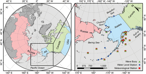
The geomorphological characteristics of coastal Alaska are highly variable, ranging from low-lying deltas on the north and west coasts to complex volcanic topographies in the south (Joyce et al. 2019). In addition, this almost 55,000-km-long shoreline is exposed to contrasting tidal regimes, with microtidal conditions observed in the Beaufort and Chukchi Seas and macrotidal fluctuation in the Pacific and Gulf of Alaska regions. The semi-enclosed Bering Sea is bounded by the Aleutian Islands arc and the Pacific Ocean to its south and the Bering Strait and Chukchi Sea to the north, with a mean tidal range of 0.4 to 1.2 m (Mason, Salmon, and Ludwig 1996). Composed of a deep basin (up to 3,500 m deep) on its southwest half and a shallow continental shelf (<200 m deep) on its northeastern side, the Bering Sea is under the influence of major interannual physical variations due to the Pacific–North American and the Southern Oscillation patterns (Stabeno, Schumacher, and Ohtani 2009). To assess the modeling performance under sea ice–free waters, more emphasis was given to the areas of more significant sea-ice retreat (Figure 1b); that is, Beaufort, Chukchi, and Bering Seas (Koyama et al. 2017).

Figure 1. Study area, including Alaska and Eastern Siberia, as well as the hydrometeorological stations used to assess the hydrodynamic and wave modeling approach.

The region of study is known to be under the influence of major cyclone genesis regions, including the highly active northwest Pacific (Cao, Wu, and Bi 2018), the Eurasian Continent (Day, Holland, and Hodges 2018), and the Arctic Ocean (Lee and Kim 2019). Although under current diminishing patterns, sea ice usually begins forming in November, lasting as late as July, entirely covering the study region from the shelf break of the Bering shelf northwards (Joyce et al. 2019). According to Basu, Zhang, and Wang (2019), Arctic sea ice reaches its minimum extent by late summer and early fall and reaches its maximum by late winter and early spring. Note that due to the current warming conditions, the ice-free water season offshore of northern Alaska has lengthened by up to three months (Walsh et al. 2020). As a result, storms that used to be more frequent and intense during the winter are also becoming a threat in the warmer months (Koyama et al. 2017; Day, Holland, and Hodges 2018; Lee and Kim 2019).

Water level and wave observational data are relatively scarce in western and northern Alaska when compared to other regions of the country. A total of nine National Oceanic and Atmospheric Administration (NOAA) water level stations were selected for model validation. Wave buoy locations for wave model assessment included three National Data Buoy Center wave buoys from the Bering Sea, supplemented by thirteen buoys from the southern Aleutians and Gulf of Alaska (Figure 1). A detailed data description can be found in Supplementary Material Table 1.

Material and methods

Hydrodynamic and wave model setup

The coupled Advanced Circulation and Simulating Waves Nearshore (ADCIRC+SWAN) numerical models were used to simulate the complex nonlinear interactions between astronomical tides, storm surges, and wind wave-induced setup/set-down in the study area described in the previous section. We used the latest version 54, which fixed several bugs present in the previous version, including a correct representation of the surface roughness calculation. The ADCIRC model computes surface water levels and current velocities using the modified shallow-water equations on an unstructured triangular mesh (Luettich, Westerink, and Scheffner 1992). By employing finite element and finite difference numerical methods, the model discretizes its governing equations in space and time (Pandey and Rao 2019). In the present study, total water levels were obtained through a two-dimensional depth-integrated (ADCIRC-2DDI) approach derived from the generalized wave-continuity equations (Dietrich et al. 2011):

(1) $\frac{{\mathrm{\partial }}^2\zeta }{\mathrm{\partial }{t}^2}+{\tau }_0\frac{\mathrm{\partial }\zeta }{\mathrm{\partial }t}+\frac{\mathrm{\partial }{J}_x}{\mathrm{\partial }x}+\frac{\mathrm{\partial }{J}_y}{\mathrm{\partial }y}-UH\frac{\mathrm{\partial }{\tau }_0}{\mathrm{\partial }x}-VH\frac{\mathrm{\partial }{\tau }_0}{\mathrm{\partial }x}=0$(1)

where $U$ and $V$ are the depth-averaged horizontal velocities in their respective $x$ and $\hspace{0.17em}y$ directions; ${\tau }_0$ is a phase propagation optimization parameter; $\zeta$ is the surge, in a given time $t$; and $H$ is the total water depth. $\underset{x}{J}$ and $\underset{y}{J}$ are obtained as

(2) $J_x=-UH\frac{\mathrm{\partial }U}{\mathrm{\partial }x}-VH\frac{\mathrm{\partial }U}{\mathrm{\partial }y}+fVH-\frac{g}{2}\frac{\mathrm{\partial }{\zeta }^2}{\mathrm{\partial }x}-gH\frac{\mathrm{\partial }}{\mathrm{\partial }x}\left[\frac{P_s}{g{\rho }_0}\alpha \eta \right]+\frac{{\tau }_{sx,\hspace{0.17em}wind}+{\tau }_{sx,waves}-{\tau }_{bx}}{{\rho }_0}+\left(M_x-D_x\right)+U\frac{\mathrm{\partial }\zeta }{\mathrm{\partial }t}+{\tau }_{0}UH-gH\frac{\mathrm{\partial }\zeta }{\mathrm{\partial }x}\hspace{0.17em}$(2)

(3) $J_y=-UH\frac{\mathrm{\partial }V}{\mathrm{\partial }x}-VH\frac{\mathrm{\partial }V}{\mathrm{\partial }y}+fUH-\frac{g}{2}\frac{\mathrm{\partial }{\zeta }^2}{\mathrm{\partial }y}-gH\frac{\mathrm{\partial }}{\mathrm{\partial }y}\left[\frac{P_s}{g{\rho }_0}\alpha \eta \right]+\frac{{\tau }_{sy,\hspace{0.17em}wind}+{\tau }_{sy,waves}-{\tau }_{by}}{{\rho }_0}+\left(M_y-D_y\right)+V\frac{\mathrm{\partial }\zeta }{\mathrm{\partial }t}+{\tau }_{0}VH-gH\frac{\mathrm{\partial }\zeta }{\mathrm{\partial }y}\hspace{0.17em}$(3)

where $P$ is the barometric pressure, $f$ is the Coriolis force, $\eta$ is the Newtonian equilibrium tidal potential, $\alpha$ is the effective earth elasticity factor, $g$ is the acceleration of gravity, ${\rho }_0$ is the water density, $D$ is the momentum dispersion term, $M$ is the lateral stress gradient, and ${\tau }_b$, ${\tau }_{s,\hspace{0.17em}waves}$, ${\tau }_{s,\hspace{0.17em}wind}$, are the bottom shear, wave radiation, and free surface stresses, respectively.

The SWAN model is a two-dimensional third-generation wind–wave model that computes wind-generated surface gravity waves according to the action balance equation, considering physical processes such as shoaling, depth-induced breaking, wave–wave interactions, dissipation, and refraction (Booij, Ris, and Holthuijsen 1999; Dietrich et al. 2011). Considering the geographical space ($x$), direction ($\theta$), angular frequency ($\sigma$), and time ($t$), SWAN calculates the wave action density spectrum $N\left(x,t,\sigma ,\theta \right)$ by

(4) $\frac{\mathrm{\partial }N}{\mathrm{\partial }t}+\mathrm{\nabla }\vec{x}\left[\left({\vec{C}}_g+\vec{C}\right)N\right]+\frac{\mathrm{\partial }{C}_{\theta }N}{\mathrm{\partial }\theta }+\hspace{0.17em}\frac{\mathrm{\partial }{C}_{\sigma }N}{\mathrm{\partial }\sigma }=\frac{S_{tot}}{\sigma }\hspace{0.17em}$(4)

where $\vec{C}$ and ${\vec{C}}_g$ are the ambient current and wave velocities, $C_{\theta }$ and $C_{\sigma }$ are the wave energy propagation velocity in the spectral space for the propagation direction $\theta$ and frequency $\sigma$, $\mathrm{\nabla }\vec{x}$ is the gradient operator in the two-dimensional geographic space, and $S_{tot}$ is represents the physical processes that generate, dissipate, or redistribute wave energy.

SWAN wave processes can be divided in four major categories: (i) wave generation, (ii) wave propagation (i.e., refraction, shoaling, diffraction, and reflection), (iii) wave transformation (nonlinear wave–wave interactions), and (iv) wave dissipation (i.e., bottom friction, white capping, and breaking), which are calculated as

(5) $S_{tot}=\hspace{0.17em}{S}_{in}+\hspace{0.17em}{S}_{nl3}+\hspace{0.17em}{S}_{nl4}+\hspace{0.17em}{S}_{wc}+\hspace{0.17em}{S}_{bfr}+\hspace{0.17em}{S}_{surf}\hspace{0.17em}$(5)

where $S_{in}$ is the wind input to wave generation, $S_{nl3}$ and $S_{nl4}$ are the nonlinear three- and four-wave interactions, $\hspace{0.17em}{S}_{wc}$ is the loss of wave energy through white capping, $S_{bfr}$ is the wave energy loss by bottom friction, and $S_{surf}$ is the dissipation via depth-induced wave breaking.

When coupled, the ADCIRC and SWAN models share the same unstructured numerical mesh, thus allowing the model components to be mutually applied in a two-dimensional space (one vertical level). Information is passed between models in five main steps. First, SWAN passes its radiation stresses and their gradients to ADCIRC. Then, ADCIRC solves the generalized wave-continuity equations, extrapolating the wave forcing forward in time. Elements in the numerical mesh are either activated or deactivated by a wetting and drying algorithm as a result of inundation. SWAN is then forced using the updated surface winds, currents, and water levels from ADCIRC by solving its depth-integrated momentum equations. Lastly, the radiation stresses and gradients from SWAN are again passed to ADCIRC as a forcing function. As described by Dietrich et al. (2011), this coupled model stands out for its high computational efficiency and accurate representation of wave–current processes in coastal regions. Considering that the direct effects of waves on storm surge are fundamental for accurate storm surge modeling, as widely discussed in the literature (Dietrich et al. 2011; Bertin et al. 2015; Wu et al. 2018), a stable and highly computationally efficient numerical mesh was developed via the object-oriented OceanMesh2D (Roberts, Pringle, and Westerink 2019; Figure 2).

Figure 2. (a) Developed numerical mesh, with higher resolution in the (b) coast of Alaska. Mesh resolution is given by the distance between nodes in kilometers.

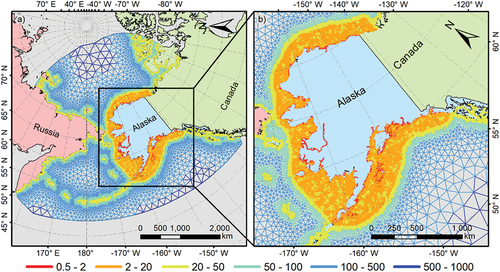
The numerical mesh extends from northern Canada to Eastern Siberia on its northern ocean boundary while going from southern Kamchatka (Russia) to western Canada on its southern Pacific boundary. With a total of 202,525 nodes, the numerical mesh was built in a nested sequence of model domains that allowed the gradual increase of its resolution from more than 500 km in the open ocean to 500 m nearshore. Topo-bathymetric inputs were derived from the General Bathymetric Chart of the Oceans (GEBCO 2019) for the lower resolution areas and nautical charts for higher resolution nearshore domains, all standardized to the MSL vertical datum. Tidal open-ocean boundary conditions followed the constituents defined by Joyce et al. (2019) using the fully global model of ocean tides TPXO 9.1 (Egbert and Erofeeva 2002). Varying bottom friction imposed by the different land covers on the hydrodynamic circulation and shallow water wave energy was attributed to each mesh node. This bottom friction is represented by a given Manning’s n value, which is then translated by ADCIRC as a quadratic friction coefficient in the bottom stress calculation and free surface shear stress (Atkinson et al. 2011). Land cover information was derived from the Global Land Cover Characterization data set based on unsupervised classification of ten-day Normalized Difference Vegetation Index and 1-km Advanced Very High-Resolution Radiometer composites (GLCC 2020). Manning’s n values were attributed following recommendations from Atkinson et al. (2011) and Garzon and Ferreira (2016). Nonlinear bottom friction, finite amplitude terms, convective acceleration, wetting and drying, and the time derivative of convective acceleration are included in the model setup.

Wind and pressure forcing

Wind speed and direction and atmospheric pressure were implemented in ADCIRC+SWAN using a single meteorological forcing input file in a rectangular grid covering the entire model domain. This formulation uses Garret’s formula (Luettich and Westerink 1999) to compute wind stress from the wind speed, interpolating the gridded information in space (onto the numerical mesh) and in time (to synchronize the forcing with the model’s timestep). Seven reanalysis products, provided by multiple meteorological agencies worldwide were assessed based on their temporal availability (i.e., encompassing the selected storms) and spatial attributes (i.e., covering the model domain). A detailed description of all forcings used is presented in Table 1.

Table 1. Available wind and pressure forcing products implemented in the proposed ADCIRC+SWAN model

Reanalysis product	Temporal coverage		Spatial resolution^a		Reference
	Initial	Final	Latitude	Longitude
ECMWF-ERA5	1979	Current	0.25°	0.25°	Hersbach et al. (2020)
NCEP-CFSv2	2011	Current	0.2045°	0.2045°	Saha et al. (2014)
NOAA-NOGAPS	1997	2008	1°	1°	Hogan and Rosmond (1991)
JMA-JRA55	1958	Current	1.25°	1.25°	Kobayashi et al. (2015)
NASA-MERRA2	1980	Current	0.5°	0.625°	Gelaro et al. (2017)
NCEP-GFS	2004	Current	0.5°	0.5°	Yang et al. (2006)
NOAA-CIRESv3	1981	2015	1°	1°	Slivinski et al. (2019)

Note. ^a At 60° N, a resolution of 1° × 1° is equivalent to an approximately 60 km × 60 km grid at ground level.

The ECMWF-ERA5 global climate reanalysis was significantly improved, relative to its predecessor ERA-Interim (0.75° × 0.75°). ERA5 is derived from the Integrated Forecasting System version Cy41r2, which is used as a starting point for the production of reanalysis data sets (Dullaart et al. 2020). An ensemble hybrid four-dimensional variation assimilation system that includes more variables than its predecessors is used for data assimilation (Tahir et al. 2020). Lastly, all ERA5 ocean-wave-atmosphere and land–atmosphere interactions are coupled (Hersbach et al. 2020). The resulting product has a spatial resolution of 0.25° by 0.25°, accounting for 137 vertical layers at hourly intervals (Hersbach et al. 2020).

The Climate Forecast System version 2 (CFSv2) has run operationally since its release in March 2011 (Gramcianinov et al. 2020). The CFSv2 predecessor, CFSR (at 6-hourly outputs on a 0.5° × 0.5° grid), is applied over a thirty-two-year period (1979–2010) as initial conditions for a reforecast starting in 1982, which is used to improve seasonal and subseasonal CFSv2 estimates (Saha et al. 2014). The fully coupled ocean–land–atmosphere final products are built upon the Climate Data Assimilation System, resulting in sixty-four sigma-pressure vertical layers at a spatial resolution of 0.2045° (Saha et al. 2014).

The Navy Operational Global Atmospheric Prediction System (NOGAPS) model is an older product provided in a coarser resolution (1.0° by 1.0°) covering a short period from 1997 to 2008. Vertical resolution ranges from eighteen to twenty-eight pressure levels for atmospheric model variables and thirty-four depth levels for the ocean model variables in addition to its at surface layer (Hogan and Rosmond 1991). In an even coarser spatial resolution (1.25° × 1.25°), the Japan Meteorological Agency (JMA) provides what is the longest third-generation reanalysis data set available (from 1958 to the present). The Japanese Reanalysis 55-year (JRA55) also uses a 4D-Variational Data Assimilation scheme with variational bias correction in a 3-hourly output timestep (Tahir et al. 2020). Released in 2013, the JRA55 has a total of sixty levels and was described in detail by Kobayashi et al. (2015).

The second version of the National Aeronautics and Space Administration (NASA) atmospheric reanalysis MERRA2 (Modern-Era Retrospective analysis for Research and Applications version 2) was the first product to represent aerosols interactions with physical climate process using space-based observations (Kim, Kim, and Kang 2018). MERRA2 was built from the combination of the Goddard Earth Observing System Model V5 and Atmospheric Data Assimilation System. Its spatial resolution is 0.625° and 0.5° for longitudinal and latitudinal spacing, respectively. It uses a 3D-Var data assimilation scheme (Gelaro et al. 2017) and provides hourly output from 1980 to the present.

The coupled model Global Forecast System (GFS) is composed of ocean, land–soil, sea ice, and atmospheric models that cover the globe in varying resolutions (13 km, 0.25°, 0.5°, and 1°) but are available as analysis only at 0.5° (from January 2007) or 1° (from March 2004; Garzon, Ferreira, and Padilla-Hernandez 2018). This global spectral numerical model derived from the primitive dynamical equations that include parameterizations for atmospheric physics is output every 6 hours and comprises sixty-four sigma layers (Yang et al. 2006; Garzon, Ferreira, and Padilla-Hernandez 2018). A detailed description of GFS attributes is found in Yang et al. (2006).

Lastly, the Twentieth Century Reanalysis (20CR) project by NOAA, the Cooperative Institute for Research in Environmental Sciences (CIRES), and the U.S. Department of Energy (DOE) was the first to ensemble subdaily global atmospheric conditions spanning over 100 years (Slivinski et al. 2019). Data assimilation is based on an ensemble Kalman filter method, with background first-guess fields supplied by weather model forecasts (Wang et al. 2013). Upgrades on the data assimilation method based on a larger set of observations as well as the use of a higher-resolution forecast model have improved the representations of storm intensity, diminished the sea-level pressure bias, and removed spin-up effects observed in its predecessor (Slivinski et al. 2019). The new NOAA-CIRES-DOE 20CR V3 (hereafter called CIRESv3) is available from 1981 to 2015 at 3-hourly intervals with a spatial resolution of 1° for twenty-eight pressure levels.

In order to establish a fair temporal comparison between these products, wind and pressure fields were input to the ADCIRC+SWAN model in a timestep equal to that of the products with the lowest temporal resolution (i.e., 6 hours).

Selected Storms

The storm surge and wave assessment using the wind and pressure forcings presented in Table 1 was carried out during three storms in the Bering Sea, selected based on their magnitudes and data availability (Supplementary Material Table 1) for periods of open water within the model domain. Therefore, because these storms hit the study area during the ice-free conditions, sea ice was not considered in the ADCIRC+SWAN model. According to Wicks and Atkinson (2017), the most common surge pattern in the region occurs as a response to deep systems moving from the Pacific toward the eastern or central parts of the northern Bering Sea. Following this pattern, the first selected storm (hereafter called Storm 1) hit the western coast of Alaska by early October 2019, leading to peak surges of more than 1.7 m in Unalakleet, Alaska (63.87° N, −160.78° E). In a thirty-year descriptive analysis of extreme storm surges in the Bering Sea, Erikson et al. (2015) ranked the thirty largest maximum water levels, with the largest reaching more than 3 m and the lowest less than 1.5 m. Storm 1 was therefore selected as a representative case of a mid-intensity event. The storm progression in terms of wind speed and direction and MSL pressure is depicted in Figure 3a.

Figure 3. Storm progression in terms of wind magnitude and speed and MSL pressure during (a) Storm 1, (b) Storm 2, and (c) Storm 3.

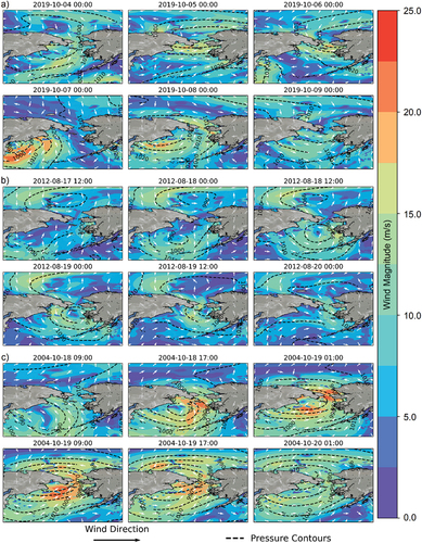
Storm 2 (Figure 3b) was chosen as a lower intensity event that made landfall in western Alaska by mid-August 2012. Moving in the Bering Sea from west to east, the storm consisted of predominately southern winds, leading to significant water levels in large parts of the coastline (Joyce et al. 2019), passing the 0.75 m mark in the Norton Sound gauge (64.50°N, 165.44°W). This storm was also analyzed by Joyce et al. (2019) and was used as a basis for model performance comparison.

The third storm caused one of the largest positive surges ever recorded in western Alaska (Erikson et al. 2015; Wicks and Atkinson 2017). The storm began to form three days prior to the development of maximum water levels as a low-pressure system in Eastern Siberia. MSL atmospheric pressures dropped significantly on October 18 as the system progressed northeastwards, eventually reaching 950 hPa on October 19 (Wicks and Atkinson 2017). The storm stalled and slowly dissipated in the Bering Strait region for the next two days (Figure 3c). The 2004 Bering Strait Storm (Storm 3) significantly impacted the town of Kivalina, Alaska, causing flooding and shoreline retreat of 12 m, as well as damaging the town’s sewage system (Fang et al. 2018). The damage led the Federal Emergency Management Agency to declare Kivalina to a major disaster area.

Model assessment

All of the reanalysis data used for model forcing were assessed by comparing calculated and observed surge and wave data (Supplementary Material Table 1). The two-dimensional Taylor diagram (Taylor 2001) was used to summarize model performance in terms of the magnitude and phase of model error. The degree of correspondence between observed and modeled storm surge and waves was then depicted as a function of root mean square error (RMSE), correlation coefficient ($r$), and standard deviation, defined as follows:

(6) $RMSE=\hspace{0.17em}{\left[\frac{{\sum }_{i=1}^n{\left(P_i-O_i\right)}^2}{n}\right]}^{\frac{1}{2}}\hspace{0.17em}$(6)

(7) $r=\hspace{0.17em}\frac{{\sum }_{i=1}^n\left(O_i-\bar{O}\right)\left(P_i-\bar{P}\right)}{\sqrt{{\sum }_{i=1}^n{\left(O_i-\bar{O}\right)}^2{\sum }_{i=1}^n{\left(P_i-\bar{P}\right)}^2}}\hspace{0.17em}$(7)

where $\hspace{0.17em}{P}_i$ and $O_i$ are the predicted and observed values for the $i$ timestep of a total size $n$ and $\bar{P}$ and $\bar{O}$ are their respective averages. When interpreting the Taylor diagram, the RMSE is given by the distance from the reference observed point on the x-axis, $r$ is represented by the azimuthal point position, and the standard deviation is proportional to the radial distance from the origin (Taylor 2001). Following recommendations from Garzon, Ferreira, and Padilla-Hernandez (2018), individual station results were average into their respective forcing scenarios after being normalized by the observed standard deviation.

Results

Storm surge

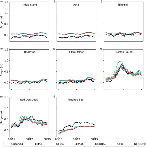
As described in Supplementary Material Table 1, water level observations are available for nine locations in western and northern Alaska during Storm 1. In addition, five reanalysis products were used to provide forcing for the October 2019 storm (Table 1). As depicted in Figure 3a, Storm 1 mostly impacted the northern Bering Sea. Therefore, little to no surge was expected in the vicinity of the Aleutian Islands (Figures 4a–4e) and northern Alaska (Figure 4i). Model simulations correctly predicted significant surges only at Unalakleet, Norton Sound (in the Port of Nome), and Red Dog Dock stations (Figures 4f–4h).

Figure 4. Observed and simulated storm surges (total water level − tides) for all available wind and pressure forcings during Storm 1.

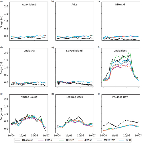
The most significant surges were observed at Unalakleet on the eastern side of the Norton Sound. When forced with CFSv2, modeled surges were slightly overestimated for maximum conditions, eventually surpassing the 2 m mark for the highest surge peak (Figure 4f). All other reanalysis products led to model underestimations at Unalakleet, with the smallest errors observed for GFS, followed by MERRA2, ECMWF (ERA5), and JMA (JRA55), respectively. CFSv2-driven model results for the western portion of the Norton Sound (Figure 4g) also seem more accurate than those forced with other products. JRA55 and GFS slightly underestimated the maximum surge conditions, followed by MERRA2 and ERA5. Thirdly, all five products generated almost 0.5 m underpredictions of surge at the Chukchi Sea station at Red Dog Dock (Figure 4h), with estimates closest to observations obtained from JRA55 and CFSv2. Finally, we note that, regardless of the analysis product used for forcing, the model was not able to capture the more than half-meter surge observed at Prudhoe Bay in the Beaufort Sea (Figure 4i).

With higher minimum atmospheric pressures and lower wind speeds, Storm 2 had an overall lower intensity than Storm 1 (Figure 3b). Nevertheless, because Storm 2 made landfall in the vicinities of the Bering Strait, observed surges at the Norton Sound and Red Dog Dock stations were almost as high as those of Storm 1 (Figures 5f, 5g). As with Storm 1, CFSv2-based hydrodynamic simulations tended to overestimate maximum surge height (Figures 5f, 5g). In addition, simulations with GFS and CFSv2 forcing generated more accurate surge estimates compared to those from JRA55, MERRA2, ERA5, and CIRESv3. Equally better model performances at Prudhoe Bay (Figure 5h) were found for all forcings. However, consistent underestimation was still present, which may be an indication of another source of uncertainty such as changes in the bathymetry or systematic errors in observations.

Figure 5. Observed and simulated storm surges (total water level − tides) for all available wind and pressure forcings during Storm 2.

Storm 3, which occurred in October 2004, is the most extreme storm considered in the present study. Therefore, the storm’s character is significant for several applications, including flood hazards mitigation, maritime navigation, and offshore and coastal engineering. However, the number of observational data sets, as well as state-of-the-art atmospheric forcings available, is considerably limited for 2004. In addition, bathymetry-derived errors may hamper model performance because it is highly sensitive to nearshore morphological changes over time (Dullaart et al. 2020). Results for Storm 3 were compared against the five available water level stations data for October 2004 (Figure 6).

Figure 6. Observed and simulated storm surges (total water level − tides) for all available wind and pressure forcings during Storm 3.

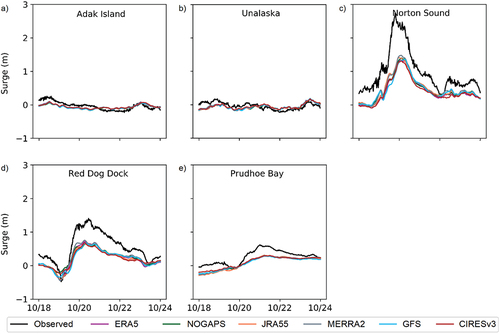
The simulations of Storm 3 resulted in reasonably accurate results at the stations in the Aleutian arc (Figures 6a, 6b). Recall that with Storms 1 and 2, the surge model tended to overpredict surge height at these stations (Figures 4 and 5). In the Norton Sound station, on the other hand, surge estimates for all forcings were largely underpredicted, missing the maximum peak by almost 1.5 m (Figures 6d). Likewise, all of the different atmospheric forcing–derived results significantly underestimated the surge conditions at the Red Dog Dock station (Figure 6d). As described in Table 1, the best performing product for Storms 1 and 2, CFSv2, is not available for periods prior to 2011. The remaining model simulations, including those from the discontinued NOGAPS product, showed very similar results at all stations considered. A statistical assessment of surge simulations under different model forcing setups is presented in the Skill metrics assessment section.

Waves

During Storm 1, large significant wave heights (H_s) followed the surge peaks (Figure 4), especially within the Bering Sea extent, including stations at Nome (Figure 7c), central Bering Sea (Figure 7e), and southwest Bering Sea (Figure 7p). For these three stations, CFSv2 results resemble the observations not only on its representation of peak but also the overall H_s fluctuation patterns. Forcing based on the other reanalysis products led to significant H_s underestimation, with the largest underestimates given by MERRA2, JRA55, and ERA5 and the smallest by GFS (Figures 7c, 7e, 7p).

Figure 7. Observed and simulated H_s for all available wind and pressure forcings during Storm 1.

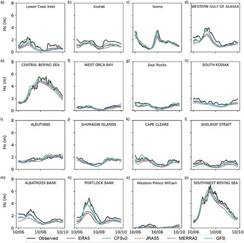
Sites outside the Bering Sea also experienced large H_s for the four-day period considered. Buoys at Western Gulf of Alaska (Figure 7d) and Portlock Bank (Figure 7n) in the Gulf of Alaska (see Supplementary Material Table 1) registered maximum H_s higher than 4 m, with GFS and CFSv2 generating relatively accurate results. All of the other forcings led to underestimations up to 2 m lower than those from CFSv2 and GFS. In all other buoys where wave regimes remained steady, all modeling results are relatively similar and no significant difference can be visually identified.

For Storm 2 (August 2011), only half of the total number of buoys used for Storm 1 are available. Even though a larger number of buoys were monitoring wave condition in 2011 (Supplementary Material Table 1), many of them had data gaps, which limited their usefulness in the present analysis. For instance, only two buoys are available for the whole Bering Sea extent, with one of them (central Bering Sea, Figure 8b) having what appears to be a bias error, which therefore was not used in the following assessments.

Figure 8. Observed and simulated H_s for all available wind and pressure forcings during Storm 2.

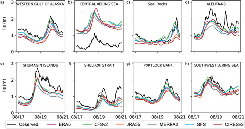
As expected, this smaller intensity storm resulted in smaller H_s when compared to Storm 1. Significant wave heights higher than 2.5 m were only observed in two buoys in the Pacific side of the Aleutian Arc (Figures 8d, 8e), whereas H_s slightly higher than 2 m was observed within the Bering Sea domain (Figure 8h). Although under higher wind speed regimes due to its proximity to the moving cyclone and the increased fetch during ice-free conditions, wind waves at the semi-enclosed Bering Sea (Figure 8h) may not be as high as those in the open Pacific Ocean side (e.g., Figures 8d, 8e) given the limitations in fetch imposed by the Aleutian Islands as well as eastern Russia and Alaska. Once again, CFSv2-driven simulations provided the most accurate wave height calculations at the majority of the wave buoy sites (Figures 8a, 8c, 8g, 8h). However, it is noteworthy that closer peaks were modeled for CIRESv3, JRA55, and MERRA2 at buoys in the Aleutians coast (Figure 8d), Shumagin Islands (Figure 8e), and Shelikof Strait (Figure 8f), respectively. Finally, it should be noted that all of the reanalysis products led to H_s underestimations at all monitored locations (Figure 8).

Comparable H_s patterns were also observed during the higher intensity Storm 3 (Figure 9). Having maximum H_s of over 8 m, higher waves were observed at a buoy in the Pacific Ocean side (e.g., Western Gulf of Alaska; Figure 9a) than on the Bering Sea (Figure 9b). Outside the Bering Sea domain, all six forcings (ERA5, NOGAPS, JRA55, MERRA2, GFS, CIRESv3) resulted in waves smaller than observations. In the central Bering Sea buoy, however, slight overestimations were modeled when forced with JRA55 and CIRESv3 (Figure 9b).

Figure 9. Observed and simulated H_s for all available wind and pressure forcings during Storm 3.

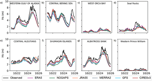
The coarser resolution products MERRA2, CIRESv3, and JRA55 led to the highest H_s estimated peaks in the stations where the most significant wave heights were observed (Figures 9a, 9b, 9e, 9f, and 9g). Moreover, the discontinued NOGAPS seemed to underperform the other forcings for at least two sites (Figures 9a and 9f). Given the heterogeneity in the quality of modeled results as a function of the selected forcing, a simple visual qualitative analysis was not capable of identifying the most adequate atmospheric forcing throughout different storms and spatially distributed locations. Therefore, the following section develops a quantitative model assessment for the maximum surge and H_s peaks as well as for its oscillations.

Skill metrics assessment

Figure 10 depicts the Taylor diagram of all water level stations (Figures 10a–10c) and wave buoys (Figures 10d–10e) during the three storms, as well as their mean positioning as a result of the skill metric averages among stations. For the surge results in Storm 1 (Figure 10a), all forcings led to similarly phased estimates, because all modeling scenarios had average $r$ values around 0.4. Given their position in relation to the reference dashed line, one can assume that CFSv2 and GFS have the estimates closest to observation in terms of amplitude, with GFS giving a slightly higher and CFSv2 gives a slightly smaller surge amplitude. Even smaller amplitudes were obtained for MERRA2, JRA55, and ERA5. The higher amplitude of GFS corroborates what is observed in Figures 4a–4e for stations under low surge conditions.

Figure 10. Taylor diagram of (a)–(c) surges and (d)–(f) waves for individual stations (small “x”) as well as averaged by storm (large “x”). The blue triangle indicates the observed data.

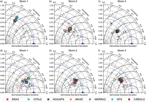
For Storm 2 (Figure 10b) and Storm 3 (Figure 10c), all modeling scenarios have standard deviations smaller than that of observations and $r$ values within the 0.7 to 0.8 range. Larger amplitudes were observed for JRA55 during Storms 2 and 3, which corroborates Figures 5f, 5g, and6c, 6d, where JRA55 often starts as one of the lowest surges but as the storm progresses it provides one of the highest water levels. This more pronounced magnitude sensitivity of JRA55 is particularly interesting given the fact it has the coarser spatial resolution (1.25°) considered in the present study (Table 1). During Storm 3, all forcings have barely distinguishable results. In order to quantitatively estimate the error associated with each one of the products, RMSE was calculated at all stations and for all scenarios (Table 2).

Table 2. Storm surge RMSE (in meters) for each station and storm for all forcings considered

		Atmospheric forcing
	Station	ERA5	CFSv2	NOGAPS	JRA55	MERRA2	GFS	CIRESv3
Storm 1	Adak Island	0.10	0.11	—	0.10	0.10	0.11	—
	Atka	0.10	0.11	—	0.11	0.11	0.12	—
	Nikolski	0.17	0.18	—	0.17	0.18	0.18	—
	Unalaska	0.12	0.12	—	0.12	0.12	0.13	—
	St. Paul Island	0.11	0.12	—	0.11	0.12	0.12	—
	Unalakleet	0.42	0.21	—	0.46	0.32	0.22	—
	Norton Sound	0.17	0.14	—	0.14	0.15	0.11	—
	Red Dog Dock	0.16	0.12	—	0.13	0.14	0.14	—
	Prudhoe Bay	0.30	0.29	—	0.30	0.29	0.30	—
	Average Storm 1	0.18	0.16	—	0.18	0.17	0.16	—
Storm 2	Adak Island	0.13	0.13	—	0.12	0.13	0.13	0.12
	Atka	0.15	0.15	—	0.15	0.15	0.15	0.14
	Nikolski	0.06	0.06	—	0.06	0.06	0.06	0.05
	Unalaska	0.08	0.08	—	0.08	0.08	0.08	0.07
	St. Paul Island	0.08	0.10	—	0.08	0.08	0.09	0.07
	Norton Sound	0.15	0.22	—	0.14	0.15	0.17	0.13
	Red Dog Dock	0.11	0.14	—	0.11	0.11	0.10	0.13
	Prudhoe Bay	0.17	0.15	—	0.17	0.16	0.16	0.16
	Average Storm 2	0.12	0.13	—	0.11	0.12	0.12	0.11
Storm 3	Adak Island	0.09	—	0.10	0.10	0.09	0.10	0.09
	Unalaska	0.10	—	0.10	0.11	0.10	0.11	0.10
	Norton Sound	0.65	—	0.60	0.59	0.57	0.63	0.66
	Red Dog Dock	0.38	—	0.39	0.40	0.36	0.41	0.42
	Prudhoe Bay	0.19	—	0.20	0.20	0.19	0.20	0.18
	Average Storm 3	0.28	—	0.28	0.28	0.26	0.29	0.29
	Total average	0.18	0.14	0.28	0.18	0.17	0.17	0.18
	% RMSE	28.57	—	100	28.57	21.14	21.14	28.57

Note. Lowest RMSEs are presented in bold and stations within the Bering and Chukchi Seas are in italics.

As presented in Table 2, as well as Figures 4a–4e, ERA5 resulted in slightly better surge estimates at regions that were not directly impacted by cyclone-driven surges. Nevertheless, at extreme conditions, ERA5 led to larger uncertainties, reaching errors twice as large at Unalakleet (Table 2) compared to that for the best-fit model simulations; that is, CFSv2. The lowest average RMSEs during Storm 1 were obtained from GFS and CFSv2 (both at 0.16 m); MERRA2, JRA55, and ERA5 had average RMSEs of 9.29 percent, 17.15 percent, and 17.86 percent higher than CFSv2, respectively. In contrast, for the lower intensity Storm 2, smaller RMSE was obtained from CIRESv3, followed by JRA55, MERRA2, ERA5, GFS, and CFSv2. Surge RMSEs obtained in the present study are comparable to those from Joyce et al. (2019), who found slightly inferior model performance at the Norton Sound station (RMSE = 0.15 m) and slightly superior results at Prudhoe Bay (RMSE = 0.09 m; Table 2). Lastly, errors during Storm 3 were more constant within products, with RMSE roughly falling under the 10 percent mark in comparison to the lowest error forcing; that is, MERRA2 at 0.26 m. In Table 2 it is also shown the overall RMSE averaged from all stations during the three storms. When using ERA5, JRA55, MERRA2, or GFS, ADCRIC+SWAN simulations showed surge RMSE 20 percent larger than that from CFSv2, reaching average errors up to 0.28 m. This significant percentage error reinforces the need to assess the implication of choosing different wind and pressure fields due to the high model sensitivity to what is considered one of its most influential inputs (Lakshmi et al. 2017; Chu et al. 2019; Torres et al. 2019).

When assessing H_s via Taylor diagram, one can infer that, similar to storm surge, wave model performance is improved in terms of amplitude when forced with CFSv2 (Figure 10). Although smaller than the observed standard deviation, CFSv2-driven average results fall closer to the reference dashed line (Figures 10d, 10e), yet wave results tend to be more in phase with observations when forced with ERA5 and GFS, because they have higher $r$ values (Figures 10d, 10e). ERA5’s superior phase representation, expressed in terms of higher $r$ values, is also seen during Storm 3. Generally, H_s errors (Figures 10d–10f) are smaller than those observed for surge (Figures 10a–10c), showing that other sources of uncertainties not evaluated in the present study may play a more accentuated role over surge than over wave simulations. It is also worth mentioning that wave simulations in the study area seem to be more sensitive to spatial resolution than those of surge, because the higher resolution products (ERA5, CFSv2, and GFS) often give the best wave estimates.

According to Table 3, average H_s RMSE for all three events varied from 0.33 to 0.86 m as a function of wind and pressure forcing. The higher spatial resolution CFSv2 led to the lowest error estimates, followed by GFS (32.74 percent higher RMSE), ERA5 (35.25 percent higher RMSE), JRA55 (48.39 percent higher RMSE), CIRESv3 (60.92 percent higher RMSE), and NOGAPS (157.55 percent higher RMSE; Table 3).

Table 3. H_s RMSE (in meters) for each buoy and storm for all forcings considered

		Atmospheric forcing
	Wave buoy	ERA5	CFSv2	NOGAPS	JRA55	MERRA2	GFS	CIRESv3
Storm 1	Lower Cook Inlet	0.50	0.49	—	0.65	0.67	0.47	—
	Kodiak	0.50	0.55	—	0.53	0.73	0.41	—
	Nome	0.35	0.24	—	0.38	0.32	0.22	—
	Western Gulf of Alaska	0.58	0.46	—	0.63	0.76	0.47	—
	Central Bering Sea	0.46	0.49	—	0.41	0.62	0.42	—
	West Orca Bay	0.15	0.16	—	0.23	0.15	0.17	—
	Seal Rocks	0.22	0.24	—	0.33	0.29	0.26	—
	South Kodiak	0.39	0.33	—	0.33	0.49	0.33	—
	Aleutians	0.21	0.30	—	0.29	0.28	0.21	—
	Shumagin Island	0.23	0.22	—	0.19	0.29	0.19	—
	Cape Cleare	0.31	0.32	—	0.48	0.43	0.28	—
	Shelikof Strait	0.26	0.33	—	0.35	0.52	0.42	—
	Albatross Bay	0.46	0.44	—	0.48	0.73	0.44	—
	Portlock Bank	0.86	0.51	—	1.08	1.11	0.55	—
	Western Prince William	0.18	0.21	—	0.14	0.22	0.23	—
	Southwest Bering Sea	0.52	0.49	—	0.45	0.73	0.47	—
	Average Storm 1	0.39	0.36	—	0.43	0.52	0.35	—
Storm 2	Western Gulf of Alaska	0.25	0.20	—	0.36	0.33	0.24	0.43
	Central Bering Sea	—	—	—	—	—	—	—
	Seal Rocks	0.17	0.21	—	0.29	0.25	0.15	0.39
	Aleutians	0.37	0.35	—	0.44	0.57	0.41	0.45
	Shumagin Island	0.44	0.41	—	0.43	0.61	0.43	0.45
	Shelikof Strait	0.29	0.34	—	0.35	0.41	0.45	0.45
	Portlock Bank	0.24	0.16	—	0.32	0.25	0.20	0.32
	Southwest Bering Sea	0.23	0.23	—	0.24	0.30	0.20	0.18
	Average Storm 2	0.28	0.27	—	0.35	0.39	0.30	0.38
Storm 3	Western Gulf of Alaska	1.08	—	1.50	1.22	1.26	1.28	1.21
	Central Bering Sea	1.21	—	1.09	0.87	1.17	0.95	0.89
	West Orca Bay	0.14	—	0.32	0.25	0.21	0.26	0.24
	Seal Rocks	0.47	—	0.62	0.72	0.63	0.61	0.59
	Aleutians	0.79	—	0.69	0.72	0.82	0.68	0.61
	Shumagin Island	0.86	—	1.27	0.94	1.00	1.07	0.72
	Albatross Bay	1.05	—	1.12	1.06	1.24	1.06	0.94
	Western Prince William	0.23	—	0.27	0.20	0.25	0.21	0.19
	Average Storm 3	0.73	—	0.86	0.75	0.82	0.77	0.67
	Total Average	0.45	0.32	0.86	0.50	0.57	0.44	0.54
	% RMSE	35.25	—	157.55	48.39	70.41	32.74	60.92

Note. The lowest RMSEs are presented in bold and buoys within the Bering and Chukchi Seas are in italics.

For Storm 1, the average RMSE for GFS, CFSv2, and ERA5 was at 0.35, 0.36, and 0.39 m, respectively. More pronounced errors were observed for JRA55 and MERRA2, reaching more than 0.43 and 0.52 m. In contrast, during Storm 2, the lowest RMSE was found for CFSv2, followed by 4.73 percent and 9.47 percent larger errors computed for ERA5 and GFS. Similar to Storm 1, wave simulation errors when forced with coarser resolution products, including JRA55, CIRESv3, and MERRA2, were substantially higher; that is, by 27.89 percent, 40.53 percent, and 43.16 percent, respectively. Finally, the largest errors were obtained for Storm 3. Surpassing the 8 m mark (Figure 9a), average RMSE during Storm 3 was as high as 0.86 m for the NOGAPS, decreasing to 0.67 m when using CIRESv3. Overall, the lowest average RMSEs were provided by the highest resolution products, CFSv2, GFS, and ERA5, respectively (Table 3).

As stated by Walsh et al. (2020), the greatest impacts of climate change on natural hazards—for instance, the increasing cyclone-driven surge and waves (Mori et al. 2019)—originate from extreme conditions rather than mean trends. Therefore, properly capturing the peak surge and H_s is pivotal to the success of any coastal hazards–related mitigation practice. Figure 11 depicts the scatterplots of the differences between observed and simulated peak surge (Figures 11a–11c) and H_s (Figures 11d–11f) under all atmospheric forcings and for all three storms.

Figure 11. Peak (a)–(c) surge and (d)–(f) H_s for each monitored station during (a), (d) Storm 1, (b), (e) Storm 2, and (c), (f) Storm 3.

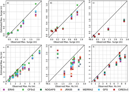
For Storms 1 and 2, the largest differences between surge simulations are seen for stations where the most extreme conditions were observed (Figures 11a, 11b). For instance, during Storm 1 (Figures 11a) and for storm surge higher than 0.7 m, CFSv2-driven peak simulations were higher than those from other forcings. Similarly, for Storm 2, little to no difference was observed for surges lower than 0.6 m, whereas closer to the reference line estimates were computed for CFSv2 during larger surges. On the other hand, little variations between forcings were observed for Storm 3, thus corroborating the Taylor diagram results in Figure 10c. A clear improvement in H_s peak modeling during Storms 1 and 2 was also identified when using CFSv2, where it provides closer to the reference line peak estimates for buoys where the largest waves were observed (Figures 11d, 11e). For Storm 3, CIRESv3, which obtained the lowest overall RMSE (Table 3), also provided the best peak H_s estimates (Figure 11f).

Discussion

Western Alaska and Eastern Siberia are among the most surge wave–dependent coasts in the world (Marcos et al. 2019). Results suggest an overall better model performance for both storm surge and waves when using the higher resolution CFSv2, followed by GFS. Improved surge representations as a function of finer horizontal resolutions were also observed in various other regions (Garzon, Ferreira, and Padilla-Hernandez 2018; Bloemendaal et al. 2019). Similarly, it is also anticipated that more adequate wave simulation will be obtained from higher spatial resolution forcings (Bento, Salvação, and Carlos Soares 2018; Casas-Prat, Wang, and Swart 2018; Gramcianinov et al. 2020). According to Murty et al. (2020), global atmospheric forcings, such as those used in this study, often underestimate wind magnitude near the inner core of the cyclonic system. This source of inaccuracy is intrinsically dependent on the structure of reanalysis products themselves, which at coarser resolutions are incapable of capturing features of depression, size, intensity, and track of cyclones (Lakshmi et al. 2017; Bloemendaal et al. 2019).

However, resolution is not the only factor influencing the applicability of a certain input toward ocean modeling. As stated by Viitak et al. (2020), atmospheric forcing resolution does not have as significant impact on wave modeling as the accuracy of the input wind direction and magnitude. Although significantly better than its predecessors, which were known for underestimating wind magnitudes (Murty et al. 2020), the higher resolution ECMWF-ERA5 was not able to provide accurate storm surge and wave estimates under more intense atmospheric conditions (Figures 10, 11). In order to assess the ERA5 source of uncertainties, a Taylor diagram and peak, MSL pressure, and wind scatterplots are presented Supplementary Material Figures 1 and 2 for the meteorological stations shown in Figure 1. As depicted in Supplementary Material Figure 1, ERA5 shows better representations of wind and pressure, because it is both in phase and havs similar amplitude as the observations. However, for extreme peak conditions—that is, observed wind speed greater than 12 m/s during Storm 1 (Supplementary Material Figure 2d) and Storm 2 (Supplementary Material Figure 2e)—ERA5 underperforms even coarser-resolution products. This misrepresentation of higher intensity winds may be the leading cause for the poorer surge and wave estimates obtained when using ERA5, as presented in the previous sections (Figure 9; Tables 2, 3). Our findings corroborate those of Gramcianinov et al. (2020) in a study applied to the entire Atlantic Ocean that concluded that CFSv2 provides more intense cyclones than ERA5, especially in terms of higher extreme intensity winds. Similarly, ERA5-based surge and wave underestimations were observed by de Lima et al. (2020) in the southern coast of Brazil, even when compared to coarser resolution forcings; for example, GFS. However, it is worth mentioning that ERA5 has proven to be highly accurate for hydrodynamic and wave modeling forcing in studies applied to different parts of the world (Dullaart et al. 2020; Hersbach et al. 2020; Oliveira, Cagnin, and Silva 2020), especially when its high winds are bias corrected (Alday et al. 2021). Thus, the results presented in this study are site specific and should not be extrapolated to other regions. The contrasting results obtained by similar global reanalysis assessments worldwide highlight the importance of the framework proposed in the present study, especially when considering that such an approach has not been previously applied to the western and northern Alaskan coasts.

According to Bloemendaal et al. (2019), contrasts between surge estimates from atmospheric forcings of different resolution increase as a function of magnitude. This behavior is clearly seen in Figures 11a, 11b. During Storm 3 (Figure 11c), coarser resolution forcings are more predominantly available. Even though Storm 3’s magnitude is substantially higher, surge differences between products are not as evident as for Storms 1 and 2. In addition to spatial resolution, the overall poorer model performance during Storm 3 may be attributed to the lack of observational data (Supplementary Material Table 1), which is significantly reduced for past events and thus can influence the data assimilation approach used by the various reanalysis. Furthermore, the use of some forcings, especially from products that are long discontinued or not recently updated, may hamper the surge and wave modeling because modern reanalysis products provide better intercomparisons than older ones (Gramcianinov et al. 2020). It should also be stressed that the considered forcings come in different temporal resolutions. It is known that the proposed modeling framework is more sensitive to spatial than temporal atmospheric forcing resolution (Schaeffer et al. 2011). So, to isolate the effects of the former and to establish a more adequate mean of comparison, all products were temporally resampled to 6 hours timesteps. Therefore, it is expected that estimates superior to those presented in this study may be obtained for the higher temporal resolution products when used to their full temporal capacity.

Identifying the most suitable forcing for events such as those presented in the Results section is crucial for future hydrodynamic and wave modeling studies in the Arctic. According to Cao, Wu, and Bi (2018), the northwest Pacific is known to be the most cyclogenesis-active basin on the planet. It is natural that a fraction of such storms such as the storms evaluated in this study (Figure 3) have poleward tracks through the Bering Sea. However, due to the warming of Arctic waters and the diminishing of sea-ice extent, the frequency and magnitude of storms are projected to rise, especially for the warmer seasons (i.e., summer and early fall) in western and northern Alaska (Mioduszewski, Vavrus, and Wang 2018). When combined with the corresponding longer length of the open-water season, which has increased from one to three months in northern Alaska (Walsh et al. 2020), one may anticipate that assessing events such as those adopted in this study is essential for a vast range of coastal hazards and maritime and environmental engineering and management future practices.

Conclusion

This study presents an assessment of the two-way coupled ADCIRC+SWAN surge and wave outputs when forced with different wind and pressure reanalysis products. Due to the new norm of longer and more synoptically intense warm season in the Arctic, performing extreme surge and wave simulations during sea ice–free conditions is of increasing interest. With a model domain consisting of part of the northern Pacific Ocean, as well as the Bering and Chukchi Seas, the hydrodynamic and wave modeling framework proposed in this study was successfully implemented. The model results are, in some instances, superior to those from previous analyses, while still using a highly computationally efficient 202,525-node numerical mesh.

Model performance for the different forcings was assessed in terms of overall best fit using the Taylor diagram, skill metric statistics, and maximum peak comparison. The highest spatial resolution product CFSv2 available for Storms 1 and 2 and GFS available for Storms 1, 2, and 3 led to the overall most accurate model simulations, performing particularly well at locations exposed to extreme surge and waves. The higher resolution ECMWF-ERA5 provided the most adequate model estimations under low-intensity conditions. However, this product resulted in significantly underestimated surges and waves near the track of the cyclones. Therefore, although at high resolution ERA5 may not be the most appropriate forcing for storm surge and wave hindcasting in the western and northern Alaskan coast, further assessment showed that despite being accurate in the representations of wind and pressure magnitudes, this product underestimates maximum peak wind speeds, which may have caused the ADCIRC+SWAN model to misrepresent the maximum hydrodynamic and wave conditions.

In a spatial resolution of 0.5°, GFS led to in-phase and accurate amplitudes, storm surge, and wave estimates that are close to observations. In addition, the 1.0° and the 1.25° spatial resolution CIRESv3 and JRA55 performed reasonably well, especially during Storm 3, thus corroborating previous studies that stated that spatial resolution alone is not as relevant to the overall model performance as the accurate representations of MSL pressure and wind attributes. Reanalysis data are constantly improved and updated; thus, discontinued products are expected to result in poorer model performance. For instance, surge and wave errors are shown to be more than twice as large when using NOGAPS (discontinued) when compared to CFSv2. The contrasting results obtained for the different forcings highlight the fact that properly selecting the most appropriate atmospheric forcing is essential to the quality of the model outputs.

The present study provides a robust model evaluation that is fundamental for further model implementation in the changing Arctic. This unprecedented coupled hydrodynamic and wave modeling forcing assessment in the region also gives insights on the increasing threat imposed by the diminishing sea-ice patterns as the events analyzed tend to become more frequent. Also, the hindcast model results shown in this study have the potential to aid practitioners and decision makers, especially in regions where observational data are scarce, in the implementation of coastal management and engineering practices. Complementary to this study, future contributions may explore the effects of the different reanalysis products on hydrodynamic and wave modeling under the presence of sea ice, as well as on the implementation of a real-time flood forecast system to the changing Arctic.

Author contributions

Felício Cassalho designed the study, developed the modeling framework, carried out the formal analysis, and drafted the article. Tyler W. Miesse developed the modeling framework and contributed to the model output postprocessing, visualization, and validation. Arslaan Khalid contributed to the processing of model inputs and data visualization and reviewed the article. André de S. de Lima contributed to the model output postprocessing and visualization and reviewed the article. Celso M. Ferreira designed the study and supervised the computational analyses and article writing process. Martin Henke contributed to the formal analysis and research investigation and reviewed the article. Thomas M. Ravens supervised the computational analyses and the article writing process.

Disclosure statement

No potential conflict of interest was reported by the authors.

Supplementary material

Supplemental material for this article can be accessed on the publisher’s website.

Additional information

Funding

This material is based on work supported by the National Science Foundation under Grant No. 1927785. This funding is gratefully acknowledged but implies no endorsement of the findings. This research used the computational resources from Cheyenne (doi:10.5065/D6RX99HX) provided by NCAR’s Computational and Information Systems Laboratory, sponsored by the National Science Foundation and the Extreme Science and Engineering Discovery Environment (XSEDE) STAMPEDE2 resources through allocation ID TG-BCS130009, which is supported by the National Science Foundation (Grant No. ACI-1548562). Financial support was provided to the fourth author, ASL, by the Coordenação de Aperfeiçoamento de Pessoal de Nível Superior–Brasil (CAPES), Finance Code 001.

References

- Alday, M., M. Accensi, F. Ardhuin, and G. Dodet. 2021. A global wave parameter database for geophysical applications. Part 3: Improved forcing and spectral resolution. Ocean Model 166:101848. doi:10.1016/j.ocemod.2021.101848.
- Appendini, C. M., A. Torres-Freyermuth, F. Oropeza, P. Salles, J. López, and E. T. Mendoza. 2013. Wave modeling performance in the Gulf of Mexico and Western Caribbean: Wind reanalyses assessment. Applied Ocean Research 39:20–30. doi:10.1016/j.apor.2012.09.004.
- Asplin, M. G., D. B. Fissel, T. N. Papakyriakou, and D. G. Barber. 2015. Synoptic climatology of the Southern Beaufort Sea troposphere with comparisons to surface winds. Atmosphere-Ocean 53:264–81. doi:10.1080/07055900.2015.1013438.
- Atkinson, J., D. Ph, S. C. Hagen, D. Ce, D. Wre, S. Zou, P. Bacopoulos, S. Medeiros, and J. Weishampel. 2011. Deriving frictional parameters and performing historical validation for an ADCIRC storm surge model of the Florida Gulf Coast. Florida Watershed 4:22–27.
- Ballinger, T. J., and S. C. Sheridan. 2014. Associations between circulation pattern frequencies and sea ice minima in the western Arctic. International Journal of Climatology 34:1385–94. doi:10.1002/joc.3767.
- Barnhart, K. R., I. Overeem, and R. S. Anderson. 2014. The effect of changing sea ice on the physical vulnerability of Arctic coasts. Cryosphere 8:1777–99. doi:10.5194/tc-8-1777-2014.
- Basu, S., X. Zhang, and Z. Wang. 2019. A modeling investigation of northern hemisphere extratropical cyclone activity in spring: The linkage between extreme weather and Arctic sea ice forcing. Climate 7:9–11. doi:10.3390/cli7020025.
- Bennett, V. C. C., and R. P. Mulligan. 2017. Evaluation of surface wind fields for prediction of directional ocean wave spectra during Hurricane Sandy. Coast Engineering 125:1–15. doi:10.1016/j.coastaleng.2017.04.003.
- Bento, A. R., N. Salvação, and G. Carlos Soares. 2018. Validation of a wave forecast system for Galway Bay. Journal of Operational Oceanography 11:112–24. doi:10.1080/1755876X.2018.1470454.
- Bertin, X., K. Li, A. Roland, and J. Bidlot. 2015. The contribution of short-waves in storm surges: Two case studies in the Bay of Biscay. Continental Shelf Research 96:1–15. doi:10.1016/j.csr.2015.01.005.
- Bloemendaal, N., S. Muis, R. J. Haarsma, M. Verlaan, M. Irazoqui Apecechea, H. de Moel, P. J. Ward, and J. C. J. H. Aerts. 2019. Global modeling of tropical cyclone storm surges using high-resolution forecasts. Climate Dynamics 52:5031–44. doi:10.1007/s00382-018-4430-x.
- Booij, N., R. C. Ris, and L. H. Holthuijsen. 1999. A third-generation wave model for coastal regions 1. Model description and validation. Journal of Geophysical Research: Oceans 104:7649–66. doi:10.1029/98JC02622.
- Campos, R. M., and C. Guedes Soares. 2017. Assessment of three wind reanalyses in the North Atlantic Ocean. Journal of Operational Oceanography 10:30–44. doi:10.1080/1755876X.2016.1253328.
- Cao, X., R. Wu, and M. Bi. 2018. Contributions of different time-scale variations to tropical cyclogenesis over the western North Pacific. Journal of Climate 31:3137–53. doi:10.1175/JCLI-D-17-0519.1.
- Casas-Prat, M., X. L. Wang, and N. Swart. 2018. CMIP5-based global wave climate projections including the entire Arctic Ocean. Ocean Model 123:66–85. doi:10.1016/j.ocemod.2017.12.003.
- Chen, W. B., H. Chen, S. C. Hsiao, C. H. Chang, and L. Y. Lin. 2019. Wind forcing effect on hindcasting of typhoon-driven extreme waves. Ocean Engineering 188:106260. doi:10.1016/j.oceaneng.2019.106260.
- Chu, D., J. Zhang, Y. Wu, X. Jiao, and S. Qian. 2019. Sensitivities of modelling storm surge to bottom friction, wind drag coefficient, and meteorological product in the East China Sea. Estuarine, Coastal and Shelf Science 231:106460. doi:10.1016/j.ecss.2019.106460.
- Danielson, S. L., O. Ahkinga, C. Ashjian, E. Basyuk, L. W. Cooper, L. Eisner, E. Farley, K. B. Iken, J. M. Grebmeier, L. Juranek, et al. 2020. Manifestation and consequences of warming and altered heat fluxes over the Bering and Chukchi Sea continental shelves. Deep-Sea Research Part II: Topical Studies in Oceanography 177. doi:10.1016/j.dsr2.2020.104781.
- Day, J. J., M. M. Holland, and K. I. Hodges. 2018. Seasonal differences in the response of Arctic cyclones to climate change in CESM1. Climate Dynamics 50:3885–903. doi:10.1007/s00382-017-3767-x.
- de Lima, A. d. S., A. Khalid, T. Miesse, F. Cassalho, C. Ferreira, M. E. G. Scherer, and J. Bonetti. 2020. Hydrodynamic and waves response during storm surges on the Southern Brazilian coast: A hindcast study. Water 12(12–3538):. https://doi.org/10.3390/w12123538.
- Dietrich, J. C., M. Zijlema, J. J. Westerink, L. H. Holthuijsen, C. Dawson, R. A. Luettich, R. E. Jensen, J. M. Smith, G. S. Stelling, and G. W. Stone. 2011. Modeling hurricane waves and storm surge using integrally-coupled, scalable computations. Coast Engineering 58:45–65. doi:10.1016/j.coastaleng.2010.08.001.
- Dullaart, J. C. M., S. Muis, N. Bloemendaal, and J. C. J. H. Aerts. 2020. Advancing global storm surge modelling using the new ERA5 climate reanalysis. Climate Dynamics 54:1007–21. doi:10.1007/s00382-019-05044-0.
- Egbert, G. D., and S. Y. Erofeeva. 2002. Efficient inverse modeling of barotropic ocean tides. Journal of Atmospheric and Oceanic Technology 19:183–204.
- Erikson, L. H., R. T. McCall, A. van Rooijen, and B. Norris. 2015. Hindcast storm events in the Bering Sea for the St. Alaska: Lawrence Island and Unalakleet Regions. USGS Open-File Rep. doi:10.3133/ofr20151193.
- Fang, Z., P. T. Freeman, C. B. Field, and K. J. Mach. 2018. Reduced sea ice protection period increases storm exposure in Kivalina, Alaska. Arctic Science 4:525–37. doi:10.1139/as-2017-0024.
- Fujiwara, M., J. S. Wright, G. L. Manney, L. J. Gray, J. Anstey, T. Birner, S. Davis, E. P. Gerber, V. Lynn Harvey, M. I. Hegglin, et al. 2017. Introduction to the SPARC Reanalysis Intercomparison Project (S-RIP) and overview of the reanalysis systems. Atmospheric Chemistry and Physics 17:1417–52. doi:10.5194/acp-17-1417-2017.
- Garzon, J. L., and C. M. Ferreira. 2016. Storm surge modeling in large estuaries: Sensitivity analyses to parameters and physical processes in the Chesapeake Bay. Journal of Marine Science and Engineering 4. doi:10.3390/jmse4030045.
- Garzon, J. L., C. M. Ferreira, and R. Padilla-Hernandez. 2018. Evaluation of weather forecast systems for storm surge modeling in the Chesapeake Bay. Ocean Dynamics 68:91–107. doi:10.1007/s10236-017-1120-x.
- GEBCO Bathymetric Compilation Group. 2019. The GEBCO_2019 Grid - a continuous terrain model of the global oceans and land. Liverpool: British Oceanographic Data Centre, National Oceanography Centre, NERC.
- Gelaro, R., W. McCarty, M. J. Suárez, R. Todling, A. Molod, L. Takacs, C. A. Randles, A. Darmenov, M. G. Bosilovich, R. Reichle, et al. 2017. The Modern-Era Retrospective Analysis for Research and Applications, Version 2 (MERRA-2). Journal of Climate 30 (14):5419–54. doi: 10.1175/JCLI-D-16-0758.1
- GLCC. 2020. Global Land Cover Characterization; United States Geological Survey – Earth Resources Observation and Science. Reston, VA: Earth Resources Observation and Science (EROS) Center. doi:10.5066/F7GB230D.
- Gramcianinov, C. B., R. M. Campos, R. de Camargo, K. I. Hodges, C. Guedes Soares, and P. L. da Silva Dias. 2020. Analysis of Atlantic extratropical storm tracks characteristics in 41 years of ERA5 and CFSR/CFSv2 databases. Ocean Engineering 216:108111. doi:10.1016/j.oceaneng.2020.108111.
- Hersbach, H., B. Bell, P. Berrisford, S. Hirahara, A. Horányi, J. Nicolas, C. Peubey, R. Radu, M. Bonavita, D. Dee, et al. 2020. The ERA5 global reanalysis. Quarterly Journal of the Royal Meteorological Society 146 (730):1999–2049. doi:10.1002/qj.3803.
- Hogan, T. F., and T. E. Rosmond. 1991. The description of the navy operational global atmospheric prediction system’s spectral forecast model. mon. Weather Review 119:1786–815.
- Intergovernmental Panel on Climate Change. 2014. Contribution of working groups I, II, and III to the Fifth Assessment Report of the Intergovernmental Panel on Climate Change. R. K. Pachauri and L. A. Meyer. eds., Geneva, Switzerland: IPCC. doi:10.2307/1881805
- Joyce, B. R., W. J. Pringle, D. Wirasaet, J. J. Westerink, A. J. Van der Westhuysen, R. Grumbine, and J. Feyen. 2019. High resolution modeling of western Alaskan tides and storm surge under varying sea ice conditions. Ocean Model 141:101421. doi:10.1016/j.ocemod.2019.101421.
- Khon, V. C., I. I. Mokhov, F. A. Pogarskiy, A. Babanin, K. Dethloff, A. Rinke, and H. Matthes. 2014. Wave heights in the 21st century Arctic Ocean simulated with a regional climate model. Geophysical Research Letters 41:2956–61. doi:10.1002/2014GL059847.
- Kim, H. G., J. Y. Kim, and Y. H. Kang. 2018. Comparative evaluation of the third-generation reanalysis data for wind resource assessment of the southwestern offshore in South Korea. Atmosphere (Basel) 9. doi:10.3390/atmos9020073.
- Kobayashi, S., Y. Ota, Y. Harada, A. Ebita, M. Moriya, H. Onoda, K. Onogi, H. Kamahori, C. Kobayashi, H. Endo, et al. 2015. The JRA-55 reanalysis: General specifications and basic characteristics. Journal of the Meteorological Society of Japan 93:5–48. doi:10.2151/jmsj.2015-001.
- Koyama, T., J. Stroeve, J. Cassano, and A. Crawford. 2017. Sea ice loss and Arctic cyclone activity from 1979 to 2014. Journal of Climate 30:4735–54. doi:10.1175/JCLI-D-16-0542.1.
- Lakshmi, D. D., P. L. N. Murty, P. K. Bhaskaran, B. Sahoo, T. S. Kumar, S. S. C. Shenoi, and A. S. Srikanth. 2017. Performance of WRF-ARW winds on computed storm surge using hydodynamic model for Phailin and Hudhud cyclones. Ocean Engineering 131:135–48. doi:10.1016/j.oceaneng.2017.01.005.
- Lavidas, G., V. Venugopal, and D. Friedrich. 2017. Sensitivity of a numerical wave model on wind re-analysis datasets. Dynamics of Atmospheres and Oceans 77:1–16. doi:10.1016/j.dynatmoce.2016.10.007.
- Lee, M. H., and J. H. Kim. 2019. The role of synoptic cyclones for the formation of Arctic summer circulation patterns as clustered by self-organizing maps. Atmosphere (Basel) 10. doi:10.3390/atmos10080474.
- Liu, Q., A. V. Babanin, S. Zieger, I. R. Young, and C. Guan. 2016. Wind and wave climate in the Arctic Ocean as observed by altimeters. Journal of Climate 29:7957–75. doi:10.1175/JCLI-D-16-0219.1.
- Luettich, R., and J. Westerink. 1999. Implementation of the wave radiation stress gradient as a forcing for the ADCIRC hydrodynamic model: Upgrades and documentation for ADCIRC, version 34.12. Vicksburg, MS: US Army Corps Engineers. https://adcirc.org/wp-content/uploads/sites/2255/2018/11/1999_Luettich02.pdf
- Luettich, R. A., Jr., J. J. Westerink, and N. W. Scheffner. 1992. ADCIRC: An advanced three-dimensional circulation model for shelves coasts and estuaries, report 1: Theory and methodology of ADCIRC-2DDI and ADCIRC-3DL, Dredging Research Program Technical Report DRP-92-6. Vicksburg, MS: U.S. Army Engineers Waterways Experiment Station.
- Marcos, M., J. Rohmer, M. I. Vousdoukas, L. Mentaschi, G. Le Cozannet, and A. Amores. 2019. Increased extreme coastal water levels due to the combined action of storm surges and wind waves. Geophysical Research Letters 46:4356–64. doi:10.1029/2019GL082599.
- Mason, O. K., D. K. Salmon, and S. L. Ludwig. 1996. The periodicity of storm surges in the Bering Sea from 1898 to 1993, based on newspaper accounts. Climatic Change 34:109–23. doi:10.1007/BF00139256.
- Mioduszewski, J., S. Vavrus, and M. Wang. 2018. Diminishing Arctic sea ice promotes stronger surface winds. Journal of Climate 31:8101–19. doi:10.1175/JCLI-D-18-0109.1.
- Mori, N., T. Shimura, K. Yoshida, R. Mizuta, Y. Okada, M. Fujita, T. Khujanazarov, and E. Nakakita. 2019. Future changes in extreme storm surges based on mega-ensemble projection using 60-km resolution atmospheric global circulation model. Coastal Engineering Journal 61:295–307. doi:10.1080/21664250.2019.1586290.
- Muller, H., L. Pineau-Guillou, D. Idier, and F. Ardhuin. 2014. Atmospheric storm surge modeling methodology along the French (Atlantic and English Channel) coast. Ocean Dynamics 64:1671–92. doi:10.1007/s10236-014-0771-0.
- Murty, P. L. N., K. S. Srinivas, E. P. R. Rao, P. K. Bhaskaran, S. S. C. Shenoi, and J. Padmanabham. 2020. Improved cyclonic wind fields over the Bay of Bengal and their application in storm surge and wave computations. Applied Ocean Research 95:102048. doi:10.1016/j.apor.2019.102048.
- Oliveira, T. C. A., E. Cagnin, and P. A. Silva. 2020. Wind-waves in the coast of mainland Portugal induced by post-tropical storms. Ocean Engineering 217. doi:10.1016/j.oceaneng.2020.108020.
- Pandey, S., and A. D. Rao. 2019. Impact of approach angle of an impinging cyclone on generation of storm surges and its interaction with tides and wind waves. Journal of Geophysical Research: Oceans 124:7643–60. doi:10.1029/2019JC015433.
- Qiao, W., J. Song, H. He, and F. Li. 2019. Application of different wind field models and wave boundary layer model to typhoon waves numerical simulation in WAVEWATCH III model. Tellus A: Dynamic Meteorology and Oceanography 71:1–20. doi:10.1080/16000870.2019.1657552.
- Rinke, A., M. Maturilli, R. M. Graham, H. Matthes, D. Handorf, L. Cohen, S. R. Hudson, and J. C. Moore. 2017. Extreme cyclone events in the Arctic: Wintertime variability and trends. Environmental Research Letters 12. doi:10.1088/1748-9326/aa7def.
- Roberts, K. J., W. J. Pringle, and J. J. Westerink. 2019. OceanMesh2D 1.0: MATLAB-based software for two-dimensional unstructured mesh generation in coastal ocean modeling. Geoscientific Model Development 12:1847–68. doi:10.5194/gmd-12-1847-2019.
- Saha, S., S. Moorthi, X. Wu, J. Wang, S. Nadiga, P. Tripp, D. Behringer, Y. T. Hou, H. Y. Chuang, M. Iredell, et al. 2014. The NCEP climate forecast system version 2. Journal of Climate 27:2185–208. doi:10.1175/JCLI-D-12-00823.1.
- Schaeffer, A., P. Garreau, A. Molcard, P. Fraunié, and Y. Seity. 2011. Influence of high-resolution wind forcing on hydrodynamic modeling of the Gulf of Lions. Ocean Dynamics 61:1823–44. doi:10.1007/s10236-011-0442-3.
- Slivinski, L. C., G. P. Compo, J. S. Whitaker, P. D. Sardeshmukh, B. S. Giese, C. McColl, R. Allan, X. Yin, R. Vose, H. Titchner, et al. 2019. Towards a more reliable historical reanalysis: Improvements for version 3 of the Twentieth Century Reanalysis system. Quarterly Journal of the Royal Meteorological Society 145:2876–908. doi:10.1002/qj.3598.
- Stabeno, P. J., J. D. Schumacher, and K. Ohtani. 2009. The physical oceanography of the Bering Sea: A summary of physical, chemical, and biological characteristics, and a synopsis of research on the Bering Sea. Geography 24:1–22.
- Stopa, J. E., and K. F. Cheung. 2014. Intercomparison of wind and wave data from the ECMWF Reanalysis Interim and the NCEP climate forecast system reanalysis. Ocean Model 75:65–83. doi:10.1016/j.ocemod.2013.12.006.
- Tahir, Z. U. R., M. Azhar, M. Mumtaz, M. Asim, G. Moeenuddin, H. Sharif, and S. Hassan. 2020. Evaluation of the reanalysis surface solar radiation from NCEP, ECMWF, NASA, and JMA using surface observations for Balochistan, Pakistan. Journal of Renewable and Sustainable Energy 12. doi:10.1063/1.5135381.
- Tamarin-Brodsky, T., and Y. Kaspi. 2017. Enhanced poleward propagation of storms under climate change. Nature Geoscience 10:908–13. doi:10.1038/s41561-017-0001-8.
- Taylor, K. E. 2001. Summarizing multiple aspects of model performance in a single diagram. Journal of Geophysical Research 106:7183–92.
- Thomson, J., and W. E. Rogers. 2014. Swell and sea in the emerging Arctic. Geophysical Research Letters 41:3136–40. doi:10.1002/2014GL059983.
- Thuy, N. B., S. Kim, T. N. Anh, N. K. Cuong, P. T. Thuc, and L. R. Hole. 2020. The influence of moving speeds, wind speeds, and sea level pressures on after-runner storm surges in the Gulf of Tonkin, Vietnam. Oean Engineering 212:107613. doi:10.1016/j.oceaneng.2020.107613.
- Torres, M. J., M. R. Hashemi, S. Hayward, M. Spaulding, I. Ginis, and S. T. Grilli. 2019. Role of hurricane wind models in accurate simulation of storm surge and waves. Journal of Waterway, Port, Coastal, and Ocean Engineering 145. doi:10.1061/(ASCE)WW.1943-5460.0000496.
- Vihma, T. 2014. Effects of Arctic sea ice decline on weather and climate: A review. Surveys in Geophysics 35:1175–1214. doi:10.1007/s10712-014-9284-0.
- Viitak, M., P. Avilez-Valente, A. Bio, L. Bastos, and I. Iglesias. 2020. Evaluating wind datasets for wave hindcasting in the NW Iberian Peninsula coast. Journal of Operational Oceanography 1–14. doi:10.1080/1755876X.2020.1738121.
- Walsh, J. E., T. J. Ballinger, E. S. Euskirchen, E. Hanna, J. Mård, J. E. Overland, H. Tangen, and T. Vihma. 2020. Extreme weather and climate events in northern areas: A review. Earth-Science Reviews 209:103324. doi:10.1016/j.earscirev.2020.103324.
- Wang, X. L., Y. Feng, G. P. Compo, V. R. Swail, F. W. Zwiers, R. J. Allan, and P. D. Sardeshmukh. 2013. Trends and low frequency variability of extra-tropical cyclone activity in the ensemble of twentieth century reanalysis. Climate Dynamics 40:2775–800. doi:10.1007/s00382-012-1450-9.
- Waseda, T., A. Webb, K. Sato, J. Inoue, A. Kohout, B. Penrose, and S. Penrose. 2018. Correlated increase of high ocean waves and winds in the ice-free waters of the Arctic Ocean. Scientific Reports 8:1–9. doi:10.1038/s41598-018-22500-9.
- Wicks, A. J., and D. E. Atkinson. 2017. Identification and classification of storm surge events at Red Dog Dock, Alaska, 2004–2014. Natural Hazard 86:877–900. doi:10.1007/s11069-016-2722-1.
- Wu, G., F. Shi, J. T. Kirby, B. Liang, and J. Shi. 2018. Modeling wave effects on storm surge and coastal inundation. Coast Engineering 140:371–82. doi:10.1016/j.coastaleng.2018.08.011.
- Yang, F., H. L. Pan, S. K. Krueger, S. Moorthi, and S. J. Lord. 2006. Evaluation of the NCEP global forecast system at the ARM SGP site. Monthly Weather Review 134:3668–90. doi:10.1175/MWR3264.1.
- Zhang, M., W. Perrie, and Z. Long. 2019. Springtime North Pacific oscillation and summer sea ice in the Beaufort Sea. Climate Dynamics 53:671–86. doi:10.1007/s00382-019-04627-1.
- Zhou, C., Y. He, and K. Wang. 2018. On the suitability of current atmospheric reanalyses for regional warming studies over China. Atmospheric Chemistry and Physics 18:8113–36. doi:10.5194/acp-18-8113-2018.