Abrupt permafrost thaw accelerates carbon dioxide and methane release at a tussock tundra site

ABSTRACT

Abrupt thaw could cause permafrost ecosystems to release more carbon than is predicted from gradual thaw alone. However, thermokarst feature mapping is limited in scope, and observed responses of carbon fluxes to abrupt thaw are variable. We developed a thermokarst detection algorithm that identifies thermokarst features from a single elevation dataset with 71.5 percent accuracy and applied it in Healy, Alaska. Additionally, we investigated the landscape-level variation in carbon dioxide and methane fluxes by extent of abrupt thaw using eddy covariance. Seven percent of the site was classified as thermokarst. Water tracks were the most extensive form of thermokarst, although small pits were much more numerous. Abrupt thaw was positively correlated with carbon uptake during the growing season, when increases in gross primary productivity outpaced increases in ecosystem respiration in vegetation-dense water tracks. However, this was outweighed by higher carbon release in thermokarst features during the nongrowing season. Additionally, abrupt thaw was positively correlated with methane production nearly year-round. Our findings support the hypothesis that abrupt thaw of permafrost carbon will contribute to the permafrost climate feedback above and beyond that associated with gradual thaw and highlights the need to map thermokarst and incorporate abrupt thaw into Earth System Models.

KEYWORDS:

• Arctic
• permafrost
• thermokarst
• carbon dioxide
• methane

Introduction

Permafrost carbon

Permafrost thaw has been widely documented across the permafrost zone as the climate has warmed (Nixon and Taylor 1998; Osterkamp and Romanovsky 1999; Hinkel and Nelson 2003; Streletskiy et al. 2008; Luo et al. 2016; Veremeeva et al. 2021). This is an issue of growing global importance because it impacts communities located on unstable permafrost ground and global climate through the release of greenhouse gases (E. A. G. Schuur and Mack 2018; Natali et al. 2019). Permafrost is estimated to contain 1,460 to 1,600 Pg of organic carbon (E. A. G. Schuur et al. 2018), which is approximately twice as much carbon as occurs in the atmosphere (Houghton 2007). Though permafrost ecosystems have historically been a carbon sink, permafrost thaw is making organic carbon available to microbial use and release to the atmosphere (E. A. G. Schuur et al. 2018).

Gradual versus abrupt permafrost thaw

Permafrost thaws both gradually and abruptly. Gradual thaw has been observed across much of the permafrost zone as the seasonally thawed active layer deepens incrementally (Luo et al. 2016). This type of thaw leads to relatively uniform and steady changes across the landscape. However, in areas of high ice content, permafrost often thaws abruptly, as the loss of excess ice causes ground subsidence and thermokarst (the formation of depressions; Nelson, Anisimov, and Shiklomanov 2001; Jorgenson, Shur, and Pullman 2006). In this article, we use the term “abrupt thaw” to refer to the impact of differential subsidence on the landscape generally, and “thermokarst” is used to refer to discrete features. Thermokarst accelerates the rate of permafrost thaw through shifts in hydrology, most commonly ponding or increases in flow, increasing the rates of heat flow and/or erosion in a positive feedback cycle (Jorgenson and Osterkamp 2005; Jorgenson et al. 2010; Kokelj and Jorgenson 2013). Although abrupt thaw is not a new phenomenon, the formation of thermokarst features has accelerated as the climate has warmed and extreme weather events have become more common. Abrupt thaw occurs sporadically across the landscape because abrupt thaw is limited to areas where permafrost ice content is high (Jorgenson and Osterkamp 2005). Abrupt thaw also tends to occur sporadically through time, because initiation of thermokarst occurs most often following triggers such as climate extremes or disturbance, but development can occur rapidly following initiation due to positive feedbacks. Weather extremes that trigger abrupt thaw activity include unusually warm (Lantz and Kokelj 2008; Lara et al. 2016; Kanevskiy et al. 2017; Farquharson et al. 2019; Ward Jones, Pollard, and Jones 2019; Jorgenson et al. 2020; Swanson 2021; Veremeeva et al. 2021), wet (Kanevskiy et al. 2017; Swanson 2021; Veremeeva et al. 2021), and/or snowy years (Jorgenson et al. 2020). Additionally, disturbance to vegetation cover and the ground surface are known to initiate abrupt thaw (Kanevskiy et al. 2017).

Once initiated, abrupt thaw can result in thermokarst features with widely variable morphological characteristics through internal feedbacks that depend on site-specific factors including topography, soil characteristics, soil ice content, erosion, and thermoerosion (Jorgenson and Osterkamp 2005; Kokelj and Jorgenson 2013), resulting in different rates of permafrost carbon thaw, soil temperatures, and hydrologic conditions. On hillslopes, water drainage plays an important role in thermokarst, leading to elongated features in which ponding is not common or extensive (Kokelj and Jorgenson 2013). In many cases, permafrost soils are directly exposed to the atmosphere due to rapid erosion, accelerating thaw and disallowing plant establishment (Jorgenson and Osterkamp 2005). On flat terrain, inundation is common in thermokarst features, resulting in a less elongated shape (Kokelj and Jorgenson 2013). These features tend to expose permafrost soils to the atmosphere less often, because erosion is limited, allowing plant establishment (Jorgenson and Osterkamp 2005). Regardless of morphology, all thermokarst features expose older carbon stored frozen in permafrost soils to the dynamics of the modern carbon cycle.

Permafrost thaw and carbon cycling

Abrupt thaw occurs preferentially in areas of high carbon content, perhaps because wet soils have the potential for both higher ice and carbon content, and increases the likelihood that permafrost carbon is released to the atmosphere. It is estimated that ~20 percent of the permafrost zone is impacted by abrupt thaw processes, with the extent of individual thermokarst features being lower, but these areas contain up to half of the carbon stored in permafrost soils, with wetland thermokarst landscapes accounting for a disproportionately high amount of carbon (Olefeldt et al. 2016). When these soils thaw abruptly, carbon release to the atmosphere tends to increase (Cassidy, Christen, and Henry 2016; Euskirchen et al. 2017; Turetsky et al. 2020), although thermokarst morphology and associated environmental conditions regulate the eventual fate of thawed carbon at individual sites (Olefeldt et al. 2016; Rodenhizer et al. 2020; Turetsky et al. 2020). Field studies have found a range in the response of carbon fluxes to abrupt thaw across sites, likely due to the range of environmental conditions present. In terms of overall ecosystem carbon balance, both increases (higher carbon release; Cassidy, Christen, and Henry 2016; Euskirchen et al. 2017) and decreases (higher carbon uptake) in net ecosystem exchange (NEE; the net exchange with the atmosphere) have been observed within thermokarst features (Vogel et al. 2009; Lee et al. 2011). Conflicting responses of NEE are unsurprising, because NEE is the difference between gross primary production (GPP; photosynthetic uptake of carbon) and ecosystem respiration (R_eco; release of carbon through respiration by autotrophs and heterotrophs), both of which can respond to abrupt thaw in divergent ways. GPP has been found to increase in response to abrupt thaw in some studies (Vogel et al. 2009; Lee et al. 2011; Euskirchen et al. 2017), whereas it has decreased in others (Cassidy, Christen, and Henry 2016). Increases in GPP can be caused by increased access to nutrients released from the thaw front (Salmon et al. 2016; Hewitt et al. 2018, 2019) or by drought alleviation caused by uneven ground subsidence (Lee et al. 2011; Euskirchen et al. 2017). Decreases in GPP can be caused by erosion disturbing plant growth (Jorgenson and Osterkamp 2005) or by either drought or flooding caused by uneven ground subsidence (Euskirchen et al. 2017; Mauritz et al. 2017). Similarly, R_eco has shown both positive (Vogel et al. 2009; Lee et al. 2011; Abbott and Jones 2015; Euskirchen et al. 2017) and negative (Jensen et al. 2014; Abbott and Jones 2015; Cassidy, Christen, and Henry 2016) responses to abrupt thaw. High rates of erosion in certain thermokarst morphologies can cause export of carbon off-site and limit R_eco (Abbott and Jones 2015), whereas deeper thaw and higher soil temperatures within thermokarst features can allow higher respiration throughout the fall, winter, and spring (Vogel et al. 2009; Webb et al. 2016).

Where and when permafrost soils thaw gradually and abruptly is important for understanding the fate of thawing permafrost carbon. When permafrost thaws gradually, carbon and nutrients released incrementally from the permafrost thaw front can stimulate plant growth and carbon uptake at the same time as heterotrophic respiration (E. A. G. Schuur and Mack 2018). Because gradual thaw is nearly ubiquitous across the permafrost zone and changes occur incrementally, it is simpler to include in Earth System Models than abrupt thaw (E. A. G. Schuur et al. 2008; Natali et al. 2021). Abrupt thaw complicates the balance between carbon uptake and carbon release within permafrost ecosystems by promoting the rapid thaw of carbon-rich soils differentially across the landscape and through time and by causing divergent flux responses depending on thermokarst morphology and associated environmental conditions (Vogel et al. 2009; Lee et al. 2011; Cassidy, Christen, and Henry 2016; Euskirchen et al. 2017). Because abrupt thaw is more complex than gradual thaw and the spatial distribution is poorly understood, it is difficult to incorporate into Earth System Models (Olefeldt et al. 2016; Natali et al. 2021). Therefore, it is necessary to gain a better understanding of how extensive abrupt thaw is, where abrupt thaw occurs, what morphological forms of abrupt thaw are most common, and the impact abrupt thaw has on carbon release from thawing permafrost.

Spatial distribution and remote sensing of thermokarst features

Relatively little is known about the spatial distribution and extent of thermokarst features across the circumpolar region because not all forms of thermokarst are equally visible and due to the difficulty of data collection and processing of high-resolution data over large areas. Across smaller areas (~1,000,000 km² or less), high-resolution remote sensing can detect discrete thermokarst features through the observation of subsidence (change detection) or the direct observation of spectral signatures associated with differences in the plant, soil, or water cover from the surrounding landscape (Grosse, Schirrmeister, and Malthus 2006; Grosse et al. 2008; Belshe, Schuur, and Grosse 2013; Jones et al. 2013, 2015; Polishchuk et al. 2017; Abe et al. 2020; Kokelj et al. 2021). Using subsidence to detect thermokarst requires two digital terrain models (DTMs, a raster image of ground surface elevation) from different points in time at a long enough interval that the magnitude of subsidence is greater than the accuracy of the elevation data. These DTMs can be produced using a variety of remote sensing methods (e.g., light detection and ranging [LiDAR], interferometric synthetic aperture radar [InSAR]). Identifying spectral patterns associated with thermokarst features requires only a single spectral image (e.g., airborne multispectral and hyperspectral), but spectral patterns are still limited in the spatial extent over which they can be applied. This is because the spectral patterns used in classification vary over time and space, and training separate classifications for each image quickly becomes unwieldy. Therefore, though both repeat imagery and spectral classification methods are highly effective, they are limited in spatial extent. The only study spanning the entire circumpolar region to date relied on expert evaluation to create a map of thermokarst likelihood (Olefeldt et al. 2016), because fully quantitative methods do not exist at that scale.

Application of a new thermokarst detection method

In this study, we developed a method for detecting thermokarst with fewer spatial limitations by identifying thermokarst depressions from a single elevation image. This method removes the reliance on site-specific relationships and decreases the required number of elevation images. We applied this algorithm at an 81 km² site located on permafrost undergoing abrupt thaw within the discontinuous permafrost zone. In addition, we investigated the impact that abrupt thaw is having on this ecosystem through multiple lines of inquiry. First, we analyzed the morphology of all thermokarst features to determine which types of thermokarst features are responsible for the most permafrost carbon thaw. Second, we estimated the change in microtopography and thermokarst percent cover since 2008 (one decade). Third, we used an eddy covariance (EC) tower to estimate the impact of abrupt thaw on carbon fluxes, becuase we know that permafrost thaw is causing carbon release, but we have not yet investigated the effect of abrupt thaw specifically, as opposed to gradual thaw.

Site

The Eightmile Lake (EML) study site is located north of Denali National Park at 450–1,180 m in the foothills of the Alaska Range (WGS84, 63°52′59″N, 149°13′32″W). Slopes are between 0° and 74°, with a median of 5°. Hillslopes between 3° and 10° cover half of the study area. The mean annual temperature is −0.94°C, with a growing season (May–September) average temperature of 11.91°C and a nongrowing season (October-April) average temperature of −10.09°C (Mauritz et al. 2017). Due to the high elevation, much of the study site is moist acidic tussock tundra, although it is located within the boreal forest biome. The site contains some forested areas, particularly near Panguingue Creek in the east. The site is located within the discontinuous permafrost zone but is underlain by continuous permafrost. Soils sampled within tundra at the site are Gelisols and are composed of an organic layer approximately 0.45 to 0.65 m thick above cryoturbated mineral soils that are composed of glacial till and windblown loess (Natali et al. 2011). The site contains an experimental soil and air warming experiment, the Carbon in Permafrost Experimental Heating Research (CiPEHR), established in 2008 (Natali et al. 2011), and a natural permafrost thaw gradient, which has been monitored since 2004 (E. A. G. Schuur et al. 2007). An EC tower near the natural thaw gradient has measured CO₂ fluxes since 2008 and CH₄ since 2015 (T. Schuur et al. 2021). In 2017, the National Ecological Observatory Network (NEON) began monitoring a site a few kilometers away, providing publicly available data.

Methods

Remote sensing data

We utilized airborne LiDAR-derived DTMs from NEON for thermokarst detection and subsidence modeling (NEON 2020a). LiDAR data were collected in July 2017, 2018, and 2019 in a roughly 10 × 10 km area centered on their observation site just east of Healy, Alaska, and containing both CiPEHR and the permafrost thaw gradient. The LiDAR data were collected using an Optech ALTM Gemini discrete LiDAR scanner from a Twin Otter aircraft flying at approximately 1,000 m above ground level, resulting in approximately one to four returns per square meter. NEON processed the raw LiDAR data into the DTMs we utilized at 1-m resolution by removing vegetation returns and interpolating a continuous surface.

We used two images for validation of the thermokarst feature detection. First, we used high-resolution camera data available from NEON (2020b). The Optech Gemini high-resolution digital camera images were collected from the same platform as the LiDAR acquisitions in 2017, 2018, and 2019 and provided color images at 10-cm resolution. Despite the exceptional resolution, visibility of thermokarst features was limited where vegetation was thick, because the images were acquired near peak greenness. When NEON imagery was insufficient to determine the presence or absence of thermokarst, we used an October 2018 Worldview 2 image, which allowed better visibility through vegetation despite lower resolution and was provided through the Nextview license and accessed through the National Aeronautics and Space Administration’s High-End Computing Program as a part of the Arctic Boreal Vulnerability Experiment. The Worldview 2 sensor has a high-resolution panchromatic band at 0.46-m resolution and eight spectral bands at 1.84-m resolution, including red, green, and blue bands, which we used to create a pan-sharpened image at 0.46-m resolution.

Thermokarst detection algorithm

We developed the thermokarst detection algorithm that detects thermokarst features by identifying local elevation minima from a single DTM (Figure 1). Because the thermokarst detection algorithm does not rely on site-specific relationships and requires only one elevation image, it has the potential to be applicable at sites across the permafrost zone. An R package of the algorithm is publicly available on github (Rodenhizer 2021; github.com/HRodenhizer/thermokarstdetection). The algorithm has three steps, which were developed using the raster package in R (Hijmans 2021): (1) median elevation is calculated in one or more circular neighborhoods of user-defined size around each cell of a DTM, (2) microtopography is calculated by subtracting the neighborhood median elevation from the elevation within each cell, and (3) elevation minima are classified as cells in which microtopography falls below a user-defined threshold.

Figure 1. A conceptual diagram of the thermokarst detection algorithm (black), which is available as an R package, with the non-thermokarst landscape filters (light gray) and final processing steps (dark gray), neither of which are included in the R package. As part of the R package, (1) median elevation is calculated for each cell of a DTM using a moving circular neighborhood (we tested 15-, 25-, and 35-m radii individually and in combination), (2) microtopography is calculated by subtracting the median elevation from the DTM, and (3) elevation minima are classified as microtopography values below a threshold (we tested 0 cm, local elevation equal to the median elevation, and −5 cm, local elevation 5 cm below the median elevation). As part of the postprocessing not included in the R package, (1) steep slopes, deeply incised rivers, and non-thermokarst lakes were filtered out from the elevation minima; (2) combinations of thermokarst classifications were created to determine the best combination of neighborhood size and threshold value to detect different thermokarst sizes; and (3) the best classification was converted to vector format for analysis.

Using the high-performance computing cluster at Northern Arizona University, we applied the thermokarst detection algorithm separately on each of three annual DTMs (2017–2019). We calculated median elevation multiple times using different neighborhood sizes (15-, 25-, and 35-m radii) to test the ability of different window sizes to discern thermokarst features of varying sizes (Table S1). Both the elevation and median elevation rasters were cropped to a 9 × 9 km tile in order to ensure that no edge cells were missing values before continuing. Microtopography was calculated for each of the median elevation rasters. Local elevation minima were determined by reclassifying microtopography using two different thresholds (0 and −5 cm) such that values below the threshold (reflecting local elevation minima or potential thermokarst) received a value of 1 and values above the threshold (reflecting local elevation maxima or non-thermokarst) received a value of 0.

Site-specific postprocessing (not included in the R package) was used to filter out elevation minima that were unlikely to be caused by thermokarst processes. The landscape filter masked elevation minima that coincided with non-thermokarst lakes, steep slopes, and deeply incised river valleys. Steep slopes in this area are unlikely to contain thermokarst because they tend to be extremely rocky and have low soil ice content. Although thermoerosion likely plays a role in forming river valleys, mechanical erosion is likely the main driver of elevation changes in riverbeds, so these features were removed to ensure a conservative classification. Any elevation minima that fell within one of the filters were removed to create the thermokarst classifications. The hydrology toolset in ArcMap was used to model flow accumulation for the river filter, but all other filter steps were completed in R using the raster, sp, and sf packages (Pebesma and Bivand 2005; Pebesma 2018).

To create the slope filter, we calculated slope from the 2018 DTM using the terrain function and, using trial and error to determine a reasonable cutoff value, reclassified the raster to assign values greater than 25° to 1 and values less than 25° to 0. Some small areas with slopes greater than 25° were removed from the slope filter by using the erode function followed by the dilate function in the mmand package (Clayden 2020), so that the filter would only remove larger and more consistently steep areas. The erode function works by centering a kernel on each zero value in order to replace all cells specified in the kernel with zero, whereas the dilate function does the opposite by centering on nonzero values to extend nonzero values to all cells within the kernel. The resulting raster was then buffered to 25 m in order to ensure that areas near steep slopes with potentially high rates of erosion (such as relatively flat riverbeds at the bottom of gullies) were also removed.

To create the river filter, we first filled in sinks in the 2017 DTM using the fill tool in ArcMap 10.6.1, because this is required for hydrologic analysis to avoid cells with undefined drainage direction. We used the flow direction tool to determine the direction of flow from the filled DTM and the flow accumulation tool to calculate flow accumulation values from the flow direction raster. The flow accumulation raster was then reclassified in R using several different cutoff values to identify rivers of varying sizes, with flow accumulation values greater than the cutoff being assigned to 1 (river) and values less than the cutoff being assigned to 0 (not river). We determined flow accumulation cutoff values of 7, 8, and 20 million based on the level of incision as determined by visual inspection of the high-resolution camera data. Each of the three river rasters was buffered, because this analysis only allows rivers to be one cell wide in any location, but the actual riverbeds are typically wider. Because the riverbed width tends to increase with increased flow, we used a visual inspection of the imagery to decide on a 50-m buffer for the smallest rivers, a 100-m buffer for medium-sized rivers, and a 250-m buffer for the largest rivers. These three buffered river layers were combined into one raster such that a cell that had a value of 1 in any layer remained 1 and a cell that was 0 in all layers remained a 0.

To create the non-thermokarst lake filter, we classified non-thermokarst lakes as any lake with an inlet or an outlet by intersecting lake and stream maps of the study site. We assumed that all sinks were lakes, and sinks were determined by subtracting the 2018 filled DTM from the 2018 DTM and converting this raster to polygons using the sf package. The river raster with the lowest cutoff value was converted to a vector river layer, and the lake polygons and rivers were intersected to retain only those lakes that intersected a river; that is, a lake with an inlet and/or outlet. These polygons were converted back to raster format, with 1 representing non-thermokarst lakes and 0 representing everything else. The resulting raster had a few holes in the only non-thermokarst lake at the site, EML, so we dilated the raster twice and then eroded the raster twice using the rook’s case for adjacency to fill in any holes.

Finally, the three filter rasters (steep slopes, river buffer, and non-thermokarst lakes) were combined with a union join such that any cell with a value of 1 in at least one layer remained 1 and any cell with a value of 0 in all layers remained 0. This combined landscape filter was overlaid with the filled elevation minima rasters in order to remove the thermokarst classification from any cells unlikely to be thermokarst due to landscape features. The filter raster was subtracted from the elevation minima rasters on a cell by cell basis and reclassified such that values of 1 reflected thermokarst features that remained after filtering and values of 0 reflected cells that were non-thermokarst.

Visual inspection of the thermokarst classification at this point indicated that many of the thermokarst features contained small groups of cells that were classified as non-thermokarst within an otherwise contiguous thermokarst feature. We filled in these holes as well as possible by dilating twice and then eroding twice using the rook’s case for adjacency. In addition to filling in non-thermokarst holes within larger thermokarst features, this process results in reducing the number of thermokarst polygons associated with a single, fragmented thermokarst feature (for example, a single water track that the thermokarst classification identified as many smaller, adjacent thermokarst features).

The thermokarst classifications derived using different neighborhood sizes were combined into multiple classifications using different combinations of neighborhood sizes (see Table S1 for all combinations), because we expected that a smaller neighborhood size would result in a greater number of small thermokarst features and more holes in the middle of large thermokarst features, whereas a larger neighborhood size would result in fewer small features and fewer holes in large features. These combinations were created by taking the union of thermokarst features from all of the input neighborhood sizes in each combination. These combinations were validated alongside each of the models which used one neighborhood size (Table S1).

To select the best method of thermokarst detection, we determined the presence of thermokarst using the high-resolution aerial and satellite imagery in 200 sample cells from the LiDAR classification. We used ~100 samples in each of the thermokarst and non-thermokarst classes. The sample order was scrambled and any information that would identify the sample cell’s classification was removed prior to visual inspection of each point. We first studied the NEON camera image, due to its higher resolution, but if identification proved difficult due to thick vegetation, we also studied the Worldview 2 image. We considered any visible small ponds, gullies, and depressions to be thermokarst in our validation process. In addition, any cells that fell within more heavily vegetated water tracks (tracks that route water downslope but may or may not have surface water) were considered thermokarst, even though it was nearly always impossible to see through the vegetation in either validation image in these regions. Given the presence of increased vegetation, which likely indicates a deeper active layer and, therefore, subsidence, we decided to include all of these cells in the thermokarst category. Additionally, we performed a visual inspection using high-resolution imagery to confirm that the shape of classified thermokarst features corresponded to the shape of real features, because we did not have access to thermokarst polygons derived from Global Positioning System (GPS) data on the ground. We calculated the overall, producer’s (how likely a real feature on the ground is to be classified correctly on the map), and user’s (how likely a class shown on the map will be present on the ground) accuracies for each of the thermokarst rasters (Congalton and Green 2019), including the combined rasters. The raster classification with the highest overall accuracy was converted to vector format (polygons), and holes smaller than 25 m² within polygons were filled in to reduce polygon complexity for subsequent analysis using the packages sp and sf (Pebesma and Bivand 2005; Pebesma 2018). The thermokarst classification map (raster format) with the highest overall accuracy and producer’s accuracy was converted to vector format (polygons) and, within a single polygon, holes smaller than 25 m² were filled in using the packages sp and sf to reduce polygon complexity for subsequent analysis.

Analyses

All analyses were performed in R (R Core Team 2021). Spatial data were handled using the raster and sf packages, and nonspatial data were handled using the tidyverse (Wickham et al. 2019) and data.table (Dowle and Srinivasan 2021). Visualizations were created with ggplot2 (part of the tidyverse), viridis (Garnier et al. 2021), ggnewscale (Campitelli 2021), and ggpubr (Kassambara 2020).

Thermokarst morphology analysis

Using the vector thermokarst classification map created in section “Thermokarst Detection Algorithm,” morphological characteristics of thermokarst features were calculated on a polygon by polygon basis. The size of each feature was calculated as the number of 1 m² cells within each polygon. To determine thermokarst shape for each feature, we used the Polsby-Popper test, which is a metric of the “compactness” of a shape. This metric falls between 0 and 1, with values near 0 indicating shapes that are not very compact (long or convoluted thermokarst features such as water tracks) and values near 1 indicating a high degree of compactness (round thermokarst features such as thermokarst pits and lakes). Thermokarst depth was approximated using microtopography, because microtopography is the difference between the actual elevation of a cell and the median elevation in the neighborhood surrounding it at one point in time. This should be more accurate than the subsidence observed over the study period, because many thermokarst features at this site are decades old, whereas our LiDAR data only span two full years. However, microtopography is an underestimate of depth because the 1-m² resolution results in average elevations that exclude the most extreme values (Wu and Li 2009) and inundation and/or thick moss growth often obscures the ground surface. In each cell, we extracted the minimum microtopography from the three layers created with different neighborhood sizes in section ”Thermokarst Detection Algorithm” and calculated the mean for each polygon. Feature volume was calculated as the product of feature size and mean depth. Finally, we binned thermokarst features separately by size and shape classes. Within each class, we determined the prevalence as the number of features of that class divided by the total number of features, thermokarst percent cover as the sum of thermokarst feature sizes divided by the area of the study site, the mean depth, and the mean volume.

Thermokarst subsidence analysis

We compared subsidence (2017–2019) between non-thermokarst areas, the margins of thermokarst features, and the centers of thermokarst features. Subsidence was calculated as the difference between the 2017 and 2019 LiDAR-derived DTMs. We identified the margins of thermokarst features as the 1-m-wide ring of cells that fell immediately outside the thermokarst feature outline. Subsidence was then extracted from a stratified random sample of ~500 cells in each thermokarst class (total: 1,500) and the average subsidence and standard error were calculated for each class. Differences in the magnitude of subsidence between groups were tested using a pairwise contrast in emmeans (Lenth 2021). To validate the LiDAR-derived subsidence, we calculated subsidence over the same time period using high-precision GPS measurements taken at CiPEHR (1,315 point measurements in 2017 and 2019; Rodenhizer, Mauritz et al. 2021).

EML watershed decadal change analysis

We investigated thermokarst development since 2008, because these changes could impact hydrology and carbon fluxes. To estimate change in the extent of thermokarst features, we compared our results to a previous study that quantified thermokarst features within the EML watershed using a high-resolution spectral classification from 2008 (Belshe, Schuur, and Grosse 2013). We calculated the percent cover of thermokarst (mean of 2017–2019) within the EML watershed using the methods described in the Thermokarst Morphology Analysis section. To calculate the change in microtopography since 2008, we used an approximate footprint of the EC tower (225-m-radius circle), which ensured the inclusion of all areas previously investigated in Belshe et al. (2012). For this analysis, we recalculated microtopography following Belshe et al. (2012), which differs from section ”Thermokarst Detection Algorithm” in that mean elevation was calculated by aggregating elevation to 30-m resolution and then resampling (bilinear) to 1.5-m resolution, instead of using a moving circular window to calculate median elevation. The change was calculated as the difference between the 2008 microtopography raster and the 2017–2019 average microtopography raster. To investigate the relationship between surface roughness and extent of abrupt thaw, the approximate EC tower footprint was split into 360 1° slices. Within each slice, we calculated the thermokarst percent cover following the methods described in the Thermokarst Morphology Analysis section and surface roughness as the standard deviation of microtopography.

Carbon flux analysis

We used EC tower data to investigate the role that abrupt thaw plays in regulating CO₂ and CH₄ fluxes at the site. Raw (10 Hz) flux tower measurements taken between 1 May 2017 and 30 April 2020 were processed to 30-minute NEE in EddyPro 7 (Rodenhizer, Celis et al. 2021). During the growing season day (GS day), R_eco was estimated using a night respiration model from the same time period, and GPP was taken as the difference between NEE and R_eco. At night and during the nongrowing season (NGS/night; defined as Photosynethetically Active Radiation (PAR) < 10), GPP was assumed to be 0 and R_eco was set equal to NEE (Reichstein et al. 2005). For more details about the postprocessing and quality assurance/quality control of the CO₂ flux data, see T. Schuur et al. (2021). Thirty-minute CH₄ fluxes between 1 May 2016 and 31 December 2019 were filtered using the REddyProc package (Wutzler et al. 2018) and gap-filled using artificial neural networks as a part of FLUXNET-CH4 (Delwiche et al. 2021).

To estimate carbon fluxes by thermokarst percent cover, we used the two-dimensional parameterization for Flux Footprint Prediction in R (Kljun et al. 2015) to model the flux footprint for each flux and calculate the contribution of thermokarst-affected land to the flux. The boundary layer height was calculated following appendix B of Kljun et al. (2015) for neutral and stable conditions and set to 1,500 m for convective conditions. At each half-hour time step, the flux footprint raster was multiplied by the average 2017–2019 thermokarst classification and all cells were summed to calculate the thermokarst percent cover (by area) within the flux footprint.

We used linear regression to investigate the impact of abrupt thaw on carbon fluxes. CO₂ fluxes were separated into GS day and NGS/night groups in order to separate conditions with and without photosynthesis. For each group (GS day, NGS/night) and carbon dioxide flux (NEE, GPP, and R_eco), excepting NGS/night GPP, which is theoretically impossible, we tested a maximum model of Carbon flux ~ Thermokarst percent cover * Month, because we expected variation in the impact of thermokarst on fluxes throughout the year depending on divergent soil thermal conditions within and outside of thermokarst features. For CH₄ fluxes, we removed pulses of CH₄ release or uptake that were more than three standard deviations from the mean in a two-week rolling window. We tested a maximum model of CH₄ flux ~ Thermokarst percent cover * Month. Due to the small number of methane pulses and extreme nonnormality of the data, we did not run statistical models for methane pulses. For each regression model, we tested residuals for the assumption of normality and spatial autocorrelation. Because model residuals were not normally distributed, we bootstrapped confidence intervals for model coefficients rather than using p values for hypothesis testing. We did not find strong evidence of spatial autocorrelation in the model residuals. We used backward stepwise selection based on the Akaike information criterion to remove unnecessary variables and select the best model.

Results

Validation of thermokarst classification

We found that thermokarst classification performance differed depending on both the neighborhood size used to calculate median elevation and the threshold used to classify elevation minima, with models that combined multiple neighborhood sizes generally performing better than models that used only a single neighborhood size. The thermokarst classifications ranged in overall accuracy from 61.5 percent (large neighborhood) to 71.5 percent (both small combination and complete combination; Tables 1 and S1). Because there was a tie between two combinations for the best classification, we chose the complete combination (which included all three neighborhood sizes) based on the following lines of reasoning: (1) the small combination, which lacked thermokarst detected at the largest neighborhood size, tended to leave gaps in large, contiguous thermokarst features, and the complete combination was better able to fill these in, and (2) both of the best performing classifications were more likely to miss the presence of thermokarst features than to identify non-thermokarst as thermokarst, indicating that the less conservative combination was a better choice in order to balance missing fewer thermokarst features and the possible inclusion of false positives.

Table 1. Accuracy of the thermokarst detection algorithm when using the best combination of neighborhood sizes.

		Ground
		Non-thermokarst	Thermokarst	Total
Map	Non-thermokarst	80	36	116
	Thermokarst	21	63	84
	Total	101	99	200
User’s accuracy			Commission error
Non-thermokarst	80/116 =	69.0%	31.0%
Thermokarst	63/84 =	75.0%	25.0%
Producer’s accuracy			Omission error
Non-thermokarst	80/101 =	79.2%	20.8%
Thermokarst	63/99 =	63.6%	36.4%
Overall accuracy	71.5%

“Ground” indicates the number of cells that are of that class on the ground and “map” indicates the number of cells that are of that class on the map. User’s accuracy is the accuracy from the point of view of a map user: how likely a class shown on the map will be present on the ground. The commission error is the complement of this value (100 percent − user’s accuracy): how likely a class on the map is classified incorrectly. Producer’s accuracy is the accuracy from the point of view of the mapmaker: how likely a real feature on the ground is to be classified correctly on the map. The omission error is the complement of this value (100 percent − producer’s accuracy): how likely a real feature on the ground is misclassified.

Site-wide thermokarst statistics and morphological characteristics

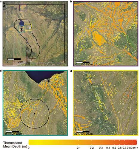
Overall, we found that thermokarst features covered 7 percent of the landscape, or 5.7 km², with considerable variability depending on slope and glacial history (Figure 2). The dendritic pattern of water tracks was found across large swaths of the low-angle hillslopes at the site. Small thermokarst pits occurred in clumps, most frequently along the inner EML moraine (Thorson 1986). Additionally, thermokarst features were evident along paths of human disturbance, including roads and dogsled/ATV tracks. Across all thermokarst shapes, the average feature size was 25 m². The deepest thermokarst feature had a maximum depth of 3.6 m. Across the site, thermokarst features averaged 0.07 m deep at their deepest point and had an average depth of 0.03 m. Erosion seemed to play a minor role in thermokarst formation because the slopes with high thermokarst activity were shallow (3°–10°) and exposure of mineral soils or disturbance to plants was only observed in recently inundated thermokarst pits.

Figure 2. (a) The mean depth of thermokarst features (2017–2019) across the study extent (9 × 9 km black box). The EML watershed is outlined in black with the EC tower and approximate tower footprint shown as a point within a circle. The three gray points show the location of the three experimental blocks at CiPEHR. Colored squares indicate insets shown in (b)–(d). (b) The largest thermokarst pond we identified in one of the most heavily thermokarst affected areas within the study extent. In addition to naturally formed features, dogsled/ATV tracks are visible throughout the area. Twenty-six percent of the inset was classified as thermokarst. (c) Thaw ponds and water tracks that drain into EML surrounding the EC tower. Nineteen percent of the inset was classified as thermokarst. (d) Extensive small thermokarst pits on the terminal moraine east of EML (the greener, shrubby area), dogsled/ATV tracks, and thermokarst pits caused by soil warming at CiPEHR. Eleven percent of the inset was classified as thermokarst.

Across the entire study area, we observed subsidence (2017–2019) of 0.03 m in non-thermokarst areas (p < .0001) and 0.02 m in thermokarst margins (p = .066) but subsidence of 0.01 m in thermokarst centers was not significant (p = .33). The rate of subsidence did not differ statistically between any of the thermokarst classes (Figure S1). Using our GPS data at CiPEHR over the same time frame, we observed subsidence across all thermokarst classes, with thermokarst centers and thermokarst margins subsiding more quickly (0.05 m) than non-thermokarst areas (0.01 m, p < .0001). The magnitude of LiDAR-derived subsidence at CiPEHR was 0.01 to 0.02 m smaller than the GPS-derived subsidence (p < .0001) but showed the same patterns across classes.

We found that thermokarst morphology varied by both feature size and shape (Figures 3 and S2). Small features were the most prevalent (51 percent), and prevalence declined exponentially as size increased. The largest class, 100,000 m² to 1 km², had a total of only nine features (0.001 percent). For shape, the most compact features, which tended to be small thermokarst pits and ponds, were most prevalent (52 percent), and the least compact features, which tended to be extensive water tracks, were the least prevalent (1 percent). Thermokarst percent cover showed very different patterns than prevalence across size and shape classes. Mid-sized thermokarst features (1,000–10,000 m²) had the greatest extent (2 percent), and both larger and smaller features were less common. For shape, percent cover showed a pattern of exponential decay from the least compact features (5 percent) to the most compact features (0.1 percent). Percent volume of thermokarst features showed patterns similar to, but more pronounced than, those for percent cover. Relatively large features (1,000–10,000 m² and 10,000–100,000 m²) had the highest percent volume (38 percent each), whereas smaller and larger features had lower percent volume. For shape, the least compact features had the highest percent cover by far (85 percent) and percent volume dropped exponentially, such that the most compact shape class accounted for very little of the thermokarst volume (<1 percent). Mean depth of thermokarst features varied considerably by size class but very little by shape. Thermokarst feature classes smaller than 1,000 m² all had a mean depth of less than 0.05 m, whereas thermokarst feature classes between 1,000 m² and 1 km² all had mean depths near or greater than 0.15 m. In contrast, all thermokarst shape classes had a mean depth around or below 0.05 m, with only a slight tendency toward shallower features at shapes in between the two extremes.

Figure 3. (a, b) Prevalence (percentage of features by count); (c), (d) percent cover (percent cover of thermokarst within that class relative to the entire study area − the sum of the classes is overall percent cover of 7 percent); (e), (f) percent volume; (g), (h) mean depth of thermokarst features by size and shape class. Labels in (a) and (b) indicate the number of features within each class.

EML decadal change

Within the EML watershed, we found a higher degree of thermokarst impact than across the study area as a whole. Within the watershed, 12 percent, or 1.3 km², of the landscape was impacted by thermokarst, compared to 7 percent within the larger study area and exactly the same as in 2008. Much of the watershed was covered by water tracks and a small stream feeding into EML, which was likely responsible for the elevated thermokarst percent cover relative to the rest of the study area. Additionally, the watershed has a higher ratio of road miles to area than the rest of the study area and the road is flanked by thermokarst features for nearly its entire length. Finally, there are more dogsled/ATV tracks in the vicinity of the lake and road than in other regions of the study area, although these features cover much less area than water tracks.

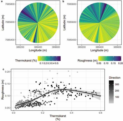
Thermokarst percent cover and roughness varied considerably across the EC tower footprint, with higher thermokarst percent cover and roughness occurring north and northwest of the tower (Figure 4). This trend was driven by a system of deeply incised water tracks primarily in the north and northwest regions of the EC tower fetch and a patch of small thermokarst features in the northeast region of the fetch (Figures 2c and S3). There was a nonlinear relationship between surface roughness and thermokarst. Surface roughness increased with increasing thermokarst to about 30 percent cover and then declined somewhat with greater thermokarst percent cover. Since 2008, we found that average microtopography in the entire EC tower footprint increased by 1.62 cm (Belshe et al. 2012), which may indicate that the landscape is subsiding more quickly than older thermokarst features.

Figure 4. (a) Thermokarst percent cover in 1° increments at the EC tower, (b) surface roughness in 1° increments at the EC tower, and (c) the relationship between percentage thermokarst cover and surface roughness at the EC tower, with the grayscale indicating the direction from which the measurement came (relative to the tower).

Response of CO₂ fluxes to abrupt thaw

Abrupt thaw drove higher CO₂ release (Figure S4), with thermokarst percent cover being a strong predictor of all CO₂ fluxes (NEE, GPP, R_eco), particularly during the GS day (Figure 5). All selected models included thermokarst percent cover, month, and the interaction between the two. Thermokarst percent cover explained more variation in GPP (r² = 0.56) and R_eco (GS day: r² = 0.49; NGS/night: r² = 0.24) than in NEE (GS day: r² = 0.39; NGS/night: r² = 0.22). During the GS day, GPP and R_eco increased with thermokarst percent cover, with the response peaking during the growing season. During the NGS/night, there was a noticeable seasonal trend in the relationship between thermokarst percent cover and R_eco, with very little impact of thermokarst on R_eco during the winter and early spring and stimulation of R_eco by thermokarst during the GS and early fall, particularly August and October. During the GS day, abrupt thaw stimulated GPP more than R_eco, resulting in higher carbon uptake, particularly during peak growing season in July. During the NGS/night, however, abrupt thaw stimulated carbon release in all months except February. In February, the relatively strong stimulation of the CO₂ sink by thermokarst appears to be confounded by wind speed and wind direction. This was because winter storms, which release CO₂ trapped in snow or cracks in the soil, primarily came from the southwest, which happens to have low thermokarst percent cover. On an annual scale, the impact of abrupt thaw on R_eco was stronger than the impact on GPP, resulting in greater CO₂ release (Figure S4).

Figure 5. Coefficients for the linear regressions of GPP, NEE, and R_eco by thermokarst percent cover. Positive intercepts indicate a source when no thermokarst is present and negative intercepts indicate a sink when no thermokarst is present. Positive slopes indicate that fluxes trend toward a larger source or smaller sink as thermokarst percent cover increases, depending on the sign of the flux. Negative slopes indicate that fluxes trend toward a smaller source or larger sink as thermokarst percent cover increases.

Response of CH₄ fluxes to abrupt thaw

Abrupt thaw was a significant, but small, predictor of CH₄ fluxes, with the strongest relationship occurring during the growing season and fall (Figure 6; r² = 0.071). For all months except January and February we found that CH₄ release increased with thermokarst percent cover, with the strongest relationships between June and October and weaker relationships in the winter and early spring. In contrast, in January and February, CH₄ release was exceptionally high at low thermokarst percent cover, which was largely due to high wind speed during storms coming from directions with low thermokarst percent cover, likely releasing CH₄ trapped in snow. During the GS day, CH₄ pulse release showed some evidence of being influenced by thermokarst percent cover, because higher release tended to occur from areas of higher thermokarst percent cover (Figure S5), but soil moisture had a stronger influence on CH₄ pulse release. During the NGS, wind speed had a strong influence on CH₄ pulse release and thermokarst percent cover did not appear to play a strong role.

Figure 6. Coefficients for the linear regression of non-pulse CH₄ fluxes by thermokarst percent cover and month. Positive values for intercepts indicate a source when no thermokarst is present and negative values for intercepts indicate a sink when no thermokarst is present. Positive values for slopes indicate that fluxes trend toward a larger source or smaller sink as thermokarst percent cover increases, depending on the sign of the flux. Negative values for slopes indicate that fluxes trend toward a smaller source or larger sink as thermokarst percent cover increases.

Discussion

Thermokarst morphology and impact on carbon fluxes

We found that at least 7 percent of the site was impacted by thermokarst and, based on a qualitative assessment of thermokarst morphology, the impact of these features on carbon thaw and flux varied by thermokarst size and shape (Figure 3). Small thermokarst pits, most common on the inner EML moraine and previously glaciated low-angle slopes to the east of the moraine, were by far the most numerous thermokarst features. Given the glacial history of these areas, these features could be the result of the thaw of buried glacial ice (Thorson 1986; Harris and Murton 2005) and the presence of glacial till (Osterkamp et al. 2009). By area, a much smaller number of larger, less compact features accounted for the vast majority of thermokarst-impacted land. These features tended to be extensive systems of water tracks, which were longer and deeper than the smaller pits. Because of this, these features had an outsized impact on the ecosystem by thawing more permafrost and the carbon it contains. At this site, we previously found that subsidence associated with abrupt thaw can thaw carbon at twice the rate expected from that of gradual thaw alone (Rodenhizer et al. 2020). With 7 percent of the landscape currently undergoing abrupt thaw, this could mean that, at the landscape level, permafrost carbon is thawing 7 percent faster than increases in active layer thickness indicate. It is important to note, however, that this rate will change as thaw progresses into deeper soils with lower carbon content.

Thermokarst percent cover, in combination with month, explained between 22 and 56 percent of GPP, R_eco, and NEE, indicating that it captures some of the long-term variability associated with a wide variety of environmental predictors of carbon fluxes, although it only explained 7 percent of CH₄ flux (Figure 5). Given that carbon fluxes respond to many environmental variables in complex ways, the high r² values in our linear models indicated that thermokarst was a proxy variable for several environmental variables, with the ability to explain ~50 percent of GS day GPP and R_eco when month is also considered. Because thermokarst typically occurs over the course of years to decades, it may be a proxy for environmental variables such as deep soil temperature, talik formation, and nutrient availability, which exert slower, long-term control on fluxes than environmental variables like light level or air temperature, which can change drastically throughout the course of a day (Lee, Schuur, and Vogel 2010; Lee et al. 2011; Belshe et al. 2012).

Net carbon dioxide release was promoted by abrupt thaw at this site (Figure S4). Changes in NEE depend on the balance between GPP and R_eco, both of which can shift in divergent directions in response to abrupt thaw. Although we found that plant growth was promoted within thermokarst features during the growing season daytime, resulting in higher annual GPP, it was not sufficient to offset higher R_eco at night and during the nongrowing season (Figures S4, Figure 5). This reinforces the idea that winter respiration rates have a very important role in determining annual CO₂ balance across the northern permafrost region (Natali et al. 2019; Watts et al. 2021). This site is already a CO₂ source in most years (Plaza et al. 2019; T. Schuur et al. 2021) because of the combined impacts of gradual and abrupt thaw. Our findings isolated the response of CO₂ flux to abrupt thaw and indicate that this site is likely to become an even stronger CO₂ source as abrupt thaw expands. Higher NEE (more release of CO₂) from thermokarst features has also been found in previous studies at EML (Vogel et al. 2009; Trucco et al. 2012) and elsewhere (Cassidy, Christen, and Henry 2016; Euskirchen et al. 2017) and in modeling studies (Parazoo et al. 2018; Turetsky et al. 2020), supporting our results. However, the opposite pattern (lower NEE) has also been documented at EML (Lee et al. 2011) and elsewhere (Euskirchen et al. 2014; Wickland et al. 2020). The varied net CO₂ response of thermokarst features across sites is likely due in part to thermokarst morphology, which regulates environmental conditions such as soil temperature (Lee et al. 2011; Mauritz et al. 2017), soil moisture (Euskirchen et al. 2017; Mauritz et al. 2017; Rodenhizer et al. 2020), and rates of erosion (Abbott and Jones 2015). Because these changes in environmental conditions can result in either increases or decreases in GPP and/or R_eco, the overall effect on NEE is highly variable, and the opposite responses observed across sites and through time are not unexpected. Despite the wide variability of NEE response to abrupt thaw, the balance of the evidence suggests that the ability of abrupt thaw to rapidly thaw permafrost carbon results in substantial release of carbon that was previously stored in permafrost soils.

Abrupt thaw promoted higher GPP during the growing season (Figure 5), because highly vegetated water tracks were the most extensive form of thermokarst. Although we have previously observed die-off of plants in young, recently inundated thermokarst features at this site (Rodenhizer et al. 2020; Taylor et al. 2021), GPP was stimulated by abrupt thaw in the current study, likely due to the response of extensive (and typically older) water tracks (Curasi, Loranty, and Natali 2016). Higher GPP in water tracks at this site was likely due to warmer soil temperatures (Lee et al. 2011), the release of nutrients from the deepening thaw front (Salmon et al. 2016; Hewitt et al. 2018, 2019), and low rates of erosion allowing the establishment of wet-adapted plants (Jorgenson and Osterkamp 2005). Because this site is relatively wet, we do not believe that the alleviation of drought in thermokarst features played a strong role in increasing GPP, as was observed in Euskirchen et al. (2017). Because water tracks are the most widespread thermokarst morphology at our site, this site is likely seeing an overall increase in photosynthesis and vegetation biomass as abrupt thaw progresses.

Abrupt thaw promoted R_eco year-round (Figure 5), outpacing increases in GPP and resulting in the loss of old permafrost carbon (Figure S4). Increases in R_eco were due partially to higher root respiration associated with higher plant growth in water tracks (Lee, Schuur, and Vogel 2010; Hicks Pries et al. 2013, 2015, 2016). However, increasing year-round heterotrophic respiration must be responsible for the overall shift to higher net carbon release, despite its smaller magnitude. This is because carbon release through autotrophic respiration offsets only about half of carbon uptake through photosynthesis (Collalti, Prentice, and Polle 2019). The increase in heterotrophic respiration is likely due to higher availability of carbon as a microbial energy source, increasing soil temperatures, and the presence of taliks, which provide unfrozen soil conditions year-round (Natali et al. 2019; Pegoraro et al. 2020). Although erosion can limit R_eco through the rapid export of permafrost carbon (Abbott and Jones 2015), this did not appear to play a noticeable role due to the low rates of erosion at this site. Because this site is relatively wet and prone to anaerobic conditions (which can protect soil carbon from mineralization), the increase in heterotrophic respiration has previously been shown to be particularly strong during dry years when waterlogging is alleviated (Pegoraro et al. 2020). Some of the carbon being respired from thermokarst has likely been stored in permafrost for hundreds to thousands of years (Hicks Pries, Schuur, and Crummer 2013; Pegoraro et al. 2019, 2020), particularly as the thaw front deepens rapidly into layers of older carbon.

Abrupt thaw promoted higher CH₄ release nearly year-round (Figure 6), likely due to anoxic conditions in waterlogged soils and longer periods of unfrozen conditions in thermokarst (Taylor et al. 2018, 2021). Unlike the varied responses of NEE to thermokarst, there is high agreement in the literature that CH₄ release is promoted by abrupt thaw (Kutzbach, Wagner, and Pfeiffer 2004; Nauta et al. 2015; Lindgren et al. 2016; Cooper et al. 2017; Burke et al. 2019; Wickland et al. 2020). We found that the stimulation of CH₄ release by abrupt thaw was strongest between spring thaw and early winter. Although CH₄ production occurs in taliks throughout the winter, it is often trapped by snow cover until spring thaw, explaining the strong response of CH₄ flux to abrupt thaw that we observed in March through May (Tokida et al. 2007; Song et al. 2012; Tagesson et al. 2012; Pirk et al. 2017; Raz-Yaseef et al. 2017; Taylor et al. 2018). Additionally, warmer soil temperatures and the presence of taliks in thermokarst features promote more rapid and deeper thaw throughout the growing season (E. A. G. Schuur et al. 2007). Combined with higher soil moisture increasing the likelihood of anoxic conditions in thermokarst depressions (E. A. G. Schuur et al. 2007), this provides conditions prone to CH₄ production (Taylor et al. 2018). During the early winter, an increase in the length of the zero curtain (the time during freeze-up when soils are unfrozen but near 0°C), particularly in thermokarst features, could be allowing methanogenesis to continue later into the nongrowing season (Zona et al. 2016; Arndt et al. 2019; Bao et al. 2021). The increase in CH₄ release has the potential to shift the radiative forcing of the site significantly, even though CH₄ fluxes are much smaller than CO₂ fluxes. Methane is a forty-five times more powerful greenhouse gas than CO₂ over 100 years (Myhre, Shindell, and Pongratz 2014; Neubauer and Megonigal 2015), meaning that a small shift from CO₂ production to CH₄ production under wet soil conditions can have a large impact on the radiative forcing of carbon emissions. Because CH₄ is responsible for 61 percent of the radiative forcing due to carbon emissions at this site (Taylor et al. 2018), the stimulation of CH₄ release by abrupt thaw is likely to have a large impact on the radiative forcing of the site, despite the smaller magnitude of fluxes and weaker relationship. Overall, we found that ecological changes associated with abrupt permafrost thaw are playing an important long-term role in exacerbating net carbon release, even as GPP increases.

Subsidence and thermokarst development through time

Across the study site, we saw evidence of expansion and initiation of thermokarst, rather than deepening of established features. Greater extent of thermokarst resulted in lower surface roughness and could indicate that hydraulic connectivity is slowly increasing at the site, as thermokarst features expand and taliks interlink (Devoie et al. 2019). This could eventually result in better drainage and drier surface soils (Teufel and Sushama 2019). We draw on three lines of reasoning to support the conclusion that the extent of abrupt thaw is increasing, which are outlined here and described in detail in the following paragraphs. First, across the site, subsidence occurred most rapidly in areas not classified as thermokarst and old thermokarst features did not subside noticeably. However, small, recently initiated thermokarst features (approximately one decade old or less) within CiPEHR subsided rapidly. Second, aerial imagery dating to 1954 and anecdotal evidence at the site indicate the initiation of thaw pits and the expansion of water tracks upslope through time. Additionally, the observed lack of change in thermokarst extent between Belshe, Schuur, and Grosse (2013) and the current study is explained by differences in methodology resulting in the current study being more conservative in the classification of thermokarst. Third, a slight increase in microtopography from Belshe et al. (2012), despite widespread subsidence, is consistent with the initiation of new thermokarst features and the expansion, but not deepening, of old thermokarst features.

Across the study site, the lack of subsidence in thermokarst centers between 2017 and 2019 indicated that preexisting thermokarst features did not deepen significantly, and the highest rate of subsidence in non-thermokarst areas indicated that there may be thermokarst initiation and expansion occurring (Figure S1). The lack of subsidence in thermokarst centers across the site may indicate that these older features have already thawed near-surface permafrost with the highest ice content and reached a more stable depth (French and Shur 2010). This supports the idea that older thermokarst features were primarily expanding rather than deepening. In addition, new features may have formed across the landscape, contributing to the higher rate of subsidence in non-thermokarst areas. Though these areas have not yet subsided sufficiently for thermokarst features to be detectable, the ubiquitous nature of abrupt thaw across the site, the rate of thaw (~1 cm year⁻¹), and the high, but variable (25–78 percent by mass), ice content at the site indicate that this is not gradual thaw but initiation of abrupt thaw (Rodenhizer et al. 2020). At CiPEHR, however, the rates of subsidence indicate that they were both deepening and expanding, because thermokarst features were initiated recently (experimental warming started in 2008) and were still actively forming (Osterkamp et al. 2009). Our inability to statistically distinguish the rate of subsidence between thermokarst classes using LiDAR data may be partially due to the opposite responses of thermokarst features of different ages and partially a consequence of insufficient image resolution to precisely distinguish thermokarst margins.

Documenting change in thermokarst over a decade was a challenge because methodological differences resulted in a more conservative classification than in Belshe, Schuur, and Grosse (2013). There is evidence of thermokarst expansion at the site from aerial photography dating back to 1954 in tandem with both rising air and permafrost temperatures (Osterkamp et al. 2009). On the ground more recently, we have documented increases in active layer thickness and subsidence of over 1 cm year⁻¹ (Rodenhizer et al. 2020) and seen the expansion of water tracks (necessitating the relocation of the EC tower). Additionally, our classification indicated that water tracks extended farther upslope than in 2008, and we found a larger number of small features that could indicate thermokarst expansion and initiation. However, this was counterbalanced by a larger number of non-thermokarst cells within thermokarst features in the overall extent, which seems to be due primarily to differences in the theoretical approach to thermokarst classification. Belshe, Schuur, and Grosse (2013) used spectral data to classify thermokarst based primarily on the visible changes to vegetation associated with thermokarst. This means that the presence of thicker, greener vegetation in water tracks (Curasi, Loranty, and Natali 2016) resulted in a thermokarst classification with fewer gaps in their study. In our study, on the other hand, areas within a thermokarst feature would be classified as non-thermokarst if their elevation was even slightly higher than the surrounding landscape, despite increased vegetation productivity that would indicate the location is undergoing abrupt thaw. Though resolution must also play some role in the different distributions of thermokarst between the two studies, we were able to confirm that resolution did not impact the overall extent by finding very little change in thermokarst extent when we resampled our classification to 3-m resolution (as in Belshe, Schuur, and Grosse 2013). Taken together, all of this leads us to conclude that our thermokarst classification is more conservative than that of Belshe, Schuur, and Grosse (2013) and that thermokarst percentage cover within the EML watershed has likely exceeded 12 percent (as found in both studies) in the past decade.

The slight increase in microtopography since 2008 could also be an indication of the increasing extent of thermokarst with limited deepening of older features (Figure S3). As thermokarst features have expanded and the landscape as a whole has subsided, the average landscape elevation has decreased, and thermokarst features may no longer have been subsiding where ground ice had already thawed (Figure S1). Because microtopography was calculated as the average neighborhood elevation subtracted from the local elevation, a decrease in average elevation necessarily results in an increase in microtopography for cells that subsided more slowly than the landscape average. Therefore, we conclude that the slight increase in microtopography was an indication of the increasing ubiquity of thermokarst at the site.

Discussion of validation and utility

The thermokarst detection algorithm presents a unique opportunity for the detection of thermokarst anywhere a single ground elevation map is available, rather than relying on change detection from two or more elevation maps at different time points. Removing the necessity of repeat imagery to identify thermokarst means that this method could be applied to a broader range of sites than is otherwise possible, because airborne LiDAR availability is limited and satellite imagery does not achieve the necessary spatial resolution (Kääb 2008; Westermann et al. 2015). However, applying the analysis on multiple DTMs and combining the classifications into one result, as we did, can help alleviate errors. Additionally, it may be possible to scale this method to larger regions as access to elevation data improves. Unfortunately, the ArcticDEM (Porter et al. 2018) is not suitable for detecting many types of thermokarst features, because it uses the elevation of the vegetation canopy rather than the ground surface. It could, however, potentially be used to detect features with high levels of erosion or inundation that have limited vegetation or features that are deeper than the tallest vegetation. This would build upon our current understanding of the distribution of thermokarst, because circumpolar studies of thermokarst have not yet mapped discrete features. There are, however, some limitations to the thermokarst detection algorithm. First, a high-resolution elevation data set is required, because poor resolution could lead to the detection of larger landscape features, like valleys, rather than thermokarst, as in the case of the similar topographic position index (De Reu et al. 2013). In this study, we used elevation at 1-m resolution. We expect it would be possible to use up to 10-m resolution data to detect large features, based on the fact that thermokarst features 100 m² or smaller covered only ~1.5 percent of our site (Figure 3). These larger features were responsible for the vast majority of permafrost thaw, indicating that they may play a larger role in carbon dynamics, despite the prevalence of small thermokarst pits. Second, the necessity of high-resolution data requires more processing power than is readily available at this point, although Google Earth Engine could alleviate this issue. Despite these limitations, the increasing availability of high-resolution elevation data across the circumpolar region means that this method can be applied across an increasingly broad range and shows promise for improving our understanding of the distribution and extent of thermokarst across the Arctic.

Conclusion

Abrupt thaw is contributing to carbon release above that caused by gradual thaw at EML. At least 7 percent of the site as a whole and at least 12 percent of the EML watershed is undergoing abrupt thaw, with evidence of new thermokarst initiation and expansion driving abrupt thaw processes rather than deepening of older thermokarst features. We identified a large number of small, relatively shallow thermokarst pits, but deeper and larger water tracks were more extensive and were responsible for thawing more permafrost than small features. There was strong evidence that abrupt thaw correlated with increases in both GPP and R_eco, but because R_eco responded more strongly to thaw, the net result was higher CO₂ release. This is likely due to the high percent cover of water tracks, which tend to have much thicker vegetation, enhancing photosynthesis during the GS and ecosystem respiration both during and outside the GS. Additionally, abrupt thaw accelerated the release of CH₄ in nearly all months, which is responsible for about 61 percent of the greenhouse gas radiative forcing of the site (Taylor et al. 2018). As the climate continues to warm, thermokarst features will expand to cover more of the landscape, thaw more permafrost carbon, and push more permafrost ecosystems toward becoming carbon sources for the first time in thousands of years. With many modeling studies and field studies, including this one, indicating that abrupt thaw could increase carbon release significantly, it is imperative to understand where abrupt thaw is occurring and to work to include abrupt thaw processes in Earth System Models.

Acknowledgments

This study made use of imagery that was collected as part of the Arctic–Boreal Vulnerability Experiment. Resources supporting this work were provided by the NASA High-End Computing Program through the NASA Center for Climate Simulation at Goddard Space Flight Center. Particular thanks to Elizabeth Hoy and Tristan Goulden for their help with ABoVE and NEON data sets.

Disclosure statement

No potential conflict of interest was reported by the authors.

Supplementary material

Supplemental data for this article can be accessed online at https://doi.org/10.1080/15230430.2022.2118639

Additional information

Funding

This work was supported by the National Science Foundation (NSF) Navigating the New Arctic: Long Term Research in Environmental Biology: The Arctic Carbon and Climate (ACCLIMATE) Observatory: Tundra Ecosystem Carbon Balance and Old Carbon Loss as a Consequence of Permafrost Degradation (Award No. 1754839). Supplemental funding was provided by the Bonanza Creek LTER, a partnership between the University of Alaska Fairbanks and the U.S. Forest Service. Significant funding for collection of these data was provided by the National Science Foundation Long-Term Ecological Research program (NSF Grant Nos. DEB-1636476, DEB-1026415, DEB-0620579, DEB-0423442, DEB-0080609, DEB-9810217, DEB-9211769, DEB-8702629) and by the U.S. Forest Service, Pacific Northwest Research Station (Agreement No. RJVA-PNW-01-JV-11261952-231).

References

- Abbott, B. W., and J. B. Jones. 2015. Permafrost collapse alters soil carbon stocks, respiration, CH4, and N2O in upland tundra. Global Change Biology 21 (12):4570–87. doi:10.1111/gcb.13069.
- Abe, T., G. Iwahana, P. V. Efremov, A. R. Desyatkin, T. Kawamura, A. Fedorov, Y. Zhegusov, K. Yanagiya, and T. Tadono. 2020. Surface displacement revealed by L-band InSAR analysis in the Mayya area, Central Yakutia, underlain by continuous permafrost. Earth, Planets and Space 72 (1):138. doi:10.1186/s40623-020-01266-3.
- Arndt, K. A., W. C. Oechel, J. P. Goodrich, B. A. Bailey, A. Kalhori, J. Hashemi, C. Sweeney, and D. Zona. 2019. Sensitivity of methane emissions to later soil freezing in Arctic tundra ecosystems. Journal of Geophysical Research: Biogeosciences 124 (8):2595–609. doi:10.1029/2019JG005242.
- Bao, T., X. Xu, G. Jia, D. P. Billesbach, and R. C. Sullivan. 2021. Much stronger tundra methane emissions during autumn freeze than spring thaw. Global Change Biology 27 (2):376–87. doi:10.1111/gcb.15421.
- Belshe, E. F., E. A. G. Schuur, B. M. Bolker, and R. Bracho. 2012. Incorporating spatial heterogeneity created by permafrost thaw into a landscape carbon estimate. Journal of Geophysical Research: Biogeosciences 117 (G1). doi:10.1029/2011JG001836.
- Belshe, E. F., E. A. G. Schuur, and G. Grosse. 2013. Quantification of upland thermokarst features with high resolution remote sensing. Environmental Research Letters 8 (3):35016. doi:10.1088/1748-9326/8/3/035016.
- Burke, S. A., M. Wik, A. Lang, A. R. Contosta, M. Palace, P. M. Crill, and R. K. Varner. 2019. Long‐term measurements of methane ebullition from thaw ponds. Journal of Geophysical Research: Biogeosciences 124 (7):2208–21. doi:10.1029/2018JG004786.
- Campitelli, E. 2021. Ggnewscale: Multiple fill and colour scales in “ggplot2” (0.4.5) [R]. https://CRAN.R-project.org/package=ggnewscale.
- Cassidy, A. E., A. Christen, and G. H. R. Henry. 2016. The effect of a permafrost disturbance on growing-season carbon-dioxide fluxes in a high Arctic tundra ecosystem. Biogeosciences 13 (8):2291–303. doi:10.5194/bg-13-2291-2016.
- Clayden, J. 2020. Mmand: Mathematical morphology in any number of dimensions (1.6.1) [R]. https://CRAN.R-project.org/package=mmand.
- Collalti, A., I. C. Prentice, and A. Polle. 2019. Is NPP proportional to GPP? Waring’s hypothesis 20 years on. Tree Physiology 39 (8):1473–83. doi:10.1093/treephys/tpz034.
- Congalton, R. G., and K. Green. 2019. Assessing the accuracy of remotely sensed data: Principles and practices. 3rd ed. Boca Raton, FL: CRC Press.
- Cooper, M. D. A., C. Estop-Aragonés, J. P. Fisher, A. Thierry, M. H. Garnett, D. J. Charman, J. B. Murton, G. K. Phoenix, R. Treharne, S. V. Kokelj, et al. 2017. Limited contribution of permafrost carbon to methane release from thawing peatlands. Nature Climate Change 7 (7):507–11. doi:10.1038/nclimate3328.
- Curasi, S. R., M. M. Loranty, and S. M. Natali. 2016. Water track distribution and effects on carbon dioxide flux in an eastern Siberian upland tundra landscape. Environmental Research Letters 11 (4):45002. doi:10.1088/1748-9326/11/4/045002.
- Delwiche, K. B., S. H. Knox, A. Malhotra, E. Fluet-Chouinard, G. McNicol, S. Feron, Z. Ouyang, D. Papale, C. Trotta, E. Canfora, et al. 2021. FLUXNET-CH4: A global, multi-ecosystem dataset and analysis of methane seasonality from freshwater wetlands. Preprint. Biosphere – Biogeosciences. doi:10.5194/essd-2020-307.
- De Reu, J., J. Bourgeois, M. Bats, A. Zwertvaegher, V. Gelorini, P. De Smedt, W. Chu, M. Antrop, P. De Maeyer, P. Finke, et al. 2013. Application of the topographic position index to heterogeneous landscapes. Geomorphology 186:39–49. doi:10.1016/j.geomorph.2012.12.015.
- Devoie, É. G., J. R. Craig, R. F. Connon, and W. L. Quinton. 2019. Taliks: A tipping point in discontinuous permafrost degradation in peatlands. Water Resources Research 55 (11):9838–57. doi:10.1029/2018WR024488.
- Dowle, M., and A. Srinivasan. 2021. Data.table: Extension of `data.frame`. (1.14.0) [R]. https://CRAN.R-project.org/package=data.table.
- Euskirchen, E. S., C. W. Edgar, M. Syndonia Bret-Harte, A. Kade, N. Zimov, and S. Zimov. 2017. Interannual and seasonal patterns of carbon dioxide, water, and energy fluxes from ecotonal and thermokarst-impacted ecosystems on carbon-rich permafrost soils in northeastern Siberia. Journal of Geophysical Research: Biogeosciences 122 (10):2651–68. doi:10.1002/2017JG004070.
- Euskirchen, E. S., C. W. Edgar, M. R. Turetsky, M. P. Waldrop, and J. W. Harden. 2014. Differential response of carbon fluxes to climate in three peatland ecosystems that vary in the presence and stability of permafrost: Carbon fluxes and permafrost thaw. Journal of Geophysical Research: Biogeosciences 119 (8):1576–95. doi:10.1002/2014JG002683.
- Farquharson, L. M., V. E. Romanovsky, W. L. Cable, D. A. Walker, S. V. Kokelj, and D. Nicolsky. 2019. Climate change drives widespread and rapid thermokarst development in very cold permafrost in the Canadian High Arctic. Geophysical Research Letters 46 (12):6681–89. doi:10.1029/2019GL082187.
- French, H., and Y. Shur. 2010. The principles of cryostratigraphy. Earth-Science Reviews 101 (3–4):190–206. doi:10.1016/j.earscirev.2010.04.002.
- Garnier, S., N. Ross, R. Rudis, M. Sciaini, and C. Scherer. 2021. Rvision—Colorblind-friendly color maps for R (0.6.1) [R]. https://cran.r-project.org/web/packages/viridis/index.html.
- Grosse, G., V. E. Romanovsky, K. Walter, A. Morgenstern, H. Lantuit, annd S. Zimov. 2008. Distribution of thermokarst lakes and ponds at three yedoma sites in siberia. In Ninth International Conference on Permafrost, ed. D. L. Kane and K. M. Hinkel. Fairbanks, AK: Institute of Northern Engineering, University of Alaska Fairbanks, 551–556.
- Grosse, G., L. Schirrmeister, and T. J. Malthus. 2006. Application of Landsat-7 satellite data and a DEM for the quantification of thermokarst-affected terrain types in the periglacial Lena–Anabar coastal lowland. Polar Research 25 (1):51–67. doi:10.1111/j.1751-8369.2006.tb00150.x.
- Harris, C., and J. B. Murton. 2005. Interactions between glaciers and permafrost: An introduction. Geological Society, London, Special Publications 242 (1):1–9. doi:10.1144/GSL.SP.2005.242.01.01.
- Hewitt, R. E., M. R. DeVan, I. V. Lagutina, H. Genet, A. D. McGuire, D. L. Taylor, and M. C. Mack. 2019. Mycobiont contribution to tundra plant acquisition of permafrost‐derived nitrogen. New Phytologist 226 (1): 126–141. doi:10.1111/nph.16235.
- Hewitt, R. E., D. L. Taylor, H. Genet, A. D. McGuire, and C. Mack. 2018. Below‐ground plant traits influence tundra plant acquisition of newly thawed permafrost nitrogen. Journal of Ecology 107 (2):950–962. doi:10.1111/1365-2745.13062.
- Hicks Pries, C. E., E. A. G. Schuur, and K. G. Crummer. 2013. Thawing permafrost increases old soil and autotrophic respiration in tundra: Partitioning ecosystem respiration using δ13C and ∆14C. Global Change Biology 19 (2):649–61. doi:10.1111/gcb.12058.
- Hicks Pries, C. E., E. A. G. Schuur, S. M. Natali, and K. G. Crummer. 2016. Old soil carbon losses increase with ecosystem respiration in experimentally thawed tundra. Nature Climate Change 6 (2):214–18. doi:10.1038/nclimate2830.
- Hicks Pries, C. E., E. A. G. Schuur, J. G. Vogel, and S. M. Natali. 2013. Moisture drives surface decomposition in thawing tundra. Journal of Geophysical Research: Biogeosciences 118 (3):1133–43. doi:10.1002/jgrg.20089.
- Hicks Pries, C. E., R. S. P. van Logtestijn, E. A. G. Schuur, S. M. Natali, J. H. C. Cornelissen, R. Aerts, and E. Dorrepaal. 2015. Decadal warming causes a consistent and persistent shift from heterotrophic to autotrophic respiration in contrasting permafrost ecosystems. Global Change Biology 21 (12):4508–19. doi:10.1111/gcb.13032.
- Hijmans, R. J. 2021. Raster: Geographic data analysis and modeling (3.4-10) [R]. https://CRAN.R-project.org/package=raster.
- Hinkel, K. M., and F. E. Nelson. 2003. Spatial and temporal patterns of active layer thickness at Circumpolar Active Layer Monitoring (CALM) sites in northern Alaska, 1995–2000. Journal of Geophysical Research 108 (D2):8168. doi:10.1029/2001JD000927.
- Houghton, R. A. 2007. Balancing the global carbon budget. Annual Review of Earth and Planetary Sciences 35 (1):313–47. doi:10.1146/annurev.earth.35.031306.140057.
- Jensen, A. E., K. A. Lohse, B. T. Crosby, and C. I. Mora. 2014. Variations in soil carbon dioxide efflux across a thaw slump chronosequence in northwestern Alaska. Environmental Research Letters 9 (2):25001. doi:10.1088/1748-9326/9/2/025001.
- Jones, B. M., G. Grosse, C. D. Arp, E. Miller, L. Liu, D. J. Hayes, and C. F. Larsen. 2015. Recent Arctic tundra fire initiates widespread thermokarst development. Scientific Reports 5 (1):15865. doi:10.1038/srep15865.
- Jones, B. M., J. M. Stoker, A. E. Gibbs, G. Grosse, V. E. Romanovsky, T. A. Douglas, N. E. M. Kinsman, and B. M. Richmond. 2013. Quantifying landscape change in an Arctic coastal lowland using repeat airborne LiDAR. Environmental Research Letters 8 (4):45025. doi:10.1088/1748-9326/8/4/045025
- Jorgenson, M. T., T. A. Douglas, A. K. Liljedahl, J. E. Roth, T. C. Cater, W. A. Davis, G. V. Frost, P. F. Miller, and C. H. Racine. 2020. The roles of climate extremes, ecological succession, and hydrology in repeated permafrost aggradation and degradation in fens on the Tanana Flats, Alaska. Journal of Geophysical Research: Biogeosciences 125 (12). doi: 10.1029/2020JG005824.
- Jorgenson, M. T., and T. E. Osterkamp. 2005. Response of boreal ecosystems to varying modes of permafrost degradation. Canadian Journal of Forest Research 35 (9):2100–11. doi:10.1139/X05-153.
- Jorgenson, M. T., V. Romanovsky, J. Harden, Y. Shur, J. O’Donnell, E. A. G. Schuur, M. Kanevskiy, and S. Marchenko. 2010. Resilience and vulnerability of permafrost to climate change. Canadian Journal of Forest Research 40 (7):1219–36. doi:10.1139/X10-060.
- Jorgenson, M. T., Y. L. Shur, and E. R. Pullman. 2006. Abrupt increase in permafrost degradation in Arctic Alaska. Geophysical Research Letters 33 (2):L02503. doi:10.1029/2005GL024960.
- Kääb, A. 2008. Remote sensing of permafrost-related problems and hazards. Permafrost and Periglacial Processes 19 (2):107–36. doi:10.1002/ppp.619.
- Kanevskiy, M., Y. Shur, T. Jorgenson, D. R. N. Brown, N. Moskalenko, J. Brown, D. A. Walker, M. K. Raynolds, and M. Buchhorn. 2017. Degradation and stabilization of ice wedges: Implications for assessing risk of thermokarst in northern Alaska. Geomorphology 297:20–42. doi:10.1016/j.geomorph.2017.09.001.
- Kassambara, A. 2020. Ggpubr: “ggplot2” based publication ready plots (0.4.0) [R]. https://CRAN.R-project.org/package=ggpubr.
- Kljun, N., P. Calanca, M. W. Rotach, and H. P. Schmid. 2015. A simple two-dimensional parameterisation for Flux Footprint Prediction (FFP). Geoscientific Model Development 8 (11):3695–713. doi:10.5194/gmd-8-3695-2015.
- Kokelj, S. V., and M. T. Jorgenson. 2013. Advances in thermokarst research: Recent advances in research investigating thermokarst processes. Permafrost and Periglacial Processes 24 (2):108–19. doi:10.1002/ppp.1779.
- Kokelj, S. V., J. Kokoszka, J. van der Sluijs, A. C. A. Rudy, J. Tunnicliffe, S. Shakil, S. E. Tank, and S. Zolkos. 2021. Thaw-driven mass wasting couples slopes with downstream systems, and effects propagate through Arctic drainage networks. The Cryosphere 15 (7):3059–81. doi:10.5194/tc-15-3059-2021.
- Kutzbach, L., D. Wagner, and E.-M. Pfeiffer. 2004. Effect of microrelief and vegetation on methane emission from wet polygonal tundra, Lena Delta, Northern Siberia. Biogeochemistry 69 (3):341–62. doi:10.1023/B:BIOG.0000031053.81520.db.
- Lantz, T. C., and S. V. Kokelj. 2008. Increasing rates of retrogressive thaw slump activity in the Mackenzie Delta region, N.W.T., Canada. Geophysical Research Letters 35 (6):L06502. doi:10.1029/2007GL032433.
- Lara, M. J., H. Genet, A. D. McGuire, E. S. Euskirchen, Y. Zhang, D. R. N. Brown, M. T. Jorgenson, V. Romanovsky, A. Breen, and W. R. Bolton. 2016. Thermokarst rates intensify due to climate change and forest fragmentation in an Alaskan boreal forest lowland. Global Change Biology 22 (2):816–29. doi:10.1111/gcb.13124.
- Lee, H., E. A. G. Schuur, and J. G. Vogel. 2010. Soil CO2 production in upland tundra where permafrost is thawing. Journal of Geophysical Research 115 (G1):G01009. doi:10.1029/2008JG000906.
- Lee, H., E. A. G. Schuur, J. G. Vogel, M. Lavoie, D. Bhadra, and C. L. Staudhammer. 2011. A spatially explicit analysis to extrapolate carbon fluxes in upland tundra where permafrost is thawing. Global Change Biology 17 (3):1379–93. doi:10.1111/j.1365-2486.2010.02287.x.
- Lenth, R. V. 2021. Emmeans: Estimated marginal means, aka least-squares means (1.6.1) [R]. https://CRAN.R-project.org/package=emmeans.
- Lindgren, P. R., G. Grosse, K. M. Walter Anthony, and F. J. Meyer. 2016. Detection and spatiotemporal analysis of methane ebullition on thermokarst lake ice using high-resolution optical aerial imagery. Biogeosciences 13 (1):27–44. doi:10.5194/bg-13-27-2016.
- Luo, D., Q. Wu, H. Jin, S. S. Marchenko, L. Lü, and S. Gao. 2016. Recent changes in the active layer thickness across the northern hemisphere. Environmental Earth Sciences 75 (7):555. doi:10.1007/s12665-015-5229-2.
- Mauritz, M., R. Bracho, G. Celis, J. Hutchings, S. M. Natali, E. Pegoraro, V. G. Salmon, C. Schädel, E. E. Webb, and E. A. G. Schuur. 2017. Nonlinear CO2 flux response to 7 years of experimentally induced permafrost thaw. Global Change Biology 23 (9):3646–66. doi:10.1111/gcb.13661.
- Myhre, G., D. Shindell, and J. Pongratz. 2014. Anthropogenic and natural radiative forcing. In Climate change 2013: The physical science basis; Working Group I contribution to the fifth assessment report of the Intergovernmental Panel on Climate Change, 659–740. Cambridge, United Kingdom: Cambridge University Press.
- Natali, S. M., J. P. Holdren, B. M. Rogers, R. Treharne, P. B. Duffy, R. Pomerance, and E. MacDonald. 2021. Permafrost carbon feedbacks threaten global climate goals. Proceedings of the National Academy of Sciences 118 (21):e2100163118. doi:10.1073/pnas.2100163118.
- Natali, S. M., E. A. G. Schuur, C. Trucco, C. E. Hicks Pries, K. G. Crummer, and A. F. Baron Lopez. 2011. Effects of experimental warming of air, soil and permafrost on carbon balance in Alaskan tundra. Global Change Biology 17 (3):1394–407. doi:10.1111/j.1365-2486.2010.02303.x.
- Natali, S. M., J. D. Watts, B. M. Rogers, S. Potter, S. M. Ludwig, A.-K. Selbmann, P. F. Sullivan, B. W. Abbott, K. A. Arndt, L. Birch, et al. 2019. Large loss of CO2 in winter observed across the northern permafrost region. Nature Climate Change 9 (11):852–57. doi:10.1038/s41558-019-0592-8.
- Nauta, A. L., M. M. P. D. Heijmans, D. Blok, J. Limpens, B. Elberling, A. Gallagher, B. Li, R. E. Petrov, T. C. Maximov, J. van Huissteden, et al. 2015. Permafrost collapse after shrub removal shifts tundra ecosystem to a methane source. Nature Climate Change 5 (1):67–70. doi:10.1038/nclimate2446.
- Nelson, F. E., O. A. Anisimov, and N. I. Shiklomanov. 2001. Subsidence risk from thawing permafrost. Nature 410 (6831):889–90. doi:10.1038/35073746.
- NEON (National Ecological Observatory Network). 2020a. Elevation—LiDAR, RELEASE-2020 (DP3.30024.001). doi:10.48443/917d-g459.
- NEON (National Ecological Observatory Network). 2020b. High-resolution orthorectified camera imagery mosaic, RELEASE-2020 (DP3.30010.001). doi:10.48443/4e85-cr14.
- Neubauer, S. C., and J. P. Megonigal. 2015. Moving beyond global warming potentials to quantify the climatic role of ecosystems. Ecosystems 18 (6):1000–13. doi:10.1007/s10021-015-9879-4.
- Nixon, F. M., and A. E. Taylor. 1998. Regional active layer monitoring across the sporadic, discontinuous and continuous permafrost zones, Mackenzie Valley, Norhtwestern Canada. In Proceedings of the Seventh International Conference on Permafrost, vol. 55, 815–820. Centre d’Etudes Nordiques, Université Laval, Québec.
- Olefeldt, D., S. Goswami, G. Grosse, D. Hayes, G. Hugelius, P. Kuhry, A. D. McGuire, V. E. Romanovsky, A. B. K. Sannel, E. A. G. Schuur, et al. 2016. Circumpolar distribution and carbon storage of thermokarst landscapes. Nature Communications 7 (1):13043. doi:10.1038/ncomms13043.
- Osterkamp, T. E., M. T. Jorgenson, E. A. G. Schuur, Y. L. Shur, M. Z. Kanevskiy, J. G. Vogel, and V. E. Tumskoy. 2009. Physical and ecological changes associated with warming permafrost and thermokarst in Interior Alaska. Permafrost and Periglacial Processes 20 (3):235–56. doi:10.1002/ppp.656.
- Osterkamp, T. E., and V. E. Romanovsky. 1999. Evidence for warming and thawing of discontinuous permafrost in Alaska. Permafrost and Periglacial Processes 10 (1):17–37.
- Parazoo, N. C., C. D. Koven, D. M. Lawrence, V. Romanovsky, and C. E. Miller. 2018. Detecting the permafrost carbon feedback: Talik formation and increased cold-season respiration as precursors to sink-to-source transitions. The Cryosphere 12 (1):123–44. doi:10.5194/tc-12-123-2018.
- Pebesma, E. 2018. Simple features for R: Standardized support for spatial vector data. The R Journal 10 (1):439. doi:10.32614/RJ-2018-009.
- Pebesma, E., and R. S. Bivand. 2005. Classes and methods for spatial data in R. R News 5(2). https://cran.r-project.org/doc/Rnews/
- Pegoraro, E. F., M. Mauritz, R. Bracho, C. Ebert, P. Dijkstra, B. A. Hungate, K. T. Konstantinidis, Y. Luo, C. Schädel, J. M. Tiedje, et al. 2019. Glucose addition increases the magnitude and decreases the age of soil respired carbon in a long-term permafrost incubation study. Soil Biology and Biochemistry 129:201–11. doi:10.1016/j.soilbio.2018.10.009.
- Pegoraro, E. F., M. E. Mauritz, K. Ogle, C. H. Ebert, and E. A. G. Schuur. 2020. Lower soil moisture and deep soil temperatures in thermokarst features increase old soil carbon loss after 10 years of experimental permafrost warming. Global Change Biology 27 (6):1293–308. doi:10.1111/gcb.15481.
- Pirk, N., M. Mastepanov, E. López-Blanco, L. H. Christensen, H. H. Christiansen, B. U. Hansen, M. Lund, F.-J. W. Parmentier, K. Skov, and T. R. Christensen. 2017. Toward a statistical description of methane emissions from Arctic wetlands. Ambio 46 (S1):70–80. doi:10.1007/s13280-016-0893-3.
- Plaza, C., E. Pegoraro, R. Bracho, G. Celis, K. G. Crummer, J. A. Hutchings, C. E. Hicks Pries, M. Mauritz, S. M. Natali, V. G. Salmon, et al. 2019. Direct observation of permafrost degradation and rapid soil carbon loss in tundra. Nature Geoscience 12 (8):627–31. doi:10.1038/s41561-019-0387-6.
- Polishchuk, Y. M., A. N. Bogdanov, V. Y. Polishchuk, R. M. Manasypov, L. S. Shirokova, S. N. Kirpotin, and O. S. Pokrovsky. 2017. Size distribution, surface coverage, water, carbon, and metal storage of thermokarst lakes in the permafrost zone of the Western Siberia Lowland. Water 9 (3):228. doi: 10.3390/w9030228.
- Porter, C., P. Morin, I. Howat, M.-J. Noh, B. Bates, K. Peterman, S. Keesey, M. Schlenk, J. Gardiner, K. Tomko, et al. 2018. ArcticDEM. V1 ed. Map. Harvard Dataverse. doi:10.7910/DVN/OHHUKH.
- Raz-Yaseef, N., M. S. Torn, Y. Wu, D. P. Billesbach, A. K. Liljedahl, T. J. Kneafsey, V. E. Romanovsky, D. R. Cook, and S. D. Wullschleger. 2017. Large CO2 and CH4 emissions from polygonal tundra during spring thaw in northern Alaska: spring pulse emission. Geophysical Research Letters 44 (1):504–13. doi:10.1002/2016GL071220.
- R Core Team. (2021). R: A language and environment for statistical computing (4.1.0) [Computer software]. R Foundation for Statistical Computing. https://www.R-project.org/
- Reichstein, M., E. Falge, D. Baldocchi, D. Papale, M. Aubinet, P. Berbigier, C. Bernhofer, et al. 2005. On the separation of Net Ecosystem Exchange into Assimilation and Ecosystem Respiration: Review and Improved Algorithm. Global Change Biology 11 (9):1424–39. doi:10.1111/j.1365-2486.2005.001002.x.
- Rodenhizer, H. 2021. Thermokarstdetection. Github Repository. https://github.com/HRodenhizer/thermokarstdetection.
- Rodenhizer, H., G. Celis, R. Bracho, and E. A. G. Schuur. 2021. AmeriFlux US-EML Eight Mile Lake permafrost thaw gradient, Healy Alaska, Ver. Ameriflux AMP: 4–5. doi:10.17190/AMF/1418678.
- Rodenhizer, H., J. Ledman, M. Mauritz, S. M. Natali, E. Pegoraro, C. Plaza, E. Romano, C. Schädel, M. Taylor, and E. Schuur. 2020. Carbon thaw rate doubles when accounting for subsidence in a permafrost warming experiment. Journal of Geophysical Research: Biogeosciences 125 (6). doi: 10.1029/2019JG005528.
- Rodenhizer, H., M. E. Mauritz, M. A. Taylor, J. Ledman, S. M. Natali, and E. A. G. Schuur, & Bonanza Creek LTER. 2021. Eight Mile Lake research watershed, Carbon In Permafrost Experimental Heating Research (CiPEHR): GPS elevation, 2009-2020 ver 3. Environmental Data Initiative. doi:10.6073/pasta/18922ce3170dc2abf1dcc78585302f45.
- Salmon, V. G., P. Soucy, M. Mauritz, G. Celis, S. M. Natali, M. C. Mack, and E. A. G. Schuur. 2016. Nitrogen availability increases in a tundra ecosystem during five years of experimental permafrost thaw. Global Change Biology 22 (5):1927–41. doi:10.1111/gcb.13204.
- Schuur, E. A. G., J. Bockheim, J. G. Canadell, E. Euskirchen, C. B. Field, S. V. Goryachkin, S. Hagemann, P. Kuhry, P. M. Lafleur, H. Lee, et al. 2008. Vulnerability of permafrost carbon to climate change: Implications for the global carbon cycle. BioScience 58 (8):701–14. doi:10.1641/B580807.
- Schuur, T., R. Bracho, G. Celis, F. Belshe, C. Ebert, J. Ledman, M. Mauritz, E. Pegoraro, C. Plaza, H. Rodenhizer, et al. 2021. Tundra underlain by thawing permafrost persistently emits carbon to the atmosphere over fifteen years of measurements. Journal of Geophysical Research: Biogeosciences 126 (6). doi: 10.1029/2020JG006044.
- Schuur, E. A. G., K. G. Crummer, J. G. Vogel, and M. C. Mack. 2007. Plant species composition and productivity following permafrost thaw and thermokarst in Alaskan tundra. Ecosystems 10 (2):280–92. doi:10.1007/s10021-007-9024-0.
- Schuur, E. A. G., and M. C. Mack. 2018. Ecological response to permafrost thaw and consequences for local and global ecosystem services. Annual Review of Ecology, Evolution, and Systematics 49 (1):279–301. doi:10.1146/annurev-ecolsys-121415-032349.
- Schuur, E. A. G., A. D. McGuire, V. E. Romanovsky, C. Schädel, M. C. Mack. 2018. Arctic and boreal carbon. In Second State of the Carbon Cycle Report (SOCCR2): A sustained assessment report, ed. N. Cavallaro, G. Shrestha, R. Birdsey, M. A. Mayes, R. G. Najjar, S. C. Reed, P. Romero-Lankao, and Z. Zhu, 428–68. Washington, DC: U.S. Global Change Research Program. doi:10.7930/SOCCR2.2018.Ch11.
- Song, C., X. Xu, X. Sun, H. Tian, L. Sun, Y. Miao, X. Wang, and Y. Guo. 2012. Large methane emission upon spring thaw from natural wetlands in the northern permafrost region. Environmental Research Letters 7 (3):034009. doi:10.1088/1748-9326/7/3/034009.
- Streletskiy, D. A., N. I. Shiklomanov, F. E. Nelson, and W. E. Klene. 2008. Thirteen years of observations at Alaskan CALM sites: Long-term active layer and ground surface temperature trends. In Proceedings of the Ninth International Conference on Permafrost, June 29–July 3, Fairbanks, Alaska, vol. 2, pp. 1727–32. Institute of Northern Engineering, University of Alaska Fairbanks.
- Swanson, D. K. 2021. Permafrost thaw‐related slope failures in Alaska’s Arctic National Parks, c. 1980–2019. Permafrost and Periglacial Processes:2098. doi:10.1002/ppp.2098.
- Tagesson, T., M. Mölder, M. Mastepanov, C. Sigsgaard, M. P. Tamstorf, M. Lund, J. M. Falk, A. Lindroth, T. R. Christensen, and L. Ström. 2012. Land-atmosphere exchange of methane from soil thawing to soil freezing in a high-Arctic wet tundra ecosystem. Global Change Biology 18 (6):1928–40. doi:10.1111/j.1365-2486.2012.02647.x.
- Taylor, M. A., G. Celis, J. D. Ledman, R. Bracho, and E. A. G. Schuur. 2018. Methane efflux measured by eddy covariance in Alaskan upland tundra undergoing permafrost degradation. Journal of Geophysical Research: Biogeosciences 123 (9):2695–710. doi:10.1029/2018JG004444.
- Taylor, M. A., G. Celis, J. Ledman, M. Mauritz, S. M. Natali, E. Pegoraro, C. Schädel, and E. A. G. Schuur. 2021. Experimental soil warming and permafrost thaw increase CH4 emissions in an upland tundra ecosystem. Journal of Geophysical Research: Biogeosciences 126 (11). doi:10.1029/2021JG006376.
- Teufel, B., and L. Sushama. 2019. Abrupt changes across the Arctic permafrost region endanger northern development. Nature Climate Change 9 (11):858–62. doi:10.1038/s41558-019-0614-6.
- Thorson, R. M. 1986. Late Cenozoic glaciation of the Northern Nenana Valley. In Glaciation in Alaska, ed. T. D. Hamilton, K. M. Reed, and R. M. Thorson, 99–121. Alaska Geological Society.
- Tokida, T., M. Mizoguchi, T. Miyazaki, A. Kagemoto, O. Nagata, and R. Hatano. 2007. Episodic release of methane bubbles from peatland during spring thaw. Chemosphere 70 (2):165–71. doi:10.1016/j.chemosphere.2007.06.042.
- Trucco, C., E. A. G. Schuur, S. M. Natali, E. F. Belshe, R. Bracho, and J. Vogel. 2012. Seven-year trends of CO2 exchange in a tundra ecosystem affected by long-term permafrost thaw. Journal of Geophysical Research: Biogeosciences 117 (G2). doi:10.1029/2011JG001907.
- Turetsky, M. R., B. W. Abbott, M. C. Jones, K. W. Anthony, D. Olefeldt, E. A. G. Schuur, G. Grosse, P. Kuhry, G. Hugelius, C. Koven, et al. 2020. Carbon release through abrupt permafrost thaw. Nature Geoscience 13 (2):138–43. doi:10.1038/s41561-019-0526-0.
- Veremeeva, A., I. Nitze, F. Günther, G. Grosse, and E. Rivkina. 2021. Geomorphological and climatic drivers of thermokarst lake area increase trend (1999–2018) in the Kolyma lowland yedoma region, north-eastern Siberia. Remote Sensing 13 (2):178. doi:10.3390/rs13020178.
- Vogel, J., E. A. G. Schuur, C. Trucco, and H. Lee. 2009. Response of CO2 exchange in a tussock tundra ecosystem to permafrost thaw and thermokarst development. Journal of Geophysical Research 114 (G4):G04018. doi:10.1029/2008JG000901.
- Ward Jones, M. K., W. H. Pollard, and B. M. Jones. 2019. Rapid initialization of retrogressive thaw slumps in the Canadian high Arctic and their response to climate and terrain factors. Environmental Research Letters 14 (5):55006. doi:10.1088/1748-9326/ab12fd.
- Watts, J. D., S. M. Natali, C. Minions, D. Risk, K. Arndt, D. Zona, E. S. Euskirchen, A. V. Rocha, O. Sonnentag, M. Helbig, et al. 2021. Soil respiration strongly offsets carbon uptake in Alaska and Northwest Canada. Environmental Research Letters 16 (8):084051. doi:10.1088/1748-9326/ac1222.
- Webb, E. E., E. A. G. Schuur, S. M. Natali, K. L. Oken, R. Bracho, J. P. Krapek, D. Risk, and N. R. Nickerson. 2016. Increased wintertime CO2 loss as a result of sustained tundra warming: Tundra wintertime CO2 loss. Journal of Geophysical Research: Biogeosciences 121 (2):249–65. doi:10.1002/2014JG002795.
- Westermann, S., C. Duguay, G. Grosse, A. Kääb. 2015. Remote sensing of permafrost and frozen ground. In Remote sensing of the cryosphere, and M. Tedesco, 307–44. 1st ed. West Sussex: John Wiley & Sons, Ltd.
- Wickham, H., M. Averick, J. Bryan, W. Chang, L. McGowan, R. François, G. Grolemund, A. Hayes, L. Henry, J. Hester, et al. 2019. Welcome to the Tidyverse. Journal of Open Source Software 4 (43):1686. doi:10.21105/joss.01686.
- Wickland, K. P., M. T. Jorgenson, J. C. Koch, M. Kanevskiy, and R. G. Striegl. 2020. Carbon dioxide and methane flux in a dynamic Arctic tundra landscape: Decadal‐scale impacts of ice wedge degradation and stabilization. Geophysical Research Letters 47 (22). doi: 10.1029/2020GL089894.
- Wu, H., and Z.-L. Li. 2009. Scale issues in remote sensing: A review on analysis, processing and modeling. Sensors 9 (3):1768–93. doi:10.3390/s90301768.
- Wutzler, T., A. Lucas-Moffat, M. Migliavacca, J. Knauer, K. Sickel, L. Šigut, O. Menzer, and M. Reichstein. 2018. Basic and extensible post-processing of eddy covariance flux data with REddyProc. Biogeosciences 15 (16):5015–30. doi:10.5194/bg-15-5015-2018.
- Zona, D., B. Gioli, R. Commane, J. Lindaas, S. C. Wofsy, C. E. Miller, S. J. Dinardo, S. Dengel, C. Sweeney, A. Karion, et al. 2016. Cold season emissions dominate the Arctic tundra methane budget. Proceedings of the National Academy of Sciences 113 (1):40–45. doi:10.1073/pnas.1516017113.