Modeling weak snow layer fracture in propagation saw test using an ice column model

ABSTRACT

Fracture initiation and propagation in a weak snow layer are two primary processes of the slab avalanche formation process. This study proposes a model for the weak snow layer and investigates the fracture propagation process. The weak snow layer is conceptualized as columns of ice sandwiched between two strong layers of snow. The strong layers are modeled as linear elastic, whereas the ice is characterized as a damaging elastoplastic material. The effective mechanical properties of the model weak layer are examined using finite element analysis and are close to the snow properties reported in the literature. This model is used in numerical propagation saw tests (PSTs) to investigate the fracture propagation process in the weak snow layer. Critical crack length (CCL) and fracture propagation speed (FPS) in PST simulations are obtained by tracking the crack tip and are in good agreement with the previously reported results. An insight into the fracture propagation process in the weak snow layer is presented through energy variation analysis in PST simulations and shown that the FPS during dynamic fracture propagation varies with the top slab’s elastic modulus, the weak layer’s fracture energy, and inertia of the overlying slab.

KEYWORDS:

• Propagation saw test
• weak snow layer model
• finite element analysis
• critical crack length
• fracture propagation speed

Introduction

Fracture initiation and propagation in weak snow layers followed by failure of the overlying snow slab leads to the formation of snow slab avalanches. Understanding the process of fracture propagation in weak snow layers and their role in snow slab avalanche formation is important for avalanche forecasting and also to estimate the avalanche release volume for avalanche dynamics calculations. The role of weak snow layers in the formation of slab avalanches was discussed by early researchers (Haefeli 1963; Perla and LaChapelle 1970; McClung 1980), and the weak layer was considered as an interface with gravity parallel to the slope as the main driving force for fracture propagation (McClung 1979, 1980, 1987; Bader and Slam 1990). This interface weak layer approach was used for fracture propagation modeling in weak snow layers until recently (Mahajan and Senthil 2004; Gaume et al. 2013; Gaume, Chambon et al. 2015). Observations on compressive failure of weak snow layers (whumpfs) and associated remotely triggered avalanches (Johnson 2000; Johnson, Jamieson, and Stewart 2004) highlighted the importance of collapse of a weak layer with a finite thickness in slab avalanche formation. Thereafter, collapse of a thick weak layer was considered in analytical models to estimate the fracture propagation speed (FPS; flexural wave model: Johnson, Jamieson, and Stewart 2004; solitary wave model: Heierli 2005) and critical crack length (CCL; anti-crack model: Heierli, Gumbsch, and Zaiser 2008) in weak snow layers.

The introduction of propagation saw test (PST; Sigrist and Schweizer 2007; Gauthier and Jamieson 2008) provided a new method for the study of fracture propagation in weak snow layers. This test has been used extensively in experimental and numerical studies, but weak layer models in numerical studies have varied (finite element model [FEM]: Mahajan, Kalakunta, and Chandel 2010; discrete element model [DEM]: Gaume, van Herwijnen et al. 2015; Gaume et al. 2017). The discrete element approach has been commonly used to establish weak snow layer models (Mulak and Gaume 2019; Bobillier et al. 2021) for application in numerical PSTs. This approach models the weak layer as a regular (triangular) or random distribution of rigid spheres with deformation and failure within the layer restricted to common contact points (bonds) of spheres. Weak layer properties at the bond are calibrated on the basis of a set of macroscopic snow properties.

In the present work, we explore a new modeling approach for the weak snow layer in which a surface hoar layer is idealized as a periodic arrangement of inclined columns of ice. Ice is modeled as a near brittle material and represented by an elasto-plastic stress–strain law with provision for damage beyond the ultimate strength. The damage growth is governed by the fracture energy of ice. This ice column model is used as a weak layer in PSTs for simulating the process of fracture propagation. The CCL and FPS in the weak layer are obtained from this analysis and a parametric study on influence of snow layer properties, thickness, and slope angle on CCL and FPS is presented. To compare the results of our parametric study with other studies, the effective or homogenized properties (Young’s modulus, shear modulus, fracture energy, and failure curves) of the ice column’s weak layer are also determined. The variations in energies in the slab and weak layer, before and after the CCL are analyzed, and distribution of released potential energy in the fracture propagation process are discussed.

Methodology

Weak layer model

Geometrical model

In the present work, we use field observations of Jamieson and Schweizer (2000) and a weak layer DEM configuration of Gaume, van Herwijnen et al. (2015) to idealize the geometry of the weak surface hoar layer. As per the observations of Jamieson and Schweizer (2000), depending on the temperature and other environmental conditions, the surface hoar crystals may grow as sector plates, needles, or dendritic forms with sizes ranging from a few millimeters to centimeters with random orientation of crystals and with an inclination near 13° with respect to the surface normal. The geometry of the weak surface hoar layer is idealized considering the following:

1. Weak layer structure: Typical surface hoar crystals, which may be a sector plate, needle, or dendritic forms, are idealized as columns with a circular cross section supporting the overlying slab. Infills (due to new snow etc.) between the inclined columns are not considered.

2. The column diameter (0.6 mm) for a 2.5-cm-thick weak layer is derived from Jamieson and Schweizer 2000; see Figure 1a). An inclination angle of 13° for columns was reported in a few observations with random orientations and hence a value close to the reported value is considered (15°).

3. Because a random spatial configuration of columns could not be derived from field observations, we used an idealized spatial configuration from the DEM of Gaume, van Herwijnen et al. (2015), in which at a point, ice crystals (columns) grow in two opposite directions in a plane with respect to the surface normal in such a way that the ice columns growing from two consecutive points (and in the opposite direction) meet each other for a 4-cm-thick weak layer. This assumption also provides the distance between two consecutive growth points of columns.

4. The ice column configuration in a plane is assumed to repeat itself in an out-of-plane direction with a periodicity of 5 mm. This periodicity value is an approximation on the basis of field observations. A slightly lower periodicity of 5 mm in an out-of-plane direction was considered because periodicity of the ice columns along the slab length (10 mm) appeared to be on the slightly higher side in comparison to the periodicity of ice columns in the photographs by Jamieson and Schweizer (2000). With this assumption, each ice column supports an apprimxately 10 mm × 5 mm area of the top slab. This geometric configuration of the weak layer structure derived here is for one-directional fracture propagation in PSTs.

5. Weak layer configuration variation with thickness: With a basic understanding that ice columns in the surface hoar layer grow due to deposition of water vapor from the atmosphere, we considered an increase in length as well as diameter of the columns with growth (increase in thickness) of the weak layer. Because no information on variation in the weak layer structure with thickness was available, some assumptions were made:

   1. The spatial configuration of inclined columns does not change with the layer thickness (with an increase in layer thickness, the number of columns supporting the overlying slab remain same, which means that additional crystals may nucleate but do not participate in supporting the overlying slab). With this assumption, connectivity of the inclined columns with the bottom slab remains the same but varies with the top slab.

   2. Column length and diameter increase with column growth.

   3. Column length for each weak layer thickness is derived from the weak layer thickness and column inclination angle.

   4. In the absence of a specific relation regarding the increase in column diameter with weak layer thickness, we selected one of many possible scenarios; that is, constant compression strength as the weak layer thickness varies. This was considered to obtain nearly the same failure envelope for every thickness under compression–shear mode. Though we could have considered no variation in column diameter with thickness, this appeared incorrect because we understood that with an increase in weak layer thickness the column dimensions (length and diameter) should also increase.

Figure 1. (a) Geometrical model of 2.5-cm-thick surface hoar layer (based on surface hoar layer image presented by Jamieson and Schweizer 2000) and (b) stress–displacement curve for ice properties considered for the weak layer model.

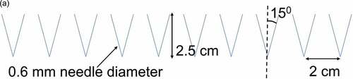
Figure 1. (Continued).

With the above considerations, first, a two-dimensional structure for the 2.5-cm-thick surface hoar layer (with a 0.3-mm ice column radius) was generated (Figure 1a). This simplified structure was considered a reference structure and its effective compressive strength was determined through numerical tests. This compressive strength was considered as a reference, and weak layers of different thickness were numerically tested by varying column diameters until this reference compression strength was achieved. The variation in column diameter with weak layer thickness obtained in this process is discussed in results and discussion section.

Material model

The mechanical behavior of ice columns is represented by the elastoplastic material model with isotropic hardening. The von Mises stress was used for yield point assessment with the following equation:

(1) $f=\sigma -\left({\sigma }_y+H{\epsilon }^{pl}\right)=0\hspace{0.17em},$(1)

where $\sigma$, ${\sigma }_y$, H, and ${\epsilon }^{pl}$ are the von Mises stress, initial yield stress, hardening modulus, and equivalent plastic strain, respectively. Plasticity is used to define equivalent plastic strain–based damage initiation and fracture energy–based damage evolution (softening). To model near-brittle failure of ice (observed at high strain rates), damage initiation is considered at a very small equivalent plastic strain. Brittle materials generally exhibit no or very small plastic strain in comparison to ductile materials, and use of the maximum principal stress theory of failure is generally recommended. However, elastic–plastic models with different yield criteria are commonly employed in modeling brittle failure of ice (Carney et al. 2006; Sain and Narasimhan 2011; Chandel, Srivastava, and Mahajan 2014). The elastic–plastic damage material model (with the von Mises yield criterion) for ice in the present work is taken from the work of Chandel, Srivastava, and Mahajan (2014). They considered this model for ice in micromechanical modeling to estimate the macroscopic properties of snow. Also, in the present work, axial stresses in ice columns are significantly high in comparison to other stresses. In such a stress state, the von Mises failure criterion becomes equivalent to the maximum principal stress criterion. Hence, consideration of the von Mises criterion with very small damage initiation strain for failure of ice columns is reasonable. The condition for the damage initiation is defined by a parameter ${\omega }_D$, which is defined by the following equation:

(2) ${\omega }_D=\int \frac{d{\epsilon }^{pl}}{{\epsilon }_0{}^{Pl}}=1,$(2)

where ${\epsilon }^{pl}$ is the equivalent plastic strain and ${{\epsilon }_0}^{Pl}$ is the equivalent plastic strain at the onset of damage. Due to damage, a decrease in the elastic modulus and strain softening of the material occurs. The stress in the damaged material was defined as $\sigma =\left(1-D\right)\bar{\sigma }$, where $\bar{\sigma }$ is the stress in an undamaged state and D represents the scalar damage variable. For D = 1, the material was considered fully damaged or failed. The total plastic energy dissipation between the damage initiation point and complete damage (D = 1) corresponds to fracture energy $G_f$ of the material (ice). During the damage evolution, the linear variation in stress was considered and the incremental plastic displacement was related to the incremental damage variable as

(3) $\dot{D}=\frac{L{\dot{\epsilon }}^{pl}}{u_f^{pl}}=\frac{{\dot{u}}^{pl}}{u_f^{pl}}\hspace{0.17em}.$(3)

Here, L is the characteristic length of the element, ${\dot{u}}^{pl}$ is an increment of equivalent plastic displacement, and $u_f^{pl}$ is the equivalent plastic displacement at failure ($u_f^{pl}=2G_f/{\sigma }_{y0}$). $G_f$ is the fracture energy of ice and ${\sigma }_{y0}$ is the yield stress at the point of damage initiation.

A significant variation in the values of the ice properties like elastic modulus, yield stress, fracture energy, etc., has been reported in the literature on the mechanical behavior of ice. Chandel, Srivastava, and Mahajan (2014) analyzed these data (Kermani, Farzaneh, and Gagnon 2008; Schulson and Duval 2009 etc.) and used a set of ice properties to model the ice matrix in their micromechanical model to obtain the macroscopic mechanical behavior of the snow. Due to the similarity of the application, these ice properties are also used in the present model (Table 1). The ice elastic modulus and yield stress (approximate ice strength) were selected on the basis of experimental results of Kermani, Farzaneh, and Gagnon (2008) for atmospheric ice for a strain rate of 5e-5 s⁻¹ or higher. The stress–displacement curve with these ice properties is shown in Figure 1b. Because a very small damage initiation strain was considered to model a near-brittle behavior, plastic strain during hardening was very small and not visible in the stress–strain curve. Plastic strain during the linear softening is dependent on fracture energy of the material and is about 1 to 2 percent of the failure strain.

Table 1. Mechanical properties of ice used in the weak layer model.

Ice density = 917 kg/m^3, Elastic modulus = 950 MPa

Yield stress (σy) = 2.25 MPa, plasticity hardening modulus = 95 MPa

Plastic strain at which damage initiates (ε0^pl) =3 × 10^−6, fracture energy of ice (Gf) = 1.05 J/m^2

Effective mechanical behavior

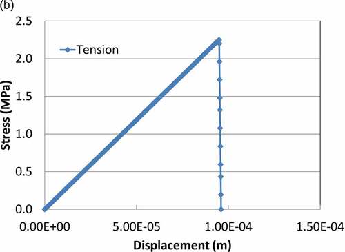
For comparison of our results with existing studies in the literature (where the weak layer is considered as a continuum or a different structural configuration), the effective mechanical properties of the weak layer model with columns were determined using a numerical FEM as shown in Figure 2. The model can be thought of as a representative volume to determine the homogenized properties of a continuum weak layer with the same width as the top slab. The inclined ice columns were discretized using two-dimensional beam elements and translational and rotational degrees of freedom of the bottom nodes in the model were constrained ($U_x=U_y={\theta }_z=0$). For uniform load distribution, all degrees of freedom (DOF) of the upper nodes of ice columns were tied to the DOF of the rigid beam, including rotation, and the load was applied through a reference node assigned to this beam. Relative rotation between the rigid beam and ice columns at the tied nodes was also constrained. The rigid slab was considered to determine the true mechanical behavior of the weak layer. A deformable slab (compliant slab) was not considered because its own deformation is expected to influence the weak layer’s mechanical behavior. While applying the vertical load at the reference node of the rigid beam, horizontal displacement was not constrained. No influence of this consideration on the results was noted because horizontal displacement ($U_x$) during application of the vertical load was negligible in comparison to vertical displacement ($U_y$).

Figure 2. Finite element model with boundary conditions for estimating the effective mechanical behavior of the surface hoar layer when replaced by a continuum weak layer. DOF = degrees of freedom.

To determine the Young’s modulus and shear modulus, the model was loaded in normal and shear modes, respectively. To determine the fracture energy and failure properties, the model was applied with normal, shear, and combined loads. For combined loading, both shear and normal loads were applied simultaneously and increased linearly until failure of the weak layer. The combined loading also helped in generating the fracture energy versus slope curve. At failure, the reaction force components at the bottom nodes were used to obtain the failure stresses. The effective stress was calculated by dividing the force by an effective area (Length × Width of the continuum weak layer), and strain was calculated by dividing the displacement components of the rigid beam reference node by the weak layer thickness. The Young’s modulus and shear modulus were estimated from the slope of the effective stress–strain curve of the weak layer in the elastic region. Peak normal and shear stresses in the stress–strain curve were used to obtain the failure curve. Total energy dissipation (Damage energy (DMD) + Plastic dissipation energy (PD) after peak stress) at failure (when the reaction force in the bottom nodes becomes zero) was divided by the effective weak layer cross-sectional area to obtain the fracture energy.

PST simulation

For numerical PSTs, an isolated column of snow was idealized as a three-layer snow cover consisting of a weak surface hoar layer sandwiched between two homogeneous snow layers (Figure 3a). Keeping in mind the short timescale of the PST (a few seconds), the mechanical behavior of the top and bottom snow slabs was considered isotropic and linear elastic. Due to the periodicity assumption of the columns in the weak layer in the out-of-plane direction, the three-dimensional PST problem was simplified to two dimensions with the top and bottom slabs being represented by plane stress elements. Here the plane stress assumption is more suitable because the columns are assumed to be repeated in the slab width direction in such a way that each set supports only a thin section (5 mm width) of the slab. The inclined ice columns of the weak layer were discretized using two-dimensional beam elements. A beam element used for ice columns has three DOF, two translations, and one rotation. The plane stress element used for slab has two translational DOF. Therefore, to connect these two different types of elements, the column end nodes are attached to the top and bottom slabs and their translation depends on motion/deformation of the top and bottom slab nodes to which they are attached. However, rotation of the end (near the slab–weak layer interface) elements of the columns with respect to the slabs is constrained. Intermediate column nodes can move as per deformation in the ice columns during interaction with the saw. To focus on fracture propagation in the weak snow layer, failure of homogeneous snow layers (top and bottom slabs) was not considered. This assumption is expected to influence the values of CCL and FPS, especially for the low-density top slab, which was likely to fail before CCL or during the early phase of fracture propagation.

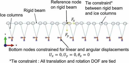
Figure 3. (a) Boundary conditions for numerical propagation saw test (PST) and (b) identification of crack tip.

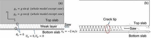
To reduce the computational time, a saw with a speed of 2 m/s (similar to Gaume, van Herwijnen et al. 2015) was used to cut the weak layer. This saw speed is much higher than the normal cutting speed in PSTs (~0.1 m/s) but much lower than the FPS during dynamic fracture propagation and is not expected to affect the results significantly. To assess the effect of saw speed on the results, for a particular PST setup, simulations were carried out for different saw speeds (0.2, 0.4, 1, 2 m/s). The boundary conditions applied in the numerical PST are shown in Figure 3a. The bottom nodes of the bottom slab were fully constrained; the interface nodes of the top and bottom slabs with weak layer were constrained for rotation. ABAQUS (2012) was used for the numerical solution. To avoid the penetration of the saw into the beam elements, a surface-to-surface contact algorithm was used between the saw and beam elements.

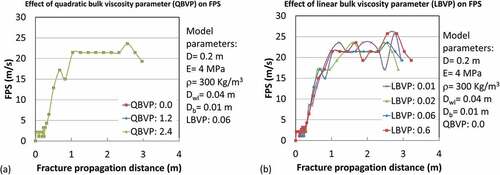
The PST simulation was carried out in two steps. In the first step, static analysis was carried out to obtain the stress distribution in the snow layers under the gravity load. In the second step, the results of the first step were imported as an initial condition, the saw was assigned velocity to cut the weak layer, and dynamic analysis was carried out. In these analyses, the discretized differential equations of static and dynamic equilibrium were solved (Bathe 2003). To damp ringing during dynamic simulations, as suggested in ABAQUS, linear and quadratic bulk viscosity parameters were used. The influence of bulk viscosity parameters on PST simulation results was investigated by varying them and found to be negligible. Details of model dimensions, layer properties, and other parameters used in these PST simulations are provided in Table 2. In a PST simulation, a point on the slab–weak layer interface was identified as a crack tip if the column at this point was intact and of all the columns to its right had failed (Figure 3b). The CCL and FPS were estimated by tracking the location of the crack tip at uniform time intervals of 0.01 seconds. The average value of FPS for a PST was obtained by averaging FPS values along the slab length after CCL was reached.

Table 2. Details of parameters used for numerical propagation saw test (PST) simulations.

1. PST model dimensions
Snow layers: Length, 3.5 m; width, 0.005 m. Cutting saw: Length, 0.04 m; width, 0.005 m
2. Snow layers and cutting saw properties
Snow layer	Thickness (m)	Element type	Mechanical model	Density (kg/m^3)	E (MPa)	v
Top slab	0.2–1.0	Plane stress	Elastic	100–500	0.1–50	0.2
Bottom slab	0.01–1.0	Plane stress	Elastic	300	4	0.2
Weak layer	0.005–0.04	Two-dimensional beam	Elastoplastic damage	Given in Table 1
Cutting saw	0.004	Plane stress	Elastic	7,800	1.0E+05	0.3

Results and discussion

Effective mechanical behavior of the weak layer

For comparison of our results with weak layer properties and models previously reported in the literature, the effective mechanical behavior of surface hoar layers for different thicknesses was characterized in terms of stress–strain curves, elastic modulus, failure curves, and fracture energy. Before presenting the results on the effective mechanical behavior of the weak layer, the variation in weak layer column diameter with thickness is shown. This variation resulted while meeting the assumption of no variation in compression strength of weak layer with thickness. The radius of inclined columns of the weak layer was nearly same for 0.5- and 1-cm-thick weak layers, whereas it increased approximately linearly for thicker weak layers (Figure 4a).

Figure 4. Effective mechanical behavior of the weak layer. (a) Variation in ice column radius with the weak layer thickness, (b) stress–strain curves for the 4-cm-thick weak layer, (c) variation in the elastic and shear moduli with weak layer thickness, (d) failure curves of weak layers of different thicknesses (negative normal stress represent compression), (e) variation in the weak layer fracture energy with weak layer thickness (tension, compression, and shear modes), and (f) variation in the weak layer fracture energy with loading angle with respect to slope normal (for the 4-cm-thick weak layer).

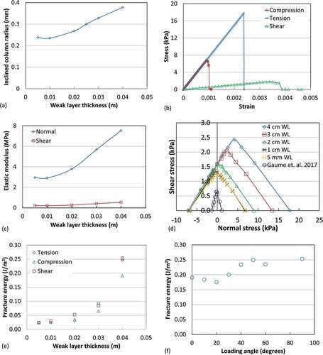
The elastic moduli of the weak layer were determined from the initial slope of the stress–strain curves (Figure 4b) and were nearly the same in tension and compression modes. The variation in the normal and shear elastic modulus with the weak layer thickness is shown in Figure 4c. The elastic modulus was significantly higher in comparison to the shear modulus. Both increased with the weak layer thickness, but the influence of the weak layer thickness on the normal modulus was significantly higher and was due to the variation in ice column diameter with weak layer thickness. Though the increase in elastic modulus with thickness here may seem contrary to intuition, it is important to understand that snow is a highly porous material with large variation and scatter in its properties due to variation in its microstructure, even for the same density; that is, a snow sample of the same density and thickness may have different properties. Hence, an increase in the weak layer model elastic modulus with thickness is not unlikely. The values of the elastic modulus were close to the values for low-density snow reported in the literature (Shapiro et al. 1997; Scapozza 2004; Köchle and Schneebeli 2014; van Herwijnen et al. 2016; Reuter, Calonne, and Adams 2019). The ratio of shear and normal elastic modulus (0.07–0.078) was significantly low in comparison to the commonly observed ratio in homogeneous materials, which was due to the anisotropic weak layer geometry and because we did not consider the infills within the weak layer. The presence of infills, like new snow, may increase the shear modulus of the weak layer because infills may also contribute toward resistance to shear deformation.

Failure curves of weak layers of different thicknesses are shown in Figure 4d. The assumption of ice column diameter variation with thickness resulted in nearly the same compression and shear strength for different weak layer thicknesses, although with large variation in tension strength. The weak layer normal strength in compression and tension modes was significantly higher and the shear strength was about two times compared to the values used by Gaume, van Herwijnen et al. (2015; DEM). The failure curve of Gaume, van Herwijnen et al. (2015) corresponds to preselected macroscopic weak layer properties, whereas our weak layer macroscopic properties were obtained from microscopic properties (ice properties and geometrical configuration of ice columns) of the weak layer. The shape and strength values in failure envelopes were close to those reported by Bobillier et al. (2020) in their micromechanical DEM. The shear strength values were close to the values reported by others (Fohn, Camponovo, and Krusi 1998; Jamieson and Schweizer 2000; Schweizer, Jamieson, and Schneebeli 2003; Reiweger and Schweizer 2010, 2013; Reuter, Calonne, and Adams 2019) for weak snow layers.

The failure envelope here represents the homogenized properties of a truss-like ice structure whose properties depend on ice properties, microstructure, and dimensions of the ice columns. This is unlike homogeneous materials in which the failure envelope does not expand with thickness. The variations observed in the failure curves (expansion of the failure envelope in tension but constant compressive strength) were due to the increase in ice column diameter with thickness. The observed expansion in the failure envelope was also due to the difference in the ice column failure process in compression and tension. In compression mode, axial compressive load enhances the flexural stresses in the column due to slab bending (buckling, eccentricity of the axial load), leading to failure of the weak layer at a lower macroscopic load. In tension mode, axial (tensile) load works against the buckling processes, leading to weak layer failure at a higher macroscopic load. An increase in column diameter reduces the buckling effect under compression and helps to attain the constant compressive strength for different thicknesses. But this increase in column diameter tends to increase the weak layer strength in tension (expansion of the failure envelope). Therefore, expansion of the failure envelope can be attributed to the microscopic failure processes in the ice column. Even if the column diameter is kept constant, expansion of the failure envelope will not be eliminated; instead, it will be dominant in the compression–shear stress quadrant rather than the tension–shear stress quadrant of the failure curve. In a PST simulation, the weak layer generally experiences compressive–shear load rather than tensile load. Hence, although the failure envelope expands in tension, it is not expected to influence the PST simulation results.

The obtained values of fracture energy (0.025–0.25 J/m²; Figure 4e) were in good agreement with those obtained in field PSTs for CCL (Sigrist 2006; Sigrist and Schweizer 2007: 0.04–0.09 J/m²; van Herwijnen et al. 2016: 0.08–2.7 J/m²; Schweizer et al. 2016: 0.5–2.2 J/m²) and using field measurements of slab avalanches and theoretical expressions for fracture toughness (McClung 2005, 2007: 0.001–0.2 J/m²). Most of these values in the literature are for mode II or mixed mode fracture of the weak layer. In our weak layer model, fracture energies in normal and shear modes increased with the increase in weak layer thickness, as seen in Figure 4e. The fracture energy in both normal (mode I, tension and compression) and shear (mode II) modes was nearly same for thin weak layers, whereas in thicker weak layers the fracture energy in compression mode was slightly lower in comparison to tension and shear modes. This was because in compression mode the inclined columns experienced both axial and lateral loads and consideration of large deformation resulted in enhanced stresses in the columns. For a 4-cm weak layer (Figure 4f) the fracture energy increased when the mode of loading changed from normal (compression, 0° loading angle) to mixed mode. This variation was due to the change in loading conditions with respect to the weak layer structure on varying the slope angle. The values of weak layer fracture energy in the present model were well within the range reported in the literature and were nearly of the same order for mode I (compression) and mode II. The variation in fracture energy of a weak layer with a change in mode of loading has not been reported in the literature. This may be due to variability in snow properties and limitations in field PSTs to obtain same weak layer microstructure with variation in slope angle. van Herwijnen et al. (2016) used experimental PST data of Gauthier and Jamieson (2008) in which they reported PST experiments over 0° slope, but mode I fracture energy estimates from these data have not been reported explicitly.

For homogenous snow, Kirchner, Michot, and Schweizer (2002) suggested nearly equal fracture toughness in tension and shear modes, whereas Schweizer, Michot, and Kirchner (2004) suggested a ratio of 1.4 between fracture toughness in tension and shear modes. Rosendahl and Weißgraeber (2020), on the basis of experiments by Heierli, Gumbsch, and Sherman (2012) on porous glass, suggested that the fracture energy in mode I (compression) was about two orders higher in comparison to mode II. A detailed experimental study is needed to establish the ratio of mode I (compression) and mode II fracture energies of weak snow layers.

It is also important to highlight that the proposed ice column model for the weak layer is a simplified model and has its own limitations. The weak layer model proposed here represents only limited scenarios (out of many other possible ones) of variation in snow properties with thickness. The weak layers with different thicknesses are actually different materials (contrary to homogeneous materials in which properties do not change with thickness) with different microstructures, properties, and failure criteria. Hence, a significant variation in snow properties with thickness is not unlikely. However, the closeness of effective mechanical properties with low-density snow suggests a close resemblance to a typical weak snow layer.

CCL and FPS in PST simulations

In this section, results of a parametric study on the influence of snow cover properties and slope angle on the CCL and FPS are presented. Results from previous studies (Heierli 2005; Heierli, Gumbsch, and Zaiser 2008; Gaume, van Herwijnen et al. 2015; Gaume et al. 2017) are also shown for comparison. While calculating the CCL using the weak layer collapse (WLC) model, the effective weak layer fracture energy values obtained in the present work (which varies from 0.024 to 0.2 J/m² for weak layer thicknesses of 5 mm to 4 cm) are used. A typical failure of the model weak layer is shown in Figure 3b. It is important to highlight that before carrying out this study, the effect of saw speed and bulk viscosity parameters (used to damp ringing) on simulation results were studied and no major influence was noted (see Figures A2 and A3 in Appendix 1).

Critical crack length

The influence of snow cover properties and the slope angle on the CCL is shown in Figure 5. The obtained CCL values (0.1–0.6 m) are close to the experimental values reported in the literature (Sigrist and Schweizer 2007; Gauthier and Jamieson 2008; Schweizer, van Herwijnen, and Reuter 2011; Bair et. al. 2012; Schweizer et al. 2016). The CCL decreased with top slab density and thickness, whereas a reverse variation was observed for top slab elastic modulus, weak layer thickness, and slope angle. The bottom slab thickness did not affect the CCL. The influence of the top slab density, considering the density-dependent elastic modulus (Scapozza 2004), is shown in Figure 5a. For low densities (below 300 kg/m³), the CCL decreased with density, and a reverse trend was observed for higher densities. These results indicate the dominance of top slab elastic modulus over density for densities greater than 300 kg/m³.

Figure 5. Variation in CCL with (a) top slab density ρ, (b) top slab thickness D, (c) top slab elastic modulus E, (d) bottom slab thickness D_b, (e) weak layer thickness D_wl, (f) slope angle ψ. W_f = weak layer fracture energy; AM = analytical model; DEM = discrete element model; FEM = finite element model; CCL = critical crack length.

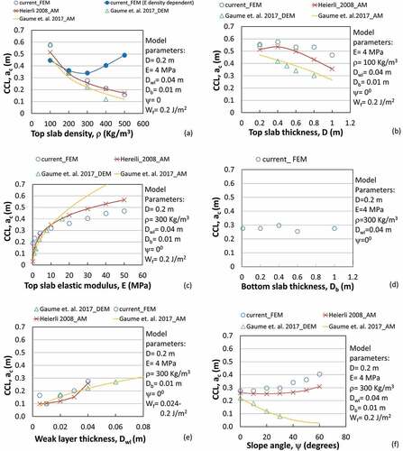
The increase in CCL with slope angle was due to a decrease in the potential energy release rate (see Figure A1 in Appendix 1) and an increase in fracture energy (Figure 4f) with slope angle. The variation in the CCL with slope angle was similar to that of the WLC model (Heierli, Gumbsch, and Zaiser 2008) but deviated from the results reported for the DEM and the analytical model (Gaume et al. 2017). However, trends of variation in CCL with the other parameters were generally similar to these two models.

An increase or no change in CCL with slope angle has also been reported in previous experimental field studies (Gauthier and Jamieson 2008; McClung 2009; Bair et al. 2012) but has not yet been established due to some inherent limitations in the experiments conducted (Gaume et al. 2017). An increase in CCL with slope angle obtained by the WLC model was due to the decrease in potential energy release rate with slope angle and constant weak layer fracture energy. The decrease in CCL with slope angle in the DEM may be due to decrease in weak layer fracture energy with slope angle.

The simulations were also carried out by introducing friction between the top and bottom slabs, but no influence on CCL was observed because CCL was reached before contact between the top and bottom slabs occurred. CCL values obtained in PSTs are generally an indicator of stability of the snow cover but do not reflect true value of CCL in natural snow cover, which is generally higher than the CCL value in PSTs.

Fracture propagation speed

The variation in the FPS with the fracture propagation distance for different top slab densities is shown in Figure 6a. Immediately after attaining the CCL, a rapid increase in the FPS was observed. Thereafter the rate of increase decreased and FPS tended toward a nearly constant value. This trend was observed in all PST simulations and was also reported by Bobillier et al. (2021). The influence of the snow cover properties and the slope angle on the average FPS is shown in Figure 7. The variation in elastic wave speed, c_e ($\approx \sqrt{E/\rho }$), is also plotted for reference. The values of FPS obtained in PST simulations were close to the experimental values (Figure 7a) reported in the literature (Johnson, Jamieson, and Stewart 2004; McClung 2005; van Herwijnen and Jamieson 2005; Gaume, van Herwijnen et al. 2015).

Figure 6. Variation in FPS with fracture propagation distance. (a) Effect of top snow slab density (kg/m³) and (b) effect of friction between top and bottom slabs. FPS = fracture propagation speed; mu: friction coefficient.

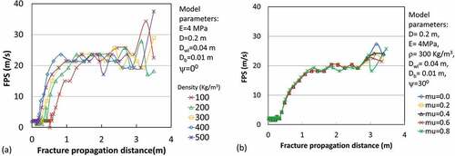
Figure 7. Variation in average FPS with (a) top slab density (experimental data) ρ, (b) top slab density (model results) ρ, (c) top slab thickness D, (d) top slab elastic modulus E, (e) weak layer thickness D_wl, (f) slope angle ψ. ce = elastic wave speed, $(\approx \sqrt{E/\rho }$), shown with dashed line in each figure. DEM = discrete element model; FEM = finite element model; PST = propagation saw test; SWM = solitary wave model; ECT = extended column test; FPS = fracture propagation speed; Exp = experimental.

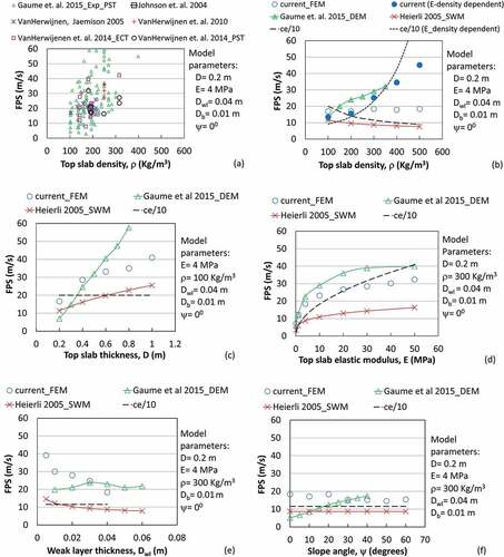
The density of the top slab did not affect the FPS unless the density-dependent elastic modulus for the top slab was considered. This is because the speed of the elastic wave slightly decreases with density if the elastic modulus is not considered a function of density and no major variation in FPS with slab density is observed. However, if the elastic modulus was considered density dependent (as per Scapozza 2004), a significant increase in elastic wave speed as well as in FPS with slab density was noted (Figure 7b). The DEM showed a strong increasing trend for FPS with the top slab density even if the elastic modulus was constant. The solitary wave model (SWM) showed a decreasing trend with the top slab density, which is due to the consideration of an inverse relation of the density with the elastic wave speed. FPS as per the SWM is given by the equation $c=\sqrt{c_0{c}_s}$, where $c_s$ is the wave velocity of a shear elastic wave given by $c_s=\sqrt{E/2\left(1+\nu \right)\rho }$ and $c_0$ is a coefficient with velocity given by $c_0=\sqrt{g{H}^2/12\left|h\right|\left(1-\nu \right)}$, where H is the slab thickness, h is the weak layer collapse height, E is the elastic modulus of the slab, g is gravitational acceleration, and $\nu$ is Poisson’s ratio.

The FPS increased with top slab elastic modulus and thickness, whereas it decreased with the thickness of the weak layer. With increasing slab thickness, the elastic wave velocity was constant but the significant increase in FPS (Figure 7c) suggests a significant contribution of slab thickness in the FPS. The increase in FPS with top slab elastic modulus (with constant density) was due to the increase in elastic wave speed. The variation in FPS with the top slab elastic modulus and thickness was in agreement with other models.

The decrease in FPS with the increase in the weak layer thickness was due to an increase in the fracture energy of the weak layer (Figure 4e). No major influence of weak layer thickness on FPS was reported in the DEM of Gaume, van Herwijnen et al. (2015). This may be because there was no major variation in weak layer fracture energy with thickness in their model. The decrease in FPS with the weak layer thickness in the SWM was due to the inverse relation of the weak layer thickness parameter (weak layer collapse height) to the FPS in their analytical model.

The FPS remained nearly constant up to 20° slope angle, with slightly lower values at higher slope angles (30° and above). This was because of a decrease in the potential energy release rate (PERR; see Figure A1 in Appendix 1) and an increase in fracture energy with slope angle. DEM results (Gaume, van Herwijnen et al. 2015) showed an increase in FPS with slope angle. This may be due to the decrease in fracture energy of their weak layer with slope angle. The analytical SWM did not consider the effect of slope angle.

There was no major influence of friction between the top and bottom slabs on FPS, as seen in Figure 6b, because of the insufficient length of fracture propagation after contact between the top and bottom slabs. A model with longer slab lengths will help in understanding the influence of friction on FPS in a better way.

Energy variations during the fracture propagation process

The energy variations in PST simulations were investigated to understand the mechanism of fracture propagation in the weak layer. The energy balance equation for PST can be written as

$W=U_e+K+\mathrm{\Gamma }$

where,

Total external work $W=W_{grav}+W_{saw}$

and W_grav is the gravitational work, W_saw is the work done by the saw, U_e is the elastic strain energy of the whole model, Γ is the energy dissipation in crack propagation (Damage energy + Plastic dissipation energy during damage evolution), and K is the kinetic energy of the whole model.

Potential energy (PE) of the system can be written as $PE=-\left(U_e-W\right)$ and PERR can be written as $\mathrm{\partial }\left(PE\right)/\mathrm{\partial }a=-\mathrm{\partial }\left(U_e-W\right)/\mathrm{\partial }a$.

In rate form (with respect to crack size), the energy balance equation can be written as

$-\frac{\mathrm{\partial }}{\mathrm{\partial }a}\left(U_e-W\right)=\frac{\mathrm{\partial }K}{\mathrm{\partial }a}+\frac{\mathrm{\partial }\mathrm{\Gamma }}{\mathrm{\partial }a}.$

For negligible kinetic energy, this equation is similar to the general energy balance equation suggested by Vachon and Hieronymus (2019) for fractures involving dissipative loss due to inelastic deformations. Energy variations in PST are combined effects of gravitational and saw work, but during fracture propagation the contribution of the saw is negligible; hence, an analysis of variation in gravitational work (due to the top slab) and associated variations in different energies during PST is presented. Released potential energy was obtained by deducting strain energy of the model from gravitational work and also used to calculate PERR. All energies were obtained as standard outputs in ABAQUS.

The variation in W_grav (top slab), U_e (whole model (WM)), released potential energy (U_e-W_grav), K (top slab), and dissipation energy, damage energy (DMD) + plastic dissipation energy (PD) of the weak layer with the fracture propagation distance is shown in Figure 8a. The damage energy here corresponds to energy dissipation due to degradation of the elastic modulus of ice resulting from failure of the weak layer. The variation in corresponding specific energies/work with fracture propagation distance is shown in Figure 8b. Figure 8b also shows the maximum stress variation in the inclined columns ahead of the failed columns (i.e., at the crack tip) with the fracture propagation distance. The CCL is also marked in these plots.

Figure 8. (a) Variation in gravitational work W (top slab), strain energy U_e (whole model), released potential energy (U_e − W) (whole model), kinetic energy K (top slab), and dissipation energy DMD + PD (weak layer) with fracture propagation distance along with CCL (0.2756 m). (b) Variation in specific energies (gravitational work, dW/da [top slab]; PERR, d(U_e − W)/da [shown positive for comparison]; strain energy, dU_e/da [whole model]; kinetic energy, dK/da (top slab), dissipation energy, d(DMD + PD)/da [weak layer]) and maximum crack tip stress with the fracture propagation distance along with CCL. CCL = critical crack length; TS: top slab; WM: whole model; WL: weak layer; PERR: potential energy release rate; DMD: damage dissipation energy; PD: plastic dissipation energy.

Prior to critical crack length

With an increase in crack size, the gravitational work on the top slab as well as strain energy of the system increased but the kinetic energy (KE) of the top slab was negligible. Energy dissipation in the weak layer is not shown prior to CCL because this energy was supplied by the saw as well as gravitational work (top slab). The specific gravitational work (top slab) as well as specific strain energy increased with crack size, although fluctuations were observed. Simulations output recorded at fixed time intervals (0.01 seconds) may correspond to variable nonequilibrium states leading to fluctuations in specific energies. The stresses in the columns ahead of the failed columns (i.e., at the crack tip) also increased with an increase in crack size.

The above energy variations were also analyzed to understand the condition for fracture propagation at the obtained CCL. The increase in crack size resulted in external work by gravitational force leading to top slab bending. This external gravitational work (prior to CCL) resulted in an increase in strain energy of the system and an increase in stresses in the weak layer ahead of the failed columns (i.e., at the crack tip). Up to 0.22 m crack length, PERR was less than the fracture energy of the weak layer (0.2 J/m²), but beyond 0.22 m crack length, PERR exceeded the fracture energy of the weak layer (fulfills the energy criterion of fracture mechanics) but crack did not propagate because stress in the column (at the crack tip) was well below the ice strength (~2.25 MPa). This may be due to dissipation of increased energy release into failure of a column ahead of the intact column at the crack tip as observed in the simulation. At CCL (0.2756 m), stress in the column (at the crack tip) also exceeded the ice strength, leading to crack propagation in the weak layer. This outcome suggests that if such energy dissipation processes (not contributing to the crack extension) are expected prior to CCL, use of only the energy criterion may underestimate CCL. In such a scenario, in addition to the energy criterion, consideration of fulfillment of material failure criterion near the crack tip (columns here) may provide better estimates of CCL. Such coupled criteria have been used in other materials for cracking of damaged materials (Li et al. 2019).

After onset of dynamic fracture propagation

Once CCL was reached, both gravitational work and strain energy (whole model) continued to increase. In addition, the kinetic energy (top slab) and energy dissipation in the weak layer alsoincreased (Figure 8a). After CCL was reached, the source of energy dissipation in the weak layer was the difference between gravitational work and the sum of strain energy (whole model) and KE (top slab). These specific energies are plotted in Figure 8b. Immediately after CCL, due to the sudden increase in FPS, the top slab does not come down fast enough, resulting in a decrease in specific gravitational work and specific strain energy of the system (between 0.2756 and 0.34 m) and retaining some energy in the form of gravitational potential energy. This gravitational potential energy entered the system between 0.34 and 0.6 m, leading to an increase in specific gravitational work and PERR. Thereafter, the PERR and specific kinetic energy of the top slab kept increasing but the specific dissipation energy (weak layer) and specific strain energy (whole model) tended toward nearly constant values. This variation in specific energies suggests that beyond the CCL the released potential energy is used mainly (1) for failure of weak layer during fracture propagation (nearly constant specific dissipation energy) (2) to increase the KE of the top slab. The criterion of distribution of the gravitational work for these two purposes was studied on the basis of FPS and the variation in KE.

The initial increase in FPS (with fracture propagation distance) at a nearly constant rate suggests a continuous increase in available energy for the fracture propagation (Figure 9a). But the rate of increase of the FPS decreased as the KE of the top slab exceeded the energy used for fracture propagation in the weak layer. This resulted in a nearly constant FPS plateau after the crack reached 0.4 m. These results suggest that below a particular crack size, when the KE of the top slab is not significant, most of the released energy is utilized for fracture propagation (failure of the weak layer), but when the KE of the top slab becomes significant, energy available for fracture propagation is restricted. A higher top slab elastic modulus resulted in higher elastic wave speed ($c\approx \sqrt{E/\rho })$ and faster transfer of the released energy to the top slab and weak layer over a longer distance. This resulted in less energy availability to increase the KE of the top slab (Figure 9c) and higher limiting FPS at a higher propagation distance (Figure 9b).

Figure 9. (a) Variation in kinetic energy (top slab), dissipation energy (weak layer), and FPS with fracture propagation distance, (b) influence of the top slab elastic modulus on FPS, (c) influence of the top slab elastic modulus on the kinetic energy of the top slab, and (d) influence of the top slab density on the kinetic energy of the top slab. TS = top slab; WL = weak layer; FPS = fracture propagation speed.

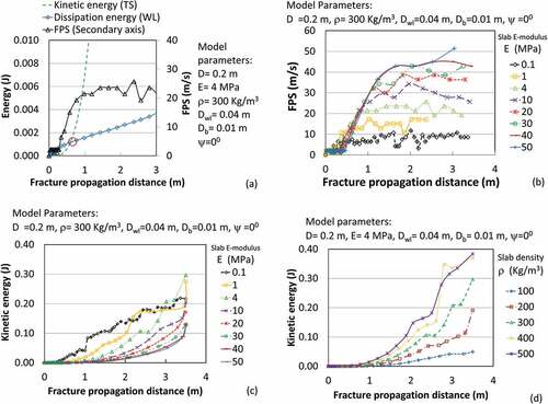
But with an increase in the top slab density (with constant elastic modulus) the kinetic energy of the top slab increased (Figure 9d) while FPS remained unaffected (Figure 7a). The higher top slab density resulted in higher gravitational work but reduced energy availability for fracture propagation due to the decrease in elastic wave speed ($c\approx \sqrt{E/\rho })$ and higher top slab KE. As a result, top slab density had no major influence on FPS. The observations regarding the decrease in FPS with the increase in weak layer thickness (and increase in fracture energy, Figure 7e) suggest an inverse relation of FPS with the weak layer fracture energy. This is because, the energy available for weak layer failure during a time step may fail a low fracture energy weak layer over a longer distance in comparison to higher fracture energy weak layer, resulting in higher FPS.

The above observations suggest that the distribution of the gravitational work during fracture propagation is governed by the elastic modulus and kinetic energy of the top slab. FPS during dynamic fracture propagation is also influenced by the weak layer fracture energy. These results on the influence of elastic modulus and weak layer fracture energy on FPS are also supported by the dynamic theory of fracture mechanics (Bouchbinder, Fineberg, and Marder 2010).

Conclusions

A model for a surface hoar–like weak snow layer was proposed and used to investigate the fracture propagation process in weak snow layers. The weak layer was modeled as a periodic structure of inclined ice columns and the effective mechanical properties of this model layer were reasonably close to the properties of the low-density natural snow reported in the literature.

This weak layer model was used in numerical propagation saw tests and the influence of top slab, weak layer, and slope angle on CCL and FPS were studied through a parametric study. With the proposed weak layer model, the obtained CCL and FPS values are in good agreement with the values reported in the literature. Variation in CCL with top slab properties and weak layer thickness is in good agreement with the previously proposed models with few exceptions. CCL variation with slope angle is in good agreement with the energy-based model of Heierli, Gumbsch, and Zaiser (2008) but disagrees with the DEM results of Gaume et al. (2017). Variation in FPS with top slab thickness and elastic modulus is in line with other models, but significant deviations are observed with respect to the influence of the top slab density, weak layer thickness, and slope angle. Differences in our results with respect to the results of the DEM are probably due to the difference in variation in weak layer fracture energy with thickness and slope angle. The reason for the difference in the results for the influence of top slab density on FPS is yet to be understood. Because failure of the top slab was not considered in present work, the obtained values of CCL and FPS may be overestimated for low-density top slabs, which are likely to fail before CCL or during the early phase of fracture propagation.

Through energy analysis in PST simulations, it is shown that CCL in PST is determined by a coupled energy- and stress-based criterion and the dynamic fracture propagation process in the weak layer is governed by the top slab elastic modulus, weak layer fracture energy, and inertia of the overlying slab. The influence of the top slab elastic modulus and weak layer fracture energy on FPS also confirms the compliance with the theory of dynamic fracture mechanics.

Overall, the proposed weak layer model simulates the fracture propagation process in numerical PSTs reasonably well, but deviations with respect to previous models emphasize the need for detailed experimental investigations. Experiments are needed to validate the influence of slope angle on CCL and the influence of top slab density and weak layer fracture energy on FPS.

Though the proposed weak layer model performed reasonably well and provided reasonably good insight into the fracture propagation process, further improvements in the weak layer geometry are required for a more realistic weak layer structure. In addition, further work is needed to understand the role of infills (like new snow) and contact and friction between the top and bottom slabs and failure of the top slab on the fracture propagation process.

Authors’ contributions

All authors contributed to the conceptulization of the models used in the study. Modeling, simulation, data processing, and preliminary analysis were carried out by AU. The first draft of the article was written by AU and all authors commented on preliminary analysis and previous versions of the article. PM supervised the entire work. All authors read and approved the final article.

Acknowledgments

The authors acknowledge the support provided by the director of DGRE. The authors are also grateful to the reviewers for their valuable comments that helped improve this article.

Disclosure statement

No potential conflict of interest was reported by the authors.

Additional information

Funding

This work was supported by the Defence Geoinformatics Research Establishment, DRDO.

Appendix 1

Variation of potential energy release rate with slope angle

To obtain PERR, the strain energy of the PST system (U_e) was obtained through static finite element simulation for two different crack sizes (0.2 and 0.22 m) and the potential energy release rate (dU_e/da) was calculated. PERR was estimated for different slope angles and the obtained variation in PERR with slope angle is shown in Figure A1.

Figure A1. Variation in potential energy release rate with slope angle. D = top slab thickness; E = top slab elastic modulus; ρ = top slab density; D_wl = weak layer thickness; D_b = bottom slab thickness; a = crack size.

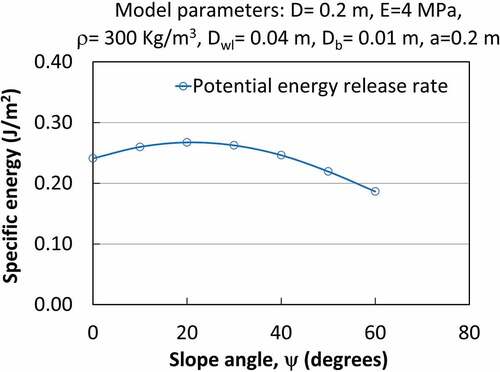
Figure A2. Effect of saw speed on PST simulation results. CCL: Critical crack length; FPS: Fracture propagation speed; PST: Propagation saw test.

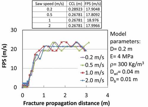
Figure A3. Effect of (a) quadratic (b) linear bulk viscosity parameter on PST simulation results. FPS: Fracture propagation speed; PST: Propagation saw test.

References

- ABAQUS. 2012. Analysis user's manual (version 6.12). Dassault Systemes Simulia, Inc.
- Bader, H. P., and B. Slam. 1990. On the mechanics of snow slab release. Cold Region Science and Technology 17 (3):288–300. doi:10.1016/S0165-232X(05)80007-2.
- Bair, E., R. Simenhois, K. Birkeland, and J. Dozier. 2012. A field study on failure of storm snow slab avalanches. Cold Region Science and Technology 17:20–28. doi:10.1016/j.coldregions.2012.02.007.
- Bathe, K. J. 2003. Finite element procedures. New Delhi: Prentice-Hall of India Private Limited.
- Bobillier, G., B. Bergfeld, A. Capelli, J. Dual, J. Gaume, A. van Herwijnen, and J. Schweizer. 2020. Micromechanical modeling of snow failure. The Cryosphere 14 (1):39–49. doi:10.5194/tc-14-39.
- Bobillier, G., B. Bergfeld, J. Dual, J. Gaume, A. van Herwijnen, and J. Schweizer. 2021. Micromechanical insights into the dynamics of crack propagation in snow fracture experiments. Scientific Reports 11 (1):11711. doi:10.1038/s41598-021-90910-3.
- Bouchbinder, E., J. Fineberg, and M. Marder. 2010. Dynamics of simple cracks. Annual Review of Condensed Matter Physics 1 (1):371–95. doi:10.1146/annurev-conmatphys-070909-104019.
- Carney, K. S., D. J. Benson, P. DuBois, and R. Lee. 2006. A phenomenological high strain rate model with failure for ice. International Journal of Solids and Structures 43 (25–26):7820–39. doi:10.1016/j.ijsolstr.2006.04.005.
- Chandel, C., P. K. Srivastava, and P. Mahajan. 2014. Micromechanical analysis of deformation of snow using X-ray tomography. Cold Regions Science and Technology 101:14–23. doi:10.1016/j.coldregions.2014.01.005.
- Fohn, P. M. B., C. Camponovo, and G. Krusi. 1998. Mechanical and structural properties of weak snow layers measured in-situ. Annals of Glaciology 26:1–6. doi:10.3189/1998AoG26-1-1-6.
- Gaume, J., G. Chambon, N. Eckert, and M. Naaim. 2013. Influence of weak-layer heterogeneity on snow slab avalanche release: Application to the evaluation of avalanche release depths. Journal of Glaciology 59 (215):423–37.
- Gaume, J., G. Chambon, N. Eckert, M. Naaim, and J. Schweizer. 2015. Influence of weak-layer heterogeneity and slab properties on slab tensile failure propensity and avalanche release area. The Cryosphere 9 (2):795–804. doi:10.5194/tc-9-795-2015.
- Gaume, J., A. van Herwijnen, G. Chambon, K. W. Birkeland, and J. Schweizer. 2015. Modelling of crack propagation in weak snowpack layers using the discrete element method. The Cryosphere 9 (5):1915–32. doi:10.5194/tc-9-1915-2015.
- Gaume, J., A. van Herwijnen, G. Chambon, N. Wever, and J. Schweizer. 2017. Snow fracture in relation to slab avalanche release: Critical state for the onset of crack propagation. The Cryosphere 11 (1):217–28. doi:10.5194/tc-11-217-2017.
- Gauthier, D., and B. Jamieson. 2008. Evaluation of a prototype field test for fracture and failure propagation propensity in weak snowpack layers. Cold Region Science and Technology 51 (2–3):87–97. doi:10.1016/j.coldregions.2007.04.005.
- Haefeli, R. 1963. Stress transformations, tensile strengths and rupture processes of the snow cover. In Ice and snow, ed. W. D. Kingery I’d., 560–75. Cambridge, MA: M. I. T. Press.
- Heierli, J. 2005. Solitary fracture waves in metastable snow stratifications. Journal of Geophysical Research (Earth Surface) 110 (F9):F02008. doi:10.1029/2004JF000178.
- Heierli, J., P. Gumbsch, and D. Sherman. 2012. Anticrack-type fracture in brittle foam under compressive stress. Science Scripta Materialia 67 (1):96–99. doi:10.1016/j.scriptamat.2012.03.032.
- Heierli, J., P. Gumbsch, and M. Zaiser. 2008. Anticrack nucleation as triggering mechanism for slab avalanches. Science 321 (5886):240–43. doi:10.1126/science.1153948.
- Jamieson, J. B., and J. Schweizer. 2000. Texture and strength changes of buried surface hoar layers with implications for dry snow-slab avalanche release. Journal of Glaciololgy 46 (152):151–60. doi:10.3189/172756500781833278.
- Johnson B. C. 2000. Remotely triggered slab avalanches. MSc thesis, Department of Civil Engineering, University of Calgary, Calgary, Canada.
- Johnson, B. C., J. B. Jamieson, and R. R. Stewart. 2004. Seismic measurements of fracture speed in a weak snowpack layer. Cold Region Science and Technology 40 (1–2):41–45. doi:10.1016/j.coldregions.2004.05.003.
- Kermani, M., M. Farzaneh, and R. Gagnon. 2008. Bending strength and effective modulus of atmospheric ice. Cold Region Science and Technology 53 (2):162–69. doi:10.1016/j.coldregions.2007.08.006.
- Kirchner, H. O. K., G. Michot, and J. Schweizer. 2002. Fracture toughness of snow in shear and tension. Scripta Materialia 46 (6):425–29. doi:10.1016/S1359-6462(02)00007-6.
- Köchle, B., and M. Schneebeli. 2014. Three-dimensional microstructure and numerical calculation of elastic properties of alpine snow with a focus on weak layers. Journal of Glaciology 60 (222):705–13. doi:10.3189/2014JoG13J220.
- Li, J., D. Leguillon, E. Martin, and X. Zhang. 2019. Numerical implementation of the coupled criterion for damaged materials. International Journal of Solids and Structures, Elsevier 165:93–103. doi:10.1016/j.ijsolstr.2019.01.025.
- Mahajan, P., K. Kalakunta, and C. Chandel. 2010. Numerical simulation of failure in a layered thin snowpack under skier load. Annals of Glaciology 51 (54):169–75. doi:10.3189/172756410791386436.
- Mahajan, P., and S. Senthil. 2004. Cohesive element modelling of crack growth in layered snowpack. Cold Region Science and Technology 40 (1–2):111–22. doi:10.1016/j.coldregions.2004.06.006.
- McClung, D. M. 1979. Shear fracture precipitated by strain softening as a mechanism of dry avalanche release. Journal of Geophysical Research 84 (B7):3519–26. doi:10.1029/JB084iB07p03519.
- McClung, D. M. 1980. Fracture mechanical models of dry slab avalanche release. Journal of Geophysical Research 86 (B11):10783–90. doi:10.1029/JB086iB11p10783.
- McClung, D. M. 1987. Mechanics of snow slab failure from a geotechnical perspective. Davos Symposium on Avalanche Formation, Movement and Effects (IAHS Publication) 162:475–508.
- McClung, D. M. 2005. Approximate estimates of fracture speeds for dry slab avalanches. Geophysical Research Letters 32 (8):L08406. doi:10.1029/2005GL022391.
- McClung, D. M. 2007. Fracture energy applicable to dry snow slab avalanche release. Geophysical Research Letters 34 (2):1–5. doi:10.1029/2006GL028238.
- McClung, D. M. 2009. Dry snow slab quasi-brittle fracture initiation and verification from field tests. Journal of Geophysical Research 114 (F1):F01022. doi:10.1029/2007JF000913.
- Mulak, D., and J. Gaume. 2019. Numerical investigation of the mixed-mode failure of snow. Computational Particle Mechanics 6 (3):439–47. doi:10.1007/s40571-019-00224-5.
- Perla, R. I., and E. R. LaChapelle. 1970. A theory of snow slab failure. Journal of Geophysical Research 75 (36):7619–27. doi:10.1029/JC075i036p07619.
- Reiweger, I., and J. Schweizer. 2010. Failure of a layer of buried surface hoar. Geophysical Research Letters 37 (24):L24501. doi:10.1029/2010GL045433.
- Reiweger, I., and J. Schweizer. 2013. Weak layer fracture: Facets and depth hoar. The Cryosphere 7 (5):1447–53. doi:10.5194/tc-7-1447-2013.
- Reuter, B., N. Calonne, and E. Adams. 2019. Shear failure of weak snow layers in the first hours after burial. The Cryosphere Discuss. doi:10.5194/tc-2018-268.
- Rosendahl, P. L., and P. Weißgraeber. 2020. Modeling snow slab avalanches caused by weak-layer failure-Part 2: Coupled mixed-mode criterion for skier-triggered anticracks. The Cryosphere 14 (1):131–45. doi:10.5194/tc-14-131-2020.
- Sain, T., and R. Narasimhan. 2011. Constitutive modeling of ice in the high strain rate regime. International Journal of Solids and Structures 48 (5):817–27. doi:10.1016/j.ijsolstr.2010.11.016.
- Scapozza, C. 2004. Entwicklung eines dichte- und temperaturabhängigen Stoffgesetzes zur Beschreibung des visko-elastischen Verhaltens von Schnee. PhD thesis, ETH Zürich. doi:10.3929/ethz-a-004680249.
- Schulson, E. M., and P. Duval. 2009. Creep and fracture of ice. Cambridge: Cambridge University Press.
- Schweizer, J., J. B. Jamieson, and M. Schneebeli. 2003. Snow avalanche formation. Review of Geophysics 41 (4):4/1016. doi:10.1029/2002RG000123.
- Schweizer, J., G. Michot, and H. O. K. Kirchner. 2004. On the fracture toughness of snow. Annals of Glaciology 38:1–8. doi:10.3189/172756404781814906.
- Schweizer, J., B. Reuter, A. van Herwijnen, B. Richter, and J. Gaume. 2016. Temporal evolution of crack propagation propensity in snow in relation to slab and weak layer properties. The Cryosphere 10 (6):2637–53. doi:10.5194/tc-10-2637-2016.
- Schweizer, J., A. van Herwijnen, and B. Reuter. 2011. Measurements of weak layer fracture energy. Cold Region Science and Technology 69 (2–3):139–44. doi:10.1016/j.coldregions.2011.06.004.
- Shapiro, L. H., J. B. Johnson, M. Sturm, and G. L. Blaisdell. 1997. Snow mechanics. CRREL Report 97 (3).
- Sigrist, C. 2006. Measurement of fracture mechanical properties of snow and application to dry snow slab avalanches. PhD thesis, ETH Zurich, Diss. ETH No. 16736.
- Sigrist, C., and J. Schweizer. 2007. Critical energy release rates of weak snowpack layers determined in field experiments. Geophysical Research Letters 34 (3):L03502. doi:10.1029/2006GL028576.
- Vachon, R., and C. F. Hieronymus. 2019. Mechanical energy balance and apparent fracture toughness for dykes in elastoplastic host rock with large-scale yielding. Geophysical Journal International 219 (3):1786–804. doi:10.1093/gji/ggz383.
- van Herwijnen, A., J. Gaume, E. H. Bair, B. Reuter, K. W. Birkeland, and J. Schweizer. 2016. Estimating the effective elastic modulus and specific fracture energy of snowpack layers from field experiments. Journal of Glaciology 62 (236):997–1007. doi:10.1017/jog.2016.90.
- van Herwijnen, A., and B. Jamieson. 2005. High-speed photography of fractures in weak snowpack layers. Cold Regions Science and Technology 43 (1–2):71–82. doi:10.1016/j.coldregions.2005.05.005.