Characterizing vegetation and return periods in avalanche paths using lidar and aerial imagery

ABSTRACT

Snow avalanches are a hazard and ecological disturbance across mountain landscapes worldwide. Understanding how avalanche frequency affects forests and vegetation improves infrastructure planning, risk management, and avalanche forecasting. We implemented a novel approach using lidar, aerial imagery, and a random forest model to classify imagery-observed vegetation within avalanche paths in southern Glacier National Park, Montana, USA. We calculated spatially explicit avalanche return periods using a physically based spatial interpolation method and characterized the vegetation within those return period zones. The automated vegetation classification model differed slightly between avalanche paths, but the combination of lidar and spectral signature metrics provided the best accuracy (88–92 percent) for predicting vegetation classes within complex avalanche terrain rather than lidar or spectral signature metrics alone. The highest frequency avalanche return periods were broadly characterized by grassland and shrubland, but the influence of topography greatly influences the vegetation classes as well as the return periods. Furthermore, statistically significant differences in lidar-derived vegetation canopy height exist between categorical return periods. The ability to characterize vegetation within various avalanche return periods using remote sensing data provides land use planners and avalanche forecasters a tool for assessing the spatial extent of large-magnitude avalanches in individual avalanche paths.

KEYWORDS:

• Snow avalanche
• remote sensing
• dendrochronology

Introduction

Snow avalanche (hereafter avalanche) disturbance across the landscape is a hazard and an important ecological process in mountain locations throughout the world. Avalanches have the potential to affect alpine ecosystems, forests, and riparian zones, particularly in the case of large-magnitude avalanches. Avalanches contribute to animal habitat (Waller and Mace 1997), change the species of flora along an elevational gradient, and modify forest structure (Rixen et al. 2007). Avalanches also pose a substantial hazard, and understanding the interaction of avalanche frequency and runout in forested terrain is important for human safety, transportation corridors, and infrastructure. The runout zone of an avalanche path is the bottom of the path where avalanche debris slows and stops.

A mutual relationship exists between avalanches and forest structure and function. Avalanches shape vegetation patterns and forest structure, but forests can also influence the release and runout extent of avalanches (Teich et al. 2012). Frequent avalanches sustain floristic communities, whereas large, infrequent avalanches modify existing community structures (Patten and Knight 1994). More frequent avalanching can be a dominant control on vegetation size and structure within that path. When avalanches become less frequent, the vegetation changes from shrub-like communities to more mature forests (Butler 1979; Johnson 1987; Patten and Knight 1994; Walsh et al. 1994). Ecosystems impacted more frequently by avalanches tend to be composed of smaller density, shade-intolerant shrubs (Butler 1979). Post-avalanche regeneration is typically due to reorganization of existing vegetation within the path as opposed to new recruitment (Bebi, Kulakowski, and Rixen 2009). Because most avalanches do not run to the ground, thereby creating new areas for colonization, new seedling recruitment is not often a method of regrowth (Kajimoto et al. 2004). Both new and established shade-intolerant species flourish due to new light availability when canopies are thinned or removed by large-magnitude avalanches (Burrows and Burrows 1976; Kajimoto et al. 2004).

Avalanche disturbance also influences the structural and compositional vegetation diversity within ecosystems (Malanson and Butler 1984; Veblen et al. 1994). Patten and Knight (1994) reported moderate vegetation pattern change in Granite Canyon, Wyoming, USA, but observed consistent vegetation fragmentation due to avalanche disturbance. The influence of avalanches at the scale of individual trees is important because it ultimately affects canopy size and distribution across the landscape (Johnson 1987). Malanson and Butler (1984, 1986) examined the transverse vegetation patterns of avalanche paths in Glacier National Park, Montana, USA, and found that the size and shape of these zones respond to external geomorphic controls, such as snow deposition by avalanches, which results in variable vegetation patterns across the slope. Erschbamer (1989) confirmed this with a similar study in the Austrian Alps. This vegetation mosaic across the landscape created by avalanche disturbance creates open areas used by a variety of animal species. Black and grizzly bears, elk, and wolverines use avalanche paths as “elevators” to travel from riparian zones to the alpine and in between (Mace and Waller 1997; Waller and Mace 1997; Krajick 1998).

The structure and composition of vegetation within avalanche paths also depends largely on avalanche frequency. In Switzerland, the use of avalanche barriers and snow retention structures affects vegetation characteristics below the barrier with higher biodiversity reported in paths not impacted by avalanche berms (Kulakowski, Rixen, and Bebi 2006). This impact has been associated with cascading effects of vascular vegetation structural diversity in active avalanche paths (Rixen et al. 2007). Additionally, Kajimoto et al. (2004) reported that avalanche disturbance enhanced growth in younger surviving trees but played a limited role in immediate seedling recruitment or growth release of advanced seedlings. Their results suggest that post-avalanche forest regeneration depends on smaller trees that were able to avoid mechanical damage and mortality. This implies that the rate of vegetation regeneration is site and event specific and dependent on the vegetation that survives infrequent, large-magnitude avalanches. Therefore, extrapolating vegetation characteristics from one avalanche path to another, or a region, may not be appropriate depending on the timing and frequency of avalanche activity.

Forests and vegetation influence avalanche frequency through interception of snowfall (Hesdstrom and Pomeroy 1998; Veatch et al. 2009), controls on the energy balance (Molotch et al. 2007; Stähli, Jonas, and Gustafsson 2009), protection from wind, and potential anchoring of the snowpack (McClung and Schaerer 2006). These processes affect snow stability in forested terrain by influencing the formation of potential weak layers such as surface hoar or near-surface facets, inhibiting wind loading, and anchoring areas within forested openings. Trees also tend to increase the heterogeneity of the snowpack structure (Musselmann, Molotch, and Brooks 2008), which influences avalanche release (Gaume et al. 2014). Forest structure has a substantial effect on runout distance of small to medium avalanches in forest openings (Teich et al. 2012), and the effect of forest structure on the runout extent of larger avalanches that initiate above tree line is trivial with the caveat that some forests are still able to limit runout zone extent (Bartelt and Stockli 2001; Feistl et al. 2014). Ground cover and surface roughness also influence avalanche release and runout distance (Brožová et al. 2020). Areas of smooth and low vegetation (e.g., grasses) are more conducive to certain types of avalanches like glide snow avalanches and snow gliding, in general (Newesely et al. 2000; Feistl, Bebi, and Bartelt 2013; Peitzsch, Hendrikx, and Fagre 2015). The roughness also influences avalanche release if the snow depth does not exceed the height of the vegetation (Leitinger et al. 2008). Understanding forest and vegetation characteristics in avalanche paths helps quantify runout distance and improve avalanche hazard management (Teich et al. 2014).

Early remote sensing methods used to investigate avalanche–vegetation characteristics were limited by sensors that classified land cover into broad categories rather than the fine spatial resolution necessary for studying many ecological processes. For example, Walsh et al. (2004) estimated past avalanche–vegetation structure and composition using Ikonos satellite data and interpreting Normalized Difference Vegetation Index (NDVI) greenness values. Since then, laser altimetry, or light detection and ranging (lidar), emerged as a valuable and widely used tool to help classify forest structure and vegetation composition (Dubayah and Drake 2000; Wulder et al. 2012). Forest cover parameter data derived from lidar have been used to improve avalanche runout simulations (Brožová et al. 2020), create digital surface models (DSMs) for use in probable avalanche release area mapping (Bühler et al. 2018; Sykes, Haegeli, and Bühler 2022), examine how forests decelerate avalanches (Teich et al. 2012), and identify avalanche path trimlines (McCollister and Comey 2009).

In this study, we manually classified a limited sample of vegetation types within three avalanche paths using high-resolution imagery. We tested the efficacy of an automated classification procedure using lidar and high-resolution aerial imagery trained on that sample to characterize and quantify the various types of vegetation throughout the entire extent of two of these three avalanche paths. Then, we utilized avalanche dendrochronology records and historical observations to accurately map avalanche return periods in two of those three avalanche paths and subsequently characterized the vegetation composition within those reconstructed return periods. Finally, we compared lidar-derived canopy height in each avalanche path for three categorical return periods (one to three years, four to ten years, and eleven to twenty years). We hypothesize that vegetation characteristics will differ in various transverse zones of the avalanche path and that varying return period categories will harbor substantially different vegetation structure and canopy height. This work uses a novel approach by using remote sensing products in combination with dendrochronological techniques and historical observations to characterize vegetation within various return period categories across several avalanche paths.

Methods

Study site

The three avalanche paths in this study are located along John F. Stevens (JFS) Canyon, a major transportation corridor traversing a portion of the southern boundary of Glacier National Park, Montana, USA, and containing U.S. Highway 2 and the Burlington Northern Santa Fe (BNSF) Railway (Figures 1 and S1). This canyon has also been the site of previous dendrochronological avalanche research (Butler and Malanson 1985; Reardon et al. 2008; Peitzsch et al. 2021), and this study leverages the samples from Peitzsch et al. (2019, 2021).

Figure 1. Study site. The red rectangle in the state of Montana (green polygon) within the United States designates the general area of the study site. From west to east (left to right on the map), the avalanche paths are Shed 10–7, Path 1163, and Shed 7.

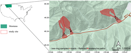
The U.S. northern Rocky Mountains of northwest Montana are classified as both coastal transition and intermountain avalanche climate (Mock and Birkeland 2000) and therefore can exhibit characteristics of both continental or coastal climates. The contrasting precipitation and temperature regimes within the region are due to the study area’s proximity to the Continental Divide, which allows both Pacific and continental air masses to influence the area’s weather. Average annual precipitation is 2,083 mm at Flattop SNOTEL (elevation 1,810 m) and peak snow water equivalent typically occurs in mid- to late April with a median value of approximately 1,100 mm (1981–2010; U.S. Department of Agriculture, Natural Resources Conservation Service 2020b). The elevation of avalanche paths within the study site ranges from approximately 1,200 to 2,200 m and covers predominantly southeast to south aspects (Table 1). Snowsheds exist at nine avalanche paths throughout JFS Canyon and at two of the three avalanche paths in this study.

Table 1. Topographic characteristics of all avalanche paths.

Path	No. of tree ring samples collected	No. of growth disturbances	Full path elevation (range) (m)	Starting zone elevation (mean) (m)	Full path slope (mean) (°)	Starting zone slope (mean) (°)	Area (km^2)	Length (m)	Vertical (m)	Median aspect (°)
Shed 10–7 (S10.7)^a	109	NA	1,233–2,193	1,910 1,964	31	35 39	0.13	1,745.66	959.74	176
1163	50	128	1,250–2,217	1,861	38	42	0.17	1,636.52	966.82	158
Shed 7 (S7)^a	46	92	1,310–2,078	1,935 1,837	29	34 36	0.57	1,686.96	768.01	152

^aTwo major starting zones for one runout.

The subalpine and montane forests are dominated by species of fir (Abies lasiocarpa, Pseudotsuga menziesii, Abies grandis), pine (Pinus ponderosa, Pinus monticola), and a mix of hemlock (Tsuga heterophylla), larch (Larix occidentalis), spruce (Picea engelmannii), cedar (Thuja plicata), birch (Betula papyrifera), and slide alder (Alnus spp.).

Lidar and spectral imagery data acquisition

We used a high point density aerial lidar data set acquired for approximately 192 km² of JFS Canyon between 20 July 2016 and 5 August 2016 (U.S. Geological Survey 2017). The longer data collection period allowed for suitable flying and data collection during leaf-on conditions. Data collection and processing adhered to a maximum nominal post spacing of 0.35 m, with a mean point density of 16 points/m².

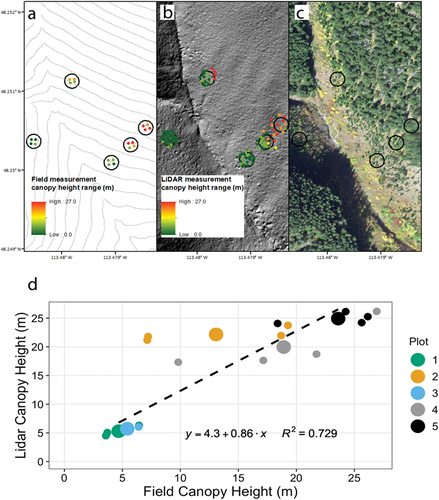
Using the approach outlined by Laes et al. (2011), we validated the lidar data by measuring tree height and diameter in July 2019 in Shed 7 using five circular field plots (plot area = 400 m²) and stratified random sampling along an elevation gradient. We did not sample vegetation types but simply used this step to field-validate canopy height values of the lidar data. However, we selected plots representative of homogenous vegetation cover in and adjacent to the avalanche path. We measured the height of the four tallest trees within each plot (n = 20 tallest trees in total) using a standard metric measuring tape and inclinometer. We included all trees whose entire or partial canopy fell within the field plot in selection of the four tallest trees. We then mapped each plot and identified the four tallest trees within each plot in the lidar data set and examined the relationship between field measurements and lidar data using the Pearson correlation coefficient.

We used aerial imagery collected by the National Agricultural Imagery Program (NAIP) for JFS Canyon in the fall of 2017 to examine spectral signatures of vegetation in avalanche paths. The four-band (red, green, blue, and near-infrared) NAIP imagery for the study site is 0.6-m horizontal spatial resolution (U.S. Department of Agriculture, Natural Resources Conservation Service 2020a).

Imagery and lidar data processing

Our vegetation mapping workflow includes multiple steps from data processing to the final vegetation classification (Figure 2). First, we clipped the lidar point data to the study area and generated a DSM for the height of vegetation using a pit-free algorithm developed by Khosravipour et al. (2014). We also created a digital terrain model (DTM) for the bare earth surface using a spatial interpolation algorithm based on nearest neighbor approach with an inverse distance weighting method. We subtracted the DTM from the DSM to produce a canopy height model (CHM) data layer.

Figure 2. General workflow of classification procedure from data processing to final vegetation classification.

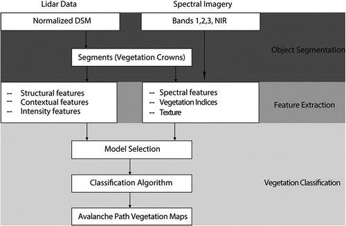
We then clipped NAIP aerial imagery to the study area and georeferenced it to align with the CHM derived from the lidar point cloud. We segmented individual tree crowns from the CHM based on the marker-controlled watershed function developed by Meyer and Beucher (1990), a common segmentation methodology for data derived from an airborne laser scanner (Hyyppä et al. 2001; Persson, Holmgren, and Soderman 2002; Solberg, Naesset, and Bollandsas 2006; Holmgren, Persson, and Soderman 2008). We clipped the resulting raster representing individual tree crowns by the extent of the three avalanche paths for this study: Shed 10–7, Path 1163, and Shed 7. We used a minimum canopy height of 0.5 m to include low-level vegetation that could provide useful information in avalanche path return period analysis. All analyses were performed using R statistical software (R Core Team 2018) using the lidR (Roussel and Auty 2019) and rLiDAR (Silva et al. 2017) packages.

Manual vegetation classification

To create an automated vegetation classification procedure using remote sensing products, we first manually classified the vegetation of a sample of objects in the imagery to create a training data set. To accomplish this, we selected 300 random individual points from the segmented lidar (CHM) data set for each avalanche path and manually classified each point to the level 1 vegetation type based on the NAIP imagery (Table 2). We only labeled objects that were clearly identifiable by vegetation type and had no confusion with other vegetation types. We included additional crown objects in object classes with low sample size (n < 30). The resultant total sample size for the crown objects increased from 300 to approximately 400 for each path. Originally, we manually identified between fifteen and nineteen vegetation classes in each avalanche path. We then progressively aggregated the classes from level 1 (all classes) to more coarse level 2 and level 3 (coarse vegetation classes) to reflect broad classes applicable to the analysis of avalanche path vegetation composition (Table 2).

Table 2. Class aggregation for avalanche path return period analysis and detailed class descriptions.

Detailed class descriptions	Level 1 All classes used in original classification	Level 2 Aggregated classes to reflect vegetation type	Level 3 Further aggregated classes relevant to avalanche path return period analysis
Subalpine fir, Douglas fir, lodgepole pine, white spruce, black spruce	Conifer no shadow, conifer with some shadow, conifer in shadow, subalpine fir, dead conifer	Coniferous forest	Mature forest
Cottonwood, birch, aspen, larch	Deciduous forest, deciduous with some shadow	Deciduous forest
Alder, false huckleberry	Green shrub, green shrub in shadow	Green shrub	Shrubland
Willow, service berry, young aspen, young cottonwood, young birch	Yellow shrub	Yellow shrub
Mountain maple, mountain ash, dogwood	Red shrub	Red shrub
Huckleberry	Huckleberry	Huckleberry
Beargrass, thimbleberry, solomon seal, grasses	Brown grassland/shrubland, off-white grassland/shrubland, green grassland/shrubland	Grassland	Grassland
Exposed rock	Grey rock outcrop, white rock outcrop	Exposed rock	Exposed rock
Seasonal snow	Snow, snow in shadow	Snow	Snow

Level 3 classes were used in our vegetation and return period analysis.

We calculated metrics commonly used to distinguish differences between tree species for each delineated tree crown object (Brandtberg et al. 2003; Holmgren and Persson 2004). These metrics can be grouped into three categories (see Table S1 for variable descriptions):

1. Structural features. We extracted the lidar-measured maximum height and crown diameter for each tree object.

2. Contextual features. Z represents the lidar-derived DTM + CHM. We calculated maximum, mean, and standard deviation of Z for each tree object as well as quantile metrics including 10th percentile, 30th percentile, 50th percentile, 70th percentile, and 90th percentile.

3. Intensity features. We calculated maximum, mean, and standard deviation of intensity for each tree object as well as intensity quantile metrics including 30th percentile, 50th percentile, 70th percentile, and 90th percentile.

We also extracted values from the spectral imagery for each lidar-derived tree crown object and grouped the metrics into the following three categories:

1. Spectral features. We extracted the mean value of all pixels within each tree crown object for bands 1, 2, 3, and 4 and used these as features.

2. Vegetation indices. We calculated the mean NDVI for each tree crown object based on the equation

(1) $\mathit{NDVI}=\frac{\left(\mathit{NIR}-\mathit{RED}\right)}{\left(\mathit{NIR}+\mathit{RED}\right)}$(1)

where NIR is the near-infrared band and RED is the red band. We calculated mean Green-Red Vegetation Index (GRVI) for each tree crown object using the equation

(2) $\mathit{GRVI}=\frac{\left(\mathit{GREEN}-\mathit{RED}\right)}{\left(\mathit{GREEN}+\mathit{RED}\right)}$(2)

• (3) Texture. We calculated NDVI variance and entropy for each tree crown object (Lillesand and Kiefer 2000).

Model selection and image classification

We grouped lidar-extracted metrics (e.g., descriptive statistics for intensity grouped together, quantile statistics for intensity grouped together) for inclusion in a model selection procedure. We used a random forest model (Breiman 2001), an ensemble learning method that can be used for image classification that operates by developing several decision trees where each node is split based on the best of a subset of predictors, for our classification procedure. We calculated the kappa value for each random forest model of all possible combinations of lidar-derived metrics as well as all possible combinations of spectral signature–derived variables. We then used the variables from the highest ranked model from both spectral signature–derived (models 1–5, see Table 3) and lidar-derived (models 6–21, see Table 3) metrics and combined them to identify the highest-ranked model for each path via model selection. Additionally, we produced models using all variables (spectral and lidar-derived variables) grouped together to compare the previous model selection against.

Table 3. Overall accuracies and kappa values for random forest models of the combinations of spectral variables and lidar variables.

	Spectral imagery variables				Lidar data features						Shed 10–7		Path 1163		Shed 7
Model	B1-B4	NDVI	GRVI	Texture	Crown height	Crown diameter	I percentile statistics	I descriptive statistics	Z percentile statistics	Z descriptive statistics	Kappa value	Overall accuracy (%)	Kappa value	Overall accuracy (%)	Kappa value	Overall accuracy (%)
1	X										0.80	83	0.75	80	0.69	74
2	X	X									0.83	86	0.76	81	0.70	74
3	X	X	X								0.85	87	0.74	79	0.71	75
4	X	X	X	X							0.87	89	0.82	86	0.80	83
5	X	X		X							0.80	83	0.84	87	0.80	83
6					X						0.17	30	0.26	41	0.37	47
7					X	X					0.25	36	0.31	44	0.37	46
8					X	X	X				0.28	39	0.27	41	0.53	60
9					X	X		X			0.47	54	0.47	56	0.60	66
10					X	X	X	X			0.47	54	0.46	56	0.68	73
11					X	X				X	0.65	70	0.61	68	0.77	80
12					X	X			X		0.60	66	0.61	69	0.74	78
13					X	X			X	X	0.62	67	0.61	69	0.74	78
14					X	X	X		X		0.62	67	0.64	71	0.77	81
15					X	X	X	X	X		0.58	64	0.66	72	0.83	86
16					X	X		X		X	0.65	70	0.63	70	0.81	84
17					X	X		X	X		0.62	68	0.66	72	0.81	84
18					X	X		X	X	X	0.65	70	0.68	74	0.81	84
19					X	X	X			X	0.63	69	0.65	72	0.78	81
20					X	X	X	X		X	0.61	67	0.65	72	0.76	80
21					X	X	X	X	X	X	0.60	66	0.69	75	0.84	87
Best spectral + Best lidar
22 (Path 10–7)	X	X	X	X	X	X		X	X	X	0.86	88
23 (Path 1163)	X	X		X	X	X	X	X	X	X			0.89	91
24 (Shed 10–7)	X	X	X	X	X	X	X	X	X	X					0.91		92
All variables
25 (Path 10–7)	X	X	X	X	X	X	X	X	X	X	0.88	90
26 (Path 1163)	X	X	X	X	X	X	X	X	X	X			0.89	91
27 (Shed 10–7)	X	X	X	X	X	X	X	X	X	X					0.91		92

Models in each category with highest kappa value were combined in best-fit model for each avalanche path. Best-fit models for each avalanche path are reported at the bottom of the table. I percentile statistics = the 10th, 30th, 50th, 70th, and 90th percentiles of intensities; I descriptive statistics = the maximum, mean, and standard deviation of intensities; Z percentile statistics = the 10th, 30th, 50th, 70th, and 90th percentiles of elevations; Z descriptive statistics = the maximum, mean, and standard deviation of the elevation. Bold indicates best-fit models for spectral imagery variables and lidar data features separately.

We trained each model on a randomly chosen subset of regions of interest (ROIs) within each avalanche path, representing approximately 50 percent of all ROIs (n ≈ 200). The remaining 50 percent of the ROIs acted as a validation subset. We selected the best performing model to predict vegetation across each avalanche path. We used the highest overall accuracy and kappa value to select the best performing model. We trained the model separately for each path due to different class prevalence between paths. We used the caret package (Kuhn et al. 2019) in R with default parameterization and 100 resampling iterations for all random forest modeling. Finally, we classified the segmented tree crown vector layer by vegetation type using the combined lidar and spectral signature best-performing model.

Dendrochronological analysis and return period reconstruction

This analysis utilizes the dendrochronology generated spatial–temporal avalanche data set by Peitzsch et al. (2019) and as presented in detail in Peitzsch et al. (2021). Briefly, our sampling strategy targeted an even number of samples collected across the path where material was available and along the avalanche path trimlines at varying elevations. Location data were not available for all samples in the Shed 10–7 path; therefore, we excluded it from this return period analysis. In Path 1163 and Shed 7 we collected a total of 96 cross sections. We sanded the samples to a fine polish to expose the anatomy of each growth ring and cross-dated cores and cross sections with each other using the skeleton plot method to account for missing and false rings (Stokes and Smiley 1996; Figure S2). We developed a site composite chronology and cross-dated with preexisting regional chronologies to confirm the exact calendar dating of each tree ring (International Tree Ring Data Bank 2020) using the dating quality control software COFECHA (Holmes 1983; Grissino-Mayer 2001). For further details on cross-dating methods and accuracy calculation for this data set, see Peitzsch et al. (2019).

We compiled a data set of the full spatial extent of individual avalanche events from a combination of tree ring samples (period of record: 1936–2017) and recent historical observations (period of record: 2000–2021). Since 2000, observational records of avalanches in these paths were substantially more detailed than those prior to 2000 and included a thorough description, images, and occasionally fracture line and debris deposit measurements. The dendrochronology samples have a much longer record but can underestimate avalanche activity in a single path (Corona et al. 2012). Therefore, we combined observational and dendrochronological data for a more robust data set for our return period analysis.

We determined the extent of each avalanche using the spatial patterns of tree ring samples exhibiting avalanche disturbance signals for any given year and field notes and images from the BNSF Avalanche Program (BNSF 2021). For every year an avalanche occurred in each path, we manually digitized the extent using ArcGIS 10.6.1 (ESRI 2021) to also include all avalanche events present in the dendrochronology samples for the corresponding year. We then converted the manually digitized vector polygon to a raster and assigned a value of 1 to all area included in the avalanche extent raster for each year. This resulted in a binary value (1 = avalanche, 0 = no avalanche) for any pixel within the avalanche event extents for every year in the period of record. We then used these values to estimate spatially explicit return periods for Path 1163 and Shed 7 using methods developed by Meseșan, Gavrilă, and Pop (2018). For each pixel within each avalanche path, we calculated the return period (RP) using:

(3) $\mathit{RP}=\frac{Y_r}{W_n}$(3)

where $Y_r$ is the number of years in the period of record, or full chronology, based on the age of each tree or the observational record at each pixel and $W_n$ is the number of winters an avalanche was recorded in the tree ring or observed record.

We used the Intersection tool in ArcGIS to intersect the vegetation classification vector layers with the return period layers to calculate the proportion of each vegetation classification for each return period. We then examined lidar-derived tree height differences in three commonly used return period intervals (one to three years, four to ten years, and eleven to thirty years; Canadian Avalanche Association [CAA] 2016). We used analysis of variance and Tukey’s honestly significant difference test test to compare tree height between the three return interval categories (Devore and Peck 2005).

Finally, to gain insight into spatial extents of return periods beyond the areas we covered using observational and dendrochronological data, we used tree stand age as a proxy for return periods. To do this, we used lidar height data and calculated tree stand age based on the linear relationship developed by Racine et al. (2014) and applied it to individual conifers in our vegetation classification maps of each path. The linear model used is

(4) $\mathit{age}=\mathit{\beta }0+\mathit{\beta }1\ast \mathit{H}$(4)

where age is mean plot age, H is the canopy height, and β0 and β1 are the parameters estimated by mean square error minimization and are 4.40 and 3.16, respectively. We applied the linear relationship to our study area using a 11.28-m moving window to match the plot size of Racine et al. (2014). We then binned estimated tree stand age values into four return interval categories (0–22 years, 23–50 years, 51–75 years, 76–100 years).

Results

Lidar field validation

Comparing the mean in situ canopy height field-based measurements against the mean lidar canopy height measurements for each of the five plots yielded reasonably matched distributions and plot means that were strongly related (R² = 0.729; Figure 3 and Table S2).

Figure 3. Example canopy height measurements from Shed 7. (a) In situ height measurements (m) of the four tallest trees in each field plot (open black circles). Contour lines represent 10-m elevation intervals. (b) Field plots with lidar measurements (m) for each plot. Note that samples outside the plots were considered in the validation procedure because their canopy extended over the plot area. (c) Field plots with the spectral imagery. (d) Relationship of measured mean height within each field plot (x-axis) against the lidar canopy height (y-axis). Colors represent the five field plots, and the larger dots symbolize the mean height for each plot. The dashed line is the linear regression line of all points (not including the mean values for each plot).

Manually classified objects (ROI)

Each avalanche path contains a unique combination of specific avalanche vegetation classes. We attempted to manually identify similar amounts of each vegetation class within each path. Given the lack of some classes in each path, the number of manually identified classes varies (Table 4).

Table 4. The number of objects (points) manually identified in each vegetation class within each avalanche path.

ROIs in each vegetation class
Level 1 vegetation class	Path 10.7	Path 1163	Shed 10-7	Level 3 vegetation class	% of total objects
Conifer no shadow	27	31	15	Mature forest	41
Conifer with some shadow	55	50	20
Conifer in shadow	16	29	7
Subalpine fir	n/a	n/a	26
Dead conifer	8	8	17
Deciduous forest	34	31	49
Deciduous with some shadow	27	12	n/a
Green shrub	30	n/a	18	Shrubland	22
Green shrub in shadow	n/a	n/a	19
Yellow shrub	35	33	20
Red shrub	33	20	23
Huckleberry	n/a	n/a	18
Brown grassland/shrubland	29	28	11	Grassland	17
Off-white grassland/shrubland	40	37	23
Green grassland/shrubland	n/a	21	n/a
Grey rock outcrop	n/a	19	n/a	Exposed rock	10
White rock outcrop	40	34	19
Snow	26	27	6	Snow	10
Snow in shadow	10	10	29
Total	410	390	320		100

n/a indicates classes not present in corresponding classification.

Random forest model classification

We calculated accuracy statistics following aggregation to level 2 vegetation classes (Table 2). Accuracy results reflect the ability of the random forest model to automate vegetation classification against our manually identified vegetation classification. The importance of each variable is different for each path (Figure 4). For Shed 10–7, models 4 and 18 had the highest-ranking kappa value based on the spectral and lidar data sets, respectively (Table 3). Vegetation predicted across Shed 10–7 based on these two combined models resulted in an overall accuracy of 88 percent (kappa = 0.86). For Path 1163, models 5 and 21 had the highest-ranking kappa values and, when combined, resulted in an overall accuracy of 91 percent (kappa = 0.89). For Shed 7, models 4 and 21 had the highest-ranking kappa value and when combined resulted in an overall accuracy of 92 percent (kappa = 0.91).

Figure 4. The variable importance plots rank the relative importance for each variable in the best-performing random forest models (see Table 3) for (a) model 25 (Shed 10–7), (b) model 26 (Path 1163), and (c) model 27 (Shed 7). See Table S2 for variable descriptions.

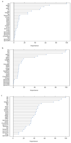
When applying the random forest model for each path using all variables, the overall accuracies and kappa values remained the same for Path 1163 and Shed 7. However, the overall accuracy of Shed 10–7 increased from 88 percent (kappa = 0.86) to 90 percent (kappa = 0.88). Therefore, we used models with all variables (models 25, 26, and 27) for the final vegetation classifications. These three models yielded the highest overall accuracy across each of the three paths. The most important variables for the final models used to classify vegetation in each path were B3 (spectral band green) for Shed 10–7 and Path 1163 and B2 (spectral band blue) for Shed 7 (Figure 4).

In all three avalanche paths, classifications exhibited minor confusion between deciduous forest and coniferous forest classes (Table 5 and Figure 5). In Shed 10–7 and Shed 7, there was confusion among grassland, green shrub, yellow shrub, and red shrub, as well as confusion between deciduous forest and yellow shrub. In Shed 10–7 there was minor confusion between coniferous forest and green shrub and coniferous forest and snow. In Path 1163, rock outcrop was confused with snow.

Figure 5. Modeled labeled vegetation (level 2 classes; see Table 2) mapping results for Shed 10–7, Path 1163, and Shed 7 using a combination of spectral and lidar data. The avalanche paths are outlined with a 50-m buffer (black polygons) for context of surrounding vegetation. Note that these three paths are not all adjacent to each other (Figure 1).

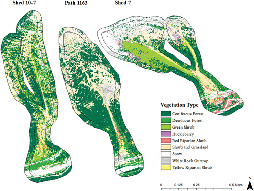
Table 5. Confusion matrices associated with the best-performing model for each individual avalanche path.

		Grassland	Coniferous forest	Deciduous forest	Snow	Green shrub	Huckleberry	Red shrub	Exposed rock	Yellow shrub	Producer accuracy (%)
Shed 10-7
Grassland		15	1	0	0	0	~	2	0	0	83
Coniferous forest		0	40	0	0	1	~	0	0	0	98
Deciduous forest		1	2	34	0	0	~	0	0	0	92
Snow		0	2	0	15	0	~	0	1	0	83
Green shrub		2	2	0	0	13	~	0	0	0	76
Huckleberry		~	~	~	~	~	~	~	~	~	~
Red shrub		1	0	0	0	0	~	15	0	1	88
Exposed rock		0	0	0	0	0	~	0	21	0	100
Yellow shrub		0	0	2	0	0	~	0	0	12	86
User accuracy (%)		79	85	94	100	93	~	88	95	92	90
Path 1163
Grassland		29	0	0	0	~	~	0	0	1	97
Coniferous forest		1	55	1	0	~	~	0	0	0	96
Deciduous forest		0	2	21	0	~	~	0	0	1	88
Snow		0	0	0	14	~	~	0	6	0	70
Green shrub		~	~	~	~	~	~	~	~	~	~
Huckleberry		~	~	~	~	~	~	~	~	~	~
Red shrub		1	0	0	0	~	~	8	0	0	89
Exposed rock		0	0	0	1	~	~	0	17	0	94
Yellow shrub		1	0	0	0	~	~	0	0	15	94
User accuracy (%)		91	96	95	93	~	~	100	74	88	91
Shed 7
Grassland		19	0	0	0	0	0	0	0	2	90
Coniferous forest		0	67	0	0	1	0	0	0	0	99
Deciduous forest		0	5	39	0	0	0	0	0	0	89
Snow		0	0	0	13	0	0	0	0	0	100
Green shrub		0	0	0	0	34	1	0	0	0	97
Huckleberry		1	0	0	0	0	9	0	0	0	90
Red shrub		3	0	0	0	0	0	8	0	2	62
Exposed rock		0	0	0	0	0	0	0	28	0	100
Yellow shrub		2	0	2	0	0	0	0	1	17	77
User accuracy (%)		76	93	95	100	97	90	100	97	81	92

Actual classifications are in the right column and predicted values are in the bottom row for each path. Confusion matrices for the best-performing spectral and lidar models can be found in Tables S3 and S4.

Combining lidar and spectral imagery to automate species-level vegetation classification yielded high overall accuracy for all three avalanche paths when compared to the manual classification of vegetation within avalanche paths using aerial imagery. In Path 1163 and Shed 7, combining all spectral and lidar-derived variables represents a substantial improvement in overall accuracy from using spectral imagery alone (+4 percent and +9 percent, respectively) and from lidar data alone (+16 percent and +5 percent, respectively) in the ability to map vegetation within avalanche paths (Table 6). In Shed 10–7, combining all spectral and lidar-derived variables resulted in an increase in overall accuracy of +1 percent (within 95 percent confidence intervals) when compared to overall accuracy obtained from spectral imagery alone and an increase of +20 percent compared to overall accuracy obtained from lidar-derived variables.

Table 6. Classification accuracies for each avalanche path using different variables or combinations of variables.

	1. Spectral		2. Lidar		3. Combined (1 + 2)		4. All variables
Path	Kappa value	Overall accuracy (%)	Kappa value	Overall accuracy (%)	Kappa value	Overall accuracy (%)	Kappa value	Overall accuracy (%)
Shed 10–7	0.87	89	0.65	70	0.86	88	0.88	90
Path 1163	0.84	87	0.69	75	0.89	91	0.89	91
Shed 7	0.80	83	0.84	87	0.91	92	0.91	92

See Table 4 for variables included in each model. See Tables S3 and S4 for confusion matrices on best-performing spectral and lidar models.

Return period vegetation

The return period results from the delineated avalanche paths for Path 1163 and Shed 7 suggest minimum return periods of 1.2 years and 2.4 years, respectively (Figure 6). The mapped return periods generally follow the slope morphology with higher frequency return periods centered around the incised channel and higher in elevation, with frequency decreasing along the vertical extent of the slope for both avalanche paths. For Shed 7, return periods for a corner of the southwest portion of the path are of relatively high frequency although no longer associated with the incised channel. As noted from photographic evidence, large avalanches flow over the top of the snow shed and end in a slight curve to this corner.

Figure 6. (a,c) Mapped return periods and (b,d) random forest model–generated vegetation classes for return interval zones for (a,b) Shed 7 and (c,d) Path 1163. The orange lines represent contour lines spaced at 10-m intervals to illustrate topography changes.

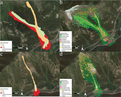
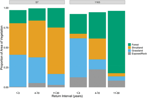
The proportion of vegetation classes within the return period intervals for Path 1163 follows a pattern where proportion of shrubland and grassland is greater in areas of higher frequency avalanche activity and the proportion of forest is greater in areas of lower frequency (Figure 7). However, in Path 1163, the high frequency interval locations are comprised of greater proportions of forest when compared to similar return intervals in Shed 7. Shed 7 also contains substantially more shrubland and grassland than Path 1163 throughout the larger return intervals, specifically the eleven- to thirty-year interval.

Figure 7. Proportions of each vegetation class for Shed 7 (left) and Path 1163 (right). Return interval years are represented on the x-axis. Vegetation classes are represented by color (legend on right). Note that columns do not necessarily sum to 1.0 because of classification of perennial snow in the data set.

Return period and vegetation height

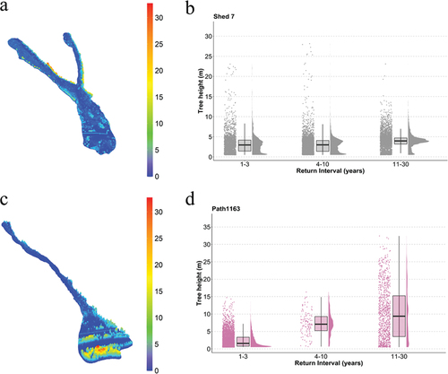
Next, we examined the relationship between lidar derived vegetation height and categorical return periods. Using analysis of variance, we found a statistically significant difference in mean tree height by return period interval for both Shed 7, F(2) = 171.3, p < .001, and Path 1163, F(2) = 1518, p < .001 (Figure 8). Tukey’s post hoc test revealed that tree height is, on average, greatest in the eleven- to thirty-year return interval category (4.06 m) in Shed 7 but slightly and significantly lower in the four- to ten-year interval category (3.10 m) when compared to the one- to three-year return interval (3.27 m; p = .01; Figure 8b). In Path 1163, tree height is, on average, greater in each successively larger return period interval category (one- to three-year = 2.40 m; four- to ten-year = 7.30 m; eleven- to thirty-year = 10.10 m; Figure 8d).

Figure 8. (a,c) Lidar-derived heights of vegetation and (b,d) raincloud plots (b,d) of tree height (m) for return intervals for (a,b) Shed 7 and (c, d) Path 1163. Raincloud plots show the individual return intervals (years) and associated tree height for each tree (points on left), box plots (center) showing the median (black horizontal line) and interquartile ranges for heights for each return interval bin, and the distribution of tree heights for each bin (shaded distribution on right). All pairwise comparisons of return intervals are significantly different in both Shed 7 and Path 1163.

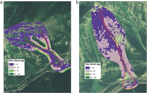
Finally, to gain insight into tree stand age as a proxy for return periods beyond our available observational and dendrochronological data, we used the lidar canopy height to estimate stand age. We found tree stands in the furthest reaches and beyond the outlined paths to reach 80 to 100 years of age (Figure 9). There are areas with no data classified as forest in parts of the runout zone in each path due to infrastructure such as roads and railways.

Figure 9. Tree stand age for (a) Shed 7 and (b) Path 1163. The red outline depicts the general outline of the avalanche path. The areas without color associated with a tree stand age represent areas without vegetation classified as forested areas in this study (see Figure 6 for classification).

Discussion

Vegetation classification

Using lidar and spectral imagery products to estimate avalanche path vegetation classes appears promising. The strong correlation between lidar canopy height and field-measured canopy height suggests that lidar estimates are suitable for vegetation class modeling. Slight differences between the measured and lidar height data sets can be attributed to using plot mean height values instead of comparing individual tree heights from one data set to another. Comparing individual tree heights between data sets would require centimeter-level resolution for each data set, and the lidar data have a minimum horizontal resolution of 0.5 m. Field measurement error could also be a source of error given the steep terrain associated with the plots.

For all paths, we used the best-performing random forest model with all spectral and lidar-derived variables. However, in the interest of experimenting with a less complex model, for Shed 7 we manually omitted elevation and intensity quantile statistics and maximum values, resulting in a decrease of approximately −2 percent overall accuracy for Shed 7 when compared to the full best-fit random forest model. This suggests that the full suite of metrics used for the best-performing model is necessary to obtain higher accuracy for vegetation modeling in avalanche paths. Accordingly, we did not run a random forest model for all permutations of variables because of the increase in accuracy as variables were added to each model.

Avalanche activity within the study area capable of destroying trees and changing vegetation patterns between the summer of lidar data collection and field sampling could impact the labeling of training and validation tree crowns, because we delineated crowns from the lidar data but manually classified vegetation based on NAIP imagery. For example, it is possible that a tree crown that existed in 2016 no longer existed in 2017, resulting in a polygon manually classified with spectral attributes but with physical variables related to the previous landcover (i.e., an ROI labeled grassland in 2017 imagery was a coniferous tree in 2016 with associated canopy variables). This could be one source of confusion between classes and could have negatively impacted overall accuracy values.

The starting zones of each avalanche path are characterized by predominantly grassland and rock outcrop except for Shed 10–7, which is characterized by grassland and coniferous forest. The coniferous forest in Shed 10–7 generally comprises small trees characteristic of treeline forests. One possible explanation for this is that Shed 10–7 is dominated by vegetation classes easily distinguishable by spectral variables (e.g., coniferous forest and senesced grassland) and as a result does not rely as heavily on variables such as canopy height or that in some classes (e.g., coniferous forest) the age of vegetation varies greatly and was not completely captured when we developed our regions of interest. Using Ikonos satellite imagery in the same study area as ours, Walsh et al. (2004) found higher greenness levels at higher elevations, suggesting the presence of mixed shrubs and herbaceous material, and lower greenness levels at lower elevations where the accumulation of debris piles and other downed and scoured materials may exist. Our results suggest that vegetation patterns along an elevational gradient within an avalanche path are more complex than a simple pattern with smaller, herbaceous vegetation near the starting zones and larger trees near the runout zones.

Vegetation patterns across a lateral transect indicate shrub or grasslands associated with incised stream channels in all three avalanche paths. Similarly, Walsh et al. (2004) found a decrease in greenness away from the center of the avalanche track, indicating more herbaceous shrubs in the center of the paths and larger trees toward the trimlines of the avalanche paths. However, the lateral composition of vegetation also varies along an elevational gradient despite the strong signal of grassland in the incised channel. In other words, the vegetation along the flanks adjacent to the incised channel zone is not consistent up and down the avalanche paths. This coincides with earlier work by Malanson and Butler (1986) and Erschbamer (1989).

Return period intervals and vegetation characteristics

The return periods depicted here are likely underestimations given the limitation of dendrochronological techniques in developing an avalanche chronology (Corona et al. 2012), particularly in locations where few samples exist (e.g., the incised channel on the avalanche paths), as well as an incomplete observational record further back in time. Therefore, the absolute values of the return periods should be used with caution, and the patterns of return periods are the more critical component to this analysis.

The location in Shed 7 where the highest frequency band continues into the southwest sector of the path is likely due to a substantial decrease in slope angle and more uniform planar slope. The stream channel is not as deep at this location, potentially allowing avalanche debris to disperse laterally. This is also the point of deceleration and eventual stopping point as it nears the theoretical alpha angle (Lied and Bakkehøi 1980; Mears 1989).

For Shed 7, locations with higher frequency avalanche activity within the mapped area are characterized predominantly by grassland and shrubland, which are mostly shade-intolerant species, and this is consistent with previous work (Butler 1979). For Path 1163, the zone with the highest frequency return period consists of predominantly grassland, and greater return periods consist of a mix of shrubland, grassland, and forest. This avalanche path is steep and narrow, with a constriction approximately two-thirds down the avalanche path from the top. Thus, very frequent avalanches are likely to follow the incised channel but avalanches greater than the three-year frequency zone appear to spread more laterally across the lower track and runout zone. In Path 1163, the proportion of forest in the most frequent return periods zones is likely attributable to the influence of the incised channel constraining avalanche flow to a certain level within the path or the ability of small to moderate-sized trees to withstand avalanche impact. These trees may be young but large enough to be characterized as coniferous forest in the vegetation classification (Kajimoto et al. 2004).

Differences in vegetation within the specific return periods for Path 1163 and Shed 7 are due to the geomorphology of each slope. Path 1163 has a smaller and narrower starting zone and is further constrained by the narrow, incised channel of the track. This causes all of the return periods within the path to be laterally narrower when compared to Shed 7, with potentially more overlap. Shed 7, on the other hand, has a wide starting zone and track and is, overall, less steep than Path 1163. This allows avalanches to disperse more easily, thereby causing a greater proportion of each return period to harbor grassland and shrubland vegetation classes and a greater proportion of forest in the eleven- to thirty-year return interval in Path 1163.

It could be useful to train a vegetation model on one or several avalanche paths to be able to predict across other avalanche paths where return period data are nonexistent. However, our results suggest that doing so would be potentially inaccurate because of the variable vegetation classes and patterns across any given path. The increasingly greater proportion of forest in larger return interval categories across paths suggests that using evidence of more forested terrain to categorize less frequent categorical return intervals is feasible. Therefore, to extrapolate specific return period intervals based on all vegetation classes across a large area using a lidar- and spectrally derived vegetation model would require a larger training data set from a wide variety of heterogenous avalanche paths and a very large tree ring reconstructed return period interval data set or a long observational record. This was not possible in this study because lidar data are not available for all of the avalanche paths in the tree ring data set (Peitzsch et al. 2019) we used in this study.

Return period intervals and lidar-derived tree height

We examined classifying the return period zones based solely on lidar-derived canopy height to identify whether any nuances in adjacent return period zones exist. We found, on average, statistically significant differences in mean tree height between return period categories. The lowest frequency return period zones in both avalanche paths are characterized by the greatest vegetation height, as expected, but are still prone to impact from larger avalanches (Teich et al. 2012). Therefore, investigating patterns in canopy height alone was useful in examining return interval categories. However, our results suggest that vegetation height does not necessarily increase linearly with return intervals. For example, in Shed 7, vegetation height located in the most frequent return interval category (one- to three-year) is, on average, slightly greater than the four- to ten-year return interval. This difference could potentially be attributed to different frequencies in the two main starting zones of Shed 7. In other words, the eastern starting zone in Shed 7 avalanches more frequently and the runout of the one- to three-year return period zone (below the confluence of the two starting zones) consists of taller vegetation than the starting zones. Therefore, this may lead to the inclusion of taller vegetation in the one- to three-year return period for this particular avalanche path. However, the low frequency return interval category (eleven- to thirty-year) in each path was characterized by the highest canopy height.

Additionally, by examining stand age as a proxy for return intervals beyond our dendrochronological or observational record, we found distinct canopy height values associated with the oldest stand age located in the furthest reaches of the runout zone and well outside the lateral extent of the identified avalanche path. This suggests that lidar-derived canopy height can potentially be used to identify return period categories commonly used in planning and to examine stand age as a proxy for categorical return intervals in areas with distinct vegetation height differences. However, caution should be used when evaluating this metric for detailed infrastructure planning purposes, and the metric should be used in combination with other tools.

Implications

In many applications of avalanche risk management, an assessment needs to be made regarding how to implement measures to mitigate the avalanche risk. Thresholds of avalanche size and/or impact pressure, in combination with categorical return periods, are often used to guide this process. For example, for terrain assessment (e.g., Avalanche Terrain Exposure Scale; Statham, McMahon, and Tomm 2006; Larsen et al. 2020), the one- to thirty-year return period for events size D2 or greater is used as one of the thresholds for “simple” avalanche terrain. Likewise, for assessments of specific elements at risk (e.g., for roads with low traffic exposure and/or low opportunity costs), the CAA (2016) suggests that events size D3 or greater should have a typical return period of thirty years or less and events size D2 or greater should have a typical return period of ten years or less. Furthermore, for hazard zoning applications in Canada for occupied structures, a thirty-year return period combined with estimated impact pressures is used to differentiate between red, white, and blue zones (McClung 2005; CAA 2016).

In the absence of a robust observational record, return period assessments can be made, in part, based on vegetation evidence. In these cases, and depending on the scale and type of assessment, it is not uncommon to have limited dendrochronological observations from some paths and extrapolate these data to adjacent paths. Our analysis highlights the potential pitfalls in taking this approach, especially when applied to high frequency events less than ten years. This suggests that these extrapolations will likely have a high degree of uncertainty and should only be attempted for return periods of eleven to thirty years or greater and that even then there is likely to be some degree of variability between avalanche paths.

Limitations

We recognize that the vegetation composition of the avalanche paths is only representative of the time when data were collected. Timing of data acquisition, often a factor of data availability, can impact classification accuracy in the event of disturbances such as avalanches around the time of data collection. In this study, lidar data were collected in July to August 2016. In the absence of NAIP imagery collected in 2016, we chose to work with 2017 NAIP imagery due to its unusually late collection date (September/October) and therefore unique ability to aid in differentiating between species groups that at other times of the year would have similar spectral signatures. The coarse resolution (30 m) of Landsat data (though available semi-monthly) would negate the utility of the high-resolution (crown-level) lidar data set. Another limitation is the underestimation that using dendrochronological techniques can yield in terms of avalanche frequency. The proportions of vegetation classes within return period zones would potentially change if avalanche return periods were more frequent. Additionally, we show that vegetation composition exerts a substantial effect on being able to classify return intervals across multiple avalanche paths even in our study area with similar aspect and elevation. Therefore, extrapolating return intervals based on vegetation characteristics may only be appropriate in other regions if vegetation patterns are similar across avalanche paths.

Conclusions

In this study, we implemented a novel approach using lidar, aerial imagery, and a random forest model to classify vegetation within avalanche paths. We then used dendrochronological techniques and a twenty-year historical avalanche occurrence data set combined with spatial interpolation to calculate and map avalanche return periods and characterize the vegetation within those return period zones. Our results suggest that the combination of lidar and spectral signature metrics provides the best accuracy for predicting vegetation classes within complex avalanche terrain rather than lidar or spectral signatures alone. The zones with highest frequency return periods were broadly characterized by grassland and shrubland, but topography greatly influences the vegetation classes as well as the return periods. Lidar-derived canopy height also shows promise in distinguishing categorical return periods, but nuances within each path exist. Overall, the ability to characterize vegetation within various avalanche return period zones using remote sensing data provides land use planners and avalanche forecasters a tool for assessing return periods and the ecological effects of large-magnitude avalanche events.

Disclaimer

Any use of trade, firm, or product names is for descriptive purposes only and does not imply endorsement by the U.S. Government.

Acknowledgments

The U.S. Geological Survey Ecosystems Climate R&D provided funding for this project. Caitlyn Florentine and Zachary Miller assisted with fieldwork. Richard Steiner and Adam Clark with Hamre and Associates provided publicly available avalanche occurrence data (BNSF 2021).

Disclosure statement

No potential conflict of interest was reported by the author(s).

Supplementary material

Supplemental data for this article can be accessed online at https://doi.org/10.1080/15230430.2024.2310333

Additional information

Funding

This work was supported by the U.S. Geological Survey - Ecosystems, Climate Research and Development Program.

References

- Bartelt, P., and V. Stockli. 2001. The influence of tree and branch fracture, overturning and debris entrainment on snow avalanche flow. Annals of Glaciology 32: 209–22. doi:10.3189/172756401781819544.
- Bebi, P., D. Kulakowski, and C. Rixen. 2009. Snow avalanche disturbances in forest ecosystems-state of research and implications for management. Forest Ecology and Management 257, no. 9: 1883–92.
- Brandtberg, T., T. A. Warner, R. E. Landenberger, and J. B. McGraw. 2003. Detection and analysis of individual leaf-off tree crowns in small footprint, high sampling density lidar data from the eastern deciduous forest in North America. Remote Sensing of Environment 85, no. 3: 290–303. doi:10.1016/S0034-4257(03)00008-7.
- Breiman, L. 2001. Random forests. Machine Learning 45: 5–32. doi:10.1023/A:1010933404324.
- Brožová, N., J.-T. Fischer, Y. Bühler, P. Bartelt, and P. Bebi. 2020. Determining forest parameters for avalanche simulation using remote sensing data. Cold Regions Science and Technology, 172: 102976. doi:10.1016/j.coldregions.2019.102976.
- Bühler, Y., D. von Rickenbach, A. Stoffel, S. Margreth, L. Stoffel, and M. Christen. 2018. Automated snow avalanche release area delineation – Validation of existing algorithms and proposition of a new object-based approach for large-scale hazard indication mapping. Natural Hazards and Earth System Sciences 18, no. 12: 3235–51. doi:10.5194/nhess-18-3235-2018.
- Burlington Northern Santa Fe Avalanche Safety Program. 2021. Avalanche Alley: Avalanche and weather data in John F. Stevens Canyon, Montana. https://avalanchealley.com.
- Burrows, C. J., and V. L. Burrows. 1976. Procedures for the study of snow avalanche chronology using growth layers of woody plants. Occasional Paper No. 23. Boulder: Institute of Arctic and Alpine Research, Universtiy of Colorado.
- Butler, D. R. 1979. Snow avalanche path terrain and vegetation, Glacier National Park, Montana. Arctic and Alpine Research 11, no. 1: 17–32. doi:10.2307/1550456.
- Butler, D. R., and G. P. Malanson. 1985. A history of high-magnitude snow avalanches, southern Glacier National Park, Montana, U.S.A. Mountain Research and Development 5, no. 2: 175–82. doi:10.2307/3673256.
- Canadian Avalanche Association. 2016. Technical aspects of snow avalanche risk management ─ resources and guidelines for avalanche practitioners in Canada, eds. C. Campbell, S. Conger, B. Gould, P. Haegeli, B. Jamieson, and G. Statham. Revelstoke, BC: Canadian Avalanche Association.
- Corona, C., J. Lopez Saez, M. Stoffel, M. Bonnefoy, D. Richard, L. Astrade, and F. Berger. 2012. How much of the real avalanche activity can be captured with tree rings? An evaluation of classic dendrogeomorphic approaches and comparison with historical archives. Cold Regions Science and Technology 74–75: 31–42. doi:10.1016/j.coldregions.2012.01.003.
- Devore, J., and R. Peck. 2005. Statistics - the exploration and analysis of data, 766. Belmont: Brooks/ Cole.
- Dubayah, R. O., and J. B. Drake. 2000. Lidar remote sensing for forestry. Journal of Forestry 98, no. 6: 44–6.
- Erschbamer, B. 1989. Vegetation on avalanche paths in the Alps. Vegetatio 80: 139–46. doi:10.1007/BF00048037.
- ESRI. 2021. ArcGIS. 10.6.1. Redlands, CA: Environmental Systems Research Institute.
- Feistl, T., P. Bebi, and P. Bartelt. 2013. The role of slope angle, ground roughness and stauchwall strength in the formation of glide-snow avalanches in forest gaps. In Proceedings of the 2013 international snow science workshop, ed. F. Naaim-Bouvet, Y. Durand, and R. Lambert, 760–5. Grenoble, France.
- Feistl, T., P. Bebi, M. Teich, Y. Buhler, M. Christen, K. Thuro, and P. Bartelt. 2014. Observations and modeling of the braking effect of forests on small and medium avalanches. Journal of Glaciology 60, no. 219: 124–38. doi:10.3189/2014JoG13J055.
- Gaume, J., J. Schweizer, A. Herwijnen, G. Chambon, B. Reuter, N. Eckert, and M. Naaim. 2014. Evaluation of slope stability with respect to snowpack spatial variability. Journal of Geophysical Research: Earth Surface 119, no. 9: 1783–99.
- Grissino-Mayer, H. 2001. Evaluating crossdating accuracy: A manual and tutorial for the computer program COFECHA. Tree-Ring Research 57, no. 2: 205–21.
- Hesdstrom, N. R., and J. W. Pomeroy. 1998. Measurements and modelling of snow interception in the boreal forest. Hydrological Processes 12: 1611–25. doi:10.1002/(SICI)1099-1085(199808/09)12:10/11<1611::AID-HYP684>3.0.CO;2-4.
- Holmes, R. L. 1983. Analysis of tree rings and fire scars to establish fire history. Tree-Ring Bulletin 43: 51–67.
- Holmgren, J., and A. Persson. 2004. Identifying species of individual trees using airborne laser scanner. Remote Sensing of Environment 90, no. 4: 415–23. doi:10.1016/S0034-4257(03)00140-8.
- Holmgren, J., A. Persson, and U. Soderman. 2008. Species identification of individual trees by combining high resolution LIDAR data with multi-spectral images. International Journal of Remote Sensing 29, no. 5: 1537–52. doi:10.1080/01431160701736471.
- Hyyppä, J., O. Kelle, M. Lehikoinen, and M. A. Inkinen. 2001. A segmentation-based method to retrieve stem volume estimates from 3-D tree height models produced by laser scanners. IEEE Transactions on Geoscience and Remote Sensing 39: 969–75.
- International Tree Ring Data Bank. 2020. International Tree Ring Data Bank (ITRDB). https://www.ncei.noaa.gov/products/paleoclimatology/tree-ring.
- Johnson, E. A. 1987. The relative importance of snow avalanche disturbance and thinning on canopy plant popluations. Ecology 68, no. 1: 43–53. doi:10.2307/1938803.
- Kajimoto, T., H. Daimaru, T. Okamoto, T. Otani, and H. Onodera. 2004. Effects of snow avalanche disturbance on regeneration of subalpine Abies mariesii forest, Northern Japan. Arctic, Antarctic, and Alpine Research 36, no. 4: 436–554. doi:10.1657/1523-0430(2004)036[0436:EOSADO]2.0.CO;2.
- Khosravipour, A., A. K. Skidmore, M. Isenburg, T. J. Wang, and Y. A. Hussin. 2014. Generating Pit-free Canopy height models from airborne lidar. Photogrammetric Engineering & Remote Sensing 80, no. 9: 863–72. doi:10.14358/PERS.80.9.863.
- Krajick, K. 1998. Animals thrive in an avalanche’s wake. Science 279, no. 5358: 11853. doi:10.1126/science.279.5358.1853.
- Kuhn, M., J. Wing, S. Weston, A. Williams, C. Keefer, A. Engelhardt, T. Cooper, et al., 2019. caret: Classification and regression training. R package version 6.0-84. https://CRAN.R-project.org/package=caret.
- Kulakowski, D., C. Rixen, and P. Bebi. 2006. Changes in forest structure and in the relative importance of climatic stress as a result of suppression of avalanche disturbances. Forest Ecology and Management 223: 66–74. doi:10.1016/j.foreco.2005.10.058.
- Laes, D., S. E. Reutebuch, R. J. McGaughey, and B. Metchell. 2011. Guidelines to estimate forest inventory parameters from lidar and field plot data. U.S. Forest Service.
- Larsen, H. T., J. Hendrikx, M. S. Slåtten, and R. V. Engeset. 2020. Developing nationwide avalanche terrain maps for Norway. Natural Hazards 103, no. 3: 2829–47. doi:10.1007/s11069-020-04104-7.
- Leitinger, G., P. Höller, E. Tasser, J. Walde, and U. Tappeiner. 2008. Development and validation of a spatial snow-glide model. Ecological Modelling 211, no. 3–4: 363–74. doi:10.1016/j.ecolmodel.2007.09.015.
- Lied, K., and K. Bakkehøi. 1980. Empirical calculations of snow-avalanche run-out distance based on topographic parameters. Journal of Glaciology 26, no. 94: 165–77. doi:10.3189/S0022143000010704.
- Lillesand, T. M., and R. W. Kiefer. 2000. Remote sensing and image interpretation. Vol. 4. New York, NY: Wiley & Sons.
- Mace, R. D., and J. S. Waller. 1997. Spatial and temporal interaction of male and female grizzly bears in Northwestern Montana. Journal of Wildlife Management 61, no. 1: 39–52. doi:10.2307/3802412.
- Malanson, G. P., and D. R. Butler. 1984. Transverse pattern of vegetation on avalanche paths in the northern Rocky Mountains, Montana. Great Basin Naturalist 44, no. 3: 453–7.
- Malanson, G. P., and D. R. Butler. 1986. Floristic patterns on avalanche paths in the Northern Rocky Mountains, USA. Physical Geography 7, no. 3: 231–8. doi:10.1080/02723646.1986.10642293.
- McClung, D. M. 2005. Risk-based definition of zones for land-use planning in snow avalanche terrain. Canadian Geotechnical Journal 42, no. 4: 1030–8. doi:10.1139/t05-041.
- McClung, D. M., and P. Schaerer. 2006. The avalanche handbook. Seattle, WA: Mountaineers Books.
- McCollister, C. M., R. H. Comey. 2009. Using LiDAR (Light distancing and ranging) data to more accurately describe avalanche terrain. In Proceedings of the 2009 International Snow Science Workshop, ed. J. Schweizer and A. van Herwijnen, 463–7, September 27–October 2. Davos, Switzerland.
- Mears, A. I. 1989. Regional comparisons of avalanche-profile and runout data. Arctic and Alpine Research 21, no. 3: 283–7. doi:10.2307/1551567.
- Meseșan, F., I. G. Gavrilă, and O. T. Pop. 2018. Calculating snow-avalanche return period from tree-ring data. Natural Hazards 94, no. 3: 1081–98. doi:10.1007/s11069-018-3457-y.
- Meyer, F., and S. Beucher. 1990. Morphological segmentation. Journal of Visual Communication and Image Representation 1, no. 1: 21–46. doi:10.1016/1047-3203(90)90014-M.
- Mock, C. J., and K. W. Birkeland. 2000. Snow avalanche climatology of the western United States mountain ranges. Bulletin of the American Meteorological Society 81, no. 10: 2367–92. doi:10.1175/1520-0477(2000)081<2367:SACOTW>2.3.CO;2.
- Molotch, N., P. Blanken, M. Williams, A. Turnipseed, R. Monson, and S. Margulis. 2007. Estimating sublimation of intercepted and sub-canopy snow using eddy covariance systems. Hydrological Processes 21: 1567–75. doi:10.1002/hyp.6719.
- Musselmann, K. N., N. P. Molotch, and P. D. Brooks. 2008. Effects of vegetation on snow accumulation and ablation in a mid-latitude sub-alpine forest. Hydrological Processes 22: 2767–76. doi:10.1002/hyp.7050.
- Newesely, C., E. Tasser, P. Spadinger, and A. Cernusca. 2000. Effects of land-use changes on snow gliding processes in alpine ecosystems. Basic and Applied Ecology 1, no. 1: 61–7. doi:10.1078/1439-1791-00009.
- Patten, R. S., and D. H. Knight. 1994. Snow avalanches and vegetation pattern in Cascade Canyon, Grand Teton National Park, Wyoming, USA. Arctic and Alpine Research 26, no. 1: 35–41. doi:10.2307/1551874.
- Peitzsch, E. H., J. Hendrikx, and D. B. Fagre. 2015. Terrain parameters of glide snow avalanches and a simple spatial glide snow avalanche model. Cold Regions Science and Technology 120: 237–50. doi:10.1016/j.coldregions.2015.08.002.
- Peitzsch, E. H., J. Hendrikx, D. K. Stahle, G. T. Pederson, K. W. Birkeland, and D. B. Fagre. 2021. A regional spatiotemporal analysis of large magnitude snow avalanches using tree rings. Natural Hazards and Earth System Sciences 21, no. 2: 533–57. doi:10.5194/nhess-21-533-2021.
- Peitzsch, E. H., D. K. Stahle, D. B. Fagre, A. M. Clark, G. T. Pederson, J. Hendrikx, and K. W. Birkeland. 2019. Tree ring dataset for a regional avalanche chronology in northwest Montana, 1636–2017. U.S. Geological Survey data release. doi:10.5066/P9TLHZAI.
- Persson, A., J. Holmgren, and U. Soderman. 2002. Detecting and measuring individual trees using an airborne laser scanner. Photogrammetric Engineering & Remote Sensing 68, no. 9: 925–32.
- Racine, E. B., N. C. Coops, B. St-Onge, and J. Bégin. 2014. Estimating forest stand age from LiDAR-derived predictors and nearest neighbor imputation. Forest Science 60, no. 1: 128–36. doi:10.5849/forsci.12-088.
- R Core Team. 2018. R foundation for statistical computing. Vienna, Austria: R: A Language and Environment for Statistical Computing. https://www.R-project.org.
- Reardon, B. A., G. T. Pederson, C. J. Caruso, and D. B. Fagre. 2008. Spatial reconstructions and comparisons of historic snow avalanche frequency and extent using tree rings in Glacier National Park, Montana, U.S.A. Arctic, Antarctic, and Alpine Research 40, no. 1: 148–60. doi:10.1657/1523-0430(06-069)[REARDON]2.0.CO;2.
- Rixen, C., S. Haag, D. Kulakowski, and P. Bebi. 2007. Natural avalanche disturbance shapes plant diversity and species composition in subalpine forest belt. Journal of Vegetation Science 18: 735–A7. doi:10.1111/j.1654-1103.2007.tb02588.x.
- Roussel, J.-R., and D. Auty. 2019. lidR: Airborne LiDAR data manipulation and visualization for foresty applications. R package version 2.1.4. https://CRAN.R-project.org/package=lidR.
- Silva, C. A., N. L. Crookston, A. T. Hudak, L. A. Vierling, C. Klauberg, and A. Cardil. 2017. rLiDAR: LiDAR data processing and visualization. R package version 0.1.1. https://CRAN.R-project.org/package=rLiDAR.
- Solberg, S., E. Naesset, and O. M. Bollandsas. 2006. Single tree segmentation using airborne laser scanner data in a structurally heterogeneous spruce forest. Photogrammetric Engineering & Remote Sensing 72, no. 12: 1369–78. doi:10.14358/PERS.72.12.1369.
- Stähli, M., T. Jonas, and D. Gustafsson. 2009. The role of snow interception in winter-time radiation processes of a coniferous sub-alpine forest. Hydrological Processes 23, no. 17: 2498–512. doi:10.1002/hyp.7180.
- Statham, G., B. McMahon, and I. Tomm, 2006. The Avalanche terrain exposure scale. Proceedings of the 2006 International Snow Science Workshop, 491–7, October 1–6, Jackson, WY.
- Stokes, M. A., and T. L. Smiley. 1996. An introduction to tree-ring dating. Tucson: The University of Arizona Press.
- Sykes, J., P. Haegeli, and Y. Bühler. 2022. Automated snow avalanche release area delineation in data-sparse, remote, and forested regions. Natural Hazards and Earth System Sciences 22, no. 10: 3247–70. doi:10.5194/nhess-22-3247-2022.
- Teich, M., P. Bartelt, A. Grêt-Regamey, and P. Bebi. 2012. Snow avalanches in forested terrain: Influence of forest parameters, topography, and avalanche characteristics on runout distance. Arctic, Antarctic, and Alpine Research 44, no. 4: 509–19. doi:10.1657/1938-4246-44.4.509.
- Teich, M., J. T. Fischer, T. Feistl, P. Bebi, M. Christen, and A. Gret-Regamey. 2014. Computational snow avalanche simulation in forested terrain. Natural Hazards and Earth System Sciences 14, no. 8: 2233–48. doi:10.5194/nhess-14-2233-2014.
- U.S. Department of Agriculture, Natural Resource Conservation Service. 2020a. National agricultural imagery program. https://naip-usdaonline.hub.arcgis.com/.
- U.S. Department of Agriculture, Natural Resources Conservation Service. 2020b. Snow Telemetry (SNOTEL) and snow course data and products. https://www.wcc.nrcs.usda.gov/snow/.
- U.S. Geological Survey. 2017. Glacial National Park QLI LiDAR. https://rockyweb.usgs.gov/vdelivery/Datasets/Staged/Elevation/LPC/Projects/MT_Glacier_NP_LiDAR_2016_D16/MT_GlacierNP_2016/
- Veatch, W., P. D. Brooks, J. R. Gustafson, and N. P. Molotch. 2009. Quantifying the effects of forest canopy cover on net snow accumulation at a continental, mid-latitude site. Ecohydrology 2: 115–28. doi:10.1002/eco.45.
- Veblen, T. T., K. S. Hadley, E. M. Nel, T. Kitzberger, M. Reid, and R. Villalba. 1994. Disturbance regime and disturbance interactions in a Rocky Mountain subalpine forest. Journal of Ecology 82: 125–35. doi:10.2307/2261392.
- Waller, J. S., and R. D. Mace. 1997. Grizzly bear habitat selection in the Swan Mountains, Montana. Journal of Wildlife Management 61, no. 4: 1032–9. doi:10.2307/3802100.
- Walsh, S. J., D. R. Butler, T. R. Allen, and G. P. Malanson. 1994. Influence of snow patterns and snow avalanches on the alpine treeline ecotone. Journal of Vegetation Science 5: 657–72. doi:10.2307/3235881.
- Walsh, S. J., D. J. Weiss, D. R. Butler, and G. P. Malanson. 2004. An assessment of snow avalanche paths and forest dynamics using Ikonos satellite data. Geocarto International 19, no. 2: 85–93. doi:10.1080/10106040408542308.
- Wulder, M. A., J. C. White, R. F. Nelson, E. Næsset, H. O. Ørka, N. C. Coops, T. Hilker, C. W. Bater, and T. Gobakken. 2012. Lidar sampling for large-area forest characterization: A review. Remote Sensing of Environment 121: 196–209. doi:10.1016/j.rse.2012.02.001.