Bus rescheduling in rolling horizons for regularity-based services

Abstract

Given the unstable nature of the bus operations, the regularity of the bus services cannot be maintained throughout the day. Especially in densely populated areas, the inherent variability of the trip travel times affects the regularity of the daily services since the arrival times of several trips at stops might oscillate significantly from their expected values. Because of the high level of uncertainty, this work proposes a periodic rescheduling of the dispatching times of the daily bus trips to adjust continuously to the operational changes. A key differentiator from previous works is that a periodic rescheduling does not focus only on the running buses, but also reschedules the dispatching times of all remaining daily trips while considering operational constraints related to layover times and capacity limits. Typical scheduling problems (such as a bus scheduling problem) are NP-hard because of the discrete nature of the decision variables. Hence, the computational burden prohibits their solution with analytical methods. Catering for capacity limits increases further the complexity of our problem because it results in a non-smooth objective function which is not differentiable at every point of its domain. For this reason, this work proposes a sequential hill climbing method to search the solution space more efficiently and reschedule the dispatching times of trips in near real time. This approach is tested using real-time data from bus line 15 L in Denver, USA. Critical issues, such as to what extent can the periodic dispatching time rescheduling improve the regularity of daily operations, are investigated.

Keywords:

• bus service regularity
• combinatorial optimization
• passenger excess waiting times
• periodic rescheduling

1. Introduction

The introduction of sensing mechanisms to bus operations ranging from telematics to smartcard payment systems has revolutionized the monitoring of passenger demand and vehicle trajectories (Calabrese, Di Lorenzo, Liu, & Ratti, 2011; Gkiotsalitis & Stathopoulos, 2015; Pelletier, Trépanier, & Morency, 2011). Automated vehicle location (AVL) and automated fare collection (AFC) data can unveil the main travel time and passenger demand patterns of bus services, thus offering valuable information for tactical and operational planning purposes (Gkiotsalitis & Alesiani 2019; Gkiotsalitis & Cats 2018; Ibarra-Rojas, Delgado, Giesen, & Muñoz, 2015).

In metropolitan areas where the bus services operate in high frequencies, the main key performance indicator (KPI) of the daily operations is the variability of the actual headways from the planned ones (Trompet, Liu, & Graham, 2011). These services are known as regularity-based services since their main objective is to maintain a stable headway which is close to the scheduled one (Gkiotsalitis, Eikenbroek, & Cats, 2019). In practice, because of the unstable nature of trip travel times, the actual headways differ significantly from their expected values resulting in excessive waiting times (EWT) for the bus passengers (Daganzo, 2009; Eberlein, Wilson, & Bernstein, 2001; Gkiotsalitis & Kumar, 2018; Koehler, Kraus, & Camponogara, 2011).

The monitoring capabilities of the bus operators, the introduction of concrete KPIs for measuring the regularity of services, the use of bus arrival time prediction algorithms, and the implementation of corrective control measures to the bus operations have played a significant role on improving the performance of high-frequency services in several urban areas. For instance, the EWT of passengers in London has been reduced from 4 min in 1979 to 1.2 min in 2012 (for more information about the EWT at each specific bus line in London the interested reader can refer to TfL (2017)). Bus operators in urban areas are motivated to improve further the service regularity because public transport authorities (PTAs) provide monetary incentives to bus operators (i.e. the Land Transport Authority in Singapore have offered as much as 6000 Singaporean dollars for each 0.1 min EWT improvement per line (Leong, Goh, Hess, & Murphy, 2016) or exclude them from future tenders if they underperform consistently over a prolonged period.

Reacting on those needs, bus operators have developed sophisticated control centers that can assist bus drivers to avoid bus bunching (i.e. ask them to change their dispatching times to reflect on operational changes). Notwithstanding, near real-time decisions on dispatching time changes are based on human experience and/or simplistic local optimization models (Fu & Yang, 2002) without exploiting the full potential of real-time control on improving the service regularity. This issue is investigated in this study with the introduction of a near real-time dispatching time rescheduling approach that can cater for disruptions in service regularity while considering layover and capacity constraints.

1.1. Related studies

The problem of bus operations’ optimization has evolved over the years from tactical planning that aims at improving both the passenger waiting times and the operational costs (Ceder, 2007; Cipriani, Gori, & Petrelli, 2012; Fan & Machemehl, 2008; Farahani, Miandoabchi, Szeto, & Rashidi, 2013; Gkiotsalitis, 2019; Gkiotsalitis, Wu, & Cats, 2019; Kepaptsoglou & Karlaftis, 2009) to offline bus holding control that aims at improving the service regularity (Cats et al., 2012; Hickman, 2001). The latter problem considers the allocation of buses and bus drivers to service lines as fixed parameters that are already defined from the tactical planning phase and focuses on the optimization of offline bus holding times at specific control point stops for improving the operational KPIs.

Moving a step further, Pangilinan, Wilson, and Moore (2008); Daganzo (2009); Van Oort, Wilson, and Van Nes (2010) and Cats et al. (2012) explored the potential of real-time bus holding control on improving the regularity of bus services. Xuan, Argote, and Daganzo (2011) proposed a set of methods for dynamic bus holding that not only achieve a more even distribution of headways, but also allow buses to adhere to their planned schedules whereas Bartholdi and Eisenstein (2012) relaxed the dynamic bus holding problem by proposing a strategy which focuses only on the normalization of the actual headways even if they differ significantly from the scheduled ones.

Despite the extensive research on the dynamic bus holding problem including the holding of buses at the departure stop (i.e. re-scheduling), the practical implications of holding require further analysis since they might (a) propagate the bus bunching; (b) lead to the violation of operational constraints; and (c) deteriorate the normal operations if the future travel times of buses change unpredictably, as noted by Cortés, Sáez, Milla, Núñez, and Riquelme (2010) and Cats, Larijani, Koutsopoulos, & Burghout (2011). For this reason, Cats et al. (2011) used a meso-scopic simulator to replicate the real-world operations in order to evaluate the practical effects when applying dynamic control measures. The effects of holding strategies to bus operations were also studied by Fu and Yang (2002) with the use of extensive simulations while Gkiotsalitis and Cats (2019) developed a framework that captured the interrelation between current and future bus trips to compute control measures that have a higher probability to improve the long-term operations.

An area of interest in decision support systems for operational control is the prediction of bus arrival times at stops (see Cats & Loutos, 2016; Dai, Ma, & Chen, 2019; Kumar, Vanajakshi, & Subramanian, 2018; Mazloumi, Rose, Currie, & Sarvi, 2011). Accurate predictions can improve the recommendations of the decision support algorithms whether those algorithms focus on rescheduling, bus holding, stop-skipping or other control actions at the operational level. Past attempts on predicting the arrival times of buses have included artificial neural networks (ANN) or support vector machines (SVM) (see Bin, Zhongzhen, & Baozhen, 2006; Chen et al. 2004; Chien, Ding, & Wei 2002; Van Lint, Hoogendoorn, & van Zuylen, 2005; Vlahogianni, Karlaftis, & Golias, 2005), non-parametric regression models (NPR) (see Chang, Park, Lee, Lee, & Baek, 2010) and Kalman filters (see Chien & Kuchipudi, 2003; Shalaby & Farhan, 2004). Note that several works have used a combination of approaches for online bus arrival time prediction, such as SVM/ANN and Kalman filters (Yu, Yang, Chen, & Yu, 2010; Zaki, Ashour, Zorkany, & Hesham, 2013) or random forests (RF) and k-nearest neighbors (k-NN) (Yu, Wang, Shan, & Yao, 2018). Other approaches include the use of a Bayesian committee of neural networks to predict travel times with confidence intervals (van Hinsbergen, Van Lint, & Van Zuylen, 2009).

The work of Bin et al. (2006) was one of the first to investigate the use of SVMs to predict bus arrival times in a transit route in Dalian, China. Testing the performance of SVM against ANN, they concluded that SVM can yield improved predictions of bus arrival times between adjacent time points in that range of 5%. Nevertheless, SVM training time scales somewhere between quadratic and cubic with respect to the number of training samples resulting in a large amount of computation time when applied in large-size problems (Leontitsis, Bountis, & Pagge, 2004).

Yu, Lam, and Tam (2011) tested several supervised learning methods such as SVM, ANN, k nearest neighbors algorithm (k-NN) and linear regression. They also concluded that SVM have the highest accuracy in terms of mean absolute percentage error (MAPE) and root mean square error (RMSE) with ANN a close second. They also showed that using bus running times of multiple routes to predict the bus arrival time of each route in isolation is a better option than using models based on the bus running times of a single route. The good performance of ANN was also supported in the works of Chien, Ding, and Wei (2002) and Jeong and Rilett (2004). The former tested two link-based and stop-based models for bus arrival time prediction and the latter compared the performances of ANN against the historical data based model and regression models showing that the ANN model exhibits a better performance in terms of prediction accuracy.

Non-parametric models, such us the k-NN, are also of interest owing to their relatively simple prediction method that does not require to estimate parameters. These results in low computational times, thus such prediction models are particularly interesting in real-time applications. Chang et al. (2010) tested such a model with real-world bus data from Seoul, Korea and reported an average execution time of only 0.59 s per forecast.

The use of bus arrival time predictions in near real-time control strategies has been recently studied by Berrebi et al. (2018) who focused on bus holding control with arrival time predictions. They showed that using predictions in real-time control is beneficial on improving the service regularity. In contrast, such studies are not available on the topic of real-time rescheduling and this work tries to fill this gap by investigating the effect of arrival time uncertainty to the performance of fixed operations and periodically rescheduled ones.

1.2. Focus of this work

Compared to the existing studies, this work shows how the daily operations can be rescheduled in rolling horizons where at each rescheduling instance the implications of the rescheduling actions to the daily trips are fully considered. By following this approach, the bus schedule is continuously adjusted to the needs of the present conditions. A key differentiator from the previous works on dynamic bus control is that a complete rescheduling does not focus only on the running buses, but also adjusts the dispatching times of all daily trips while considering layover/capacity constraints and the degree they are affected by the dispatching time modifications.

This is a key factor because several studies such as Daganzo (2009) and Chen, Adida, and Lin (2013) showed that when considering only the running buses for performing dynamic control, the bus operations in the long run might deteriorate. Intuitively, this might occur because the implications to the future bus trips are not considered. In more detail, the main contributions of this article are:

• the modeling of the bus rescheduling problem as a rolling-horizon optimization problem that considers operational and regulatory constraints;

• the investigation of its complexity concluding that it is an NP-Hard problem with a non-smooth objective function;

• the introduction of a metaheuristic sequential hill-climbing method for obtaining an improved rescheduling solution in near real-time by avoiding the exhaustive exploration of the entire solution space;

• the demonstration of the theoretical improvement of the regularity of bus services when rescheduling the operations in rolling horizons by using General Transit Feed Specification (GTFS)-Realtime data from bus line 15L in Denver, US.

In the following section, the periodic rescheduling problem is formulated as a rolling-horizon optimization problem to update the dispatching times of trips periodically. In Section 3, an evolutionary optimization method based on sequential hill climbing (SHC) is introduced. This method reschedules the dispatching times of the remaining trips in near real-time to cater for the needs of the current operational conditions. Finally, the rolling horizon rescheduling is applied to a bus line with 42 bus stops where at each rolling horizon instance new dispatching times for the remaining trips of the day are computed. The results from this rolling horizon optimization are discussed in Sections 4 and 5.

2. Rescheduling the bus operations with rolling horizon optimization

Rolling-horizon optimization is used in several optimization problems which are affected from external traffic (such as fastest-path problems or traffic signal control problems (Aboudolas, Papageorgiou, Kouvelas, & Kosmatopoulos, 2010) because of the need to update occasionally the computed solutions for adapting to traffic changes. The schedule of a bus line that is devised at the tactical planning stage cannot guarantee optimal bus operations since external factors such as traffic can entirely change the trajectories of the bus trips from time to time (Gkiotsalitis & Maslekar, 2018a, b). Due to that, the bus operations should be occasionally reevaluated utilizing the information obtained from telematics. To achieve that, the integration of the monitoring part of a traffic management system (TMS) with the control automation part (i.e. continuous rescheduling) is required as described in Figure 1.

Figure 1. At each rolling horizon the GTFS-RT data is processed for extracting the actual arrival times of buses at stops and rescheduling the remaining daily trips.

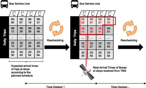
Figure 1 shows that at the beginning of the day we have a set of expected arrival times (EAT) for each bus trip at each bus stop that define the daily schedule. Note that the daily schedule is constructed by setting the dispatching times of each daily trip and estimating the arrival times of trips at stops by using travel time and dwell time information. The EATs of bus trips at stops are generally estimated with the use of historical automated vehicle location (AVL) data (Hounsell, Shrestha, & Wong, 2012; Shen, Xu, & Zeng, 2016). After some time period (Time Horizon 1), the bus positioning data generated by the in-vehicle telematics is processed to extract the actual arrival times (AAT) of the running trips at the stops. The obtained AATs provide new information to the bus rescheduling problem and are used together with the EATs of the remaining trips of the day to modify the dispatching times of the remaining trips.

This procedure is iterative and terminates at the end of the daily operations. For instance, there will be time horizons 2, 3,… where at each time horizon the generated AVL data is processed to extract the arrival times of bus trips at stops. Then, it is used as input, along with the EATs of the remaining daily trips, for rescheduling the operations of the remaining trips.

To model this rolling-horizon optimization problem, three 2-dimensional matrices A, E and D are introduced. The dimensions of these matrices are $\left|N\right|\times \left|S\right|$ where $\left|N\right|$ is the number of planned daily trips for one service line and $\left|S\right|$ the number of stops of that line. Each element $a_{i,j}$ of matrix A represents the AAT of bus trip i at bus stop j if this information is already available from AVL data. In case it is not, then a dummy value is used ($a_{i,j}$ is set equal to 0 to indicate that this trip has not arrived yet at stop j). In addition, each element $e_{i,j}$ of matrix E represents the EAT of bus trip i at bus stop j. Finally, matrix D is a combination of matrices A and E and is continuously updated at each rolling horizon instance. Matrix D comprises of the AATs of buses at bus stops and the EATs of future bus trips at the corresponding stops: (1) $$d_{i,j}=\{\begin{array}{cc}{a}_{i,j},\hfill & \text{if} a_{i,j}\ne 0\hfill \\ e_{i,j},\hfill & \text{otherwise}\hfill \end{array}$$(1)

Every time matrix A receives an update, the new information replaces the expected times of arrival at matrix D and a new optimization is performed considering matrix D as optimization input (re-scheduling in rolling horizons). The main notation used in the modeling phase is presented below.

Table

Sets/Lists
S= {1,2,…|S|}	the set of bus stops of one bus line
N= {1,2,…|N|}	the set of planned daily trips of one bus line
$Z_j$ (unitless)	a list that returns the previous trip $i\in N$ which was operated by the same bus as trip $j\in N.$ If trip j is the first trip for that bus, then $Z_j=0$
Parameters
$a_{i,j}$ (min)	the AAT of a bus trip $i\in N$ at stop $j\in S$ which is equal to zero if trip i has not arrived yet at stop j (future trip)
$r_{i,j}$ (min)	the scheduled arrival time of a bus trip i at stop j. These times are the times provided by the original schedule of the daily operations
$h_{i,j}$ (min)	the scheduled time headway (bumper to bumper) between bus trips i and i + 1 at the time of their arrival at stop j (note: $h_{i,j}=r_{i+1,j}-r_{i,j}$ and $i\in N\setminus \left\{\right|N\left|\right\}$)
$t_{i,j}$ (min)	the expected travel time of a bus trip i between stop j and j + 1 (note: $j\in S\setminus \left\{\right|S\left|\right\}$)
$l$ (min)	the minimum layover time in minutes between successive bus trips performed by the same bus
${\lambda }_{\rho ,j}$ (pass./min)	the passenger arrival rate at stop j during the ρ-th hour of the day expressed in passengers per minute
νj (%)	the expected percentage of onboard passengers that will alight at stop j. Note that ${\nu }_{\left|S\right|}$ is always equal to 100% because all onboard passengers will alight at the last stop, $\left|S\right|$
ψi (pass.)	the capacity of each bus trip $i\in N$ in number of passengers
δi (min)	the scheduled dispatching time of each bus trip $i\in N$ during the tactical planning phase
γj (min)	the scheduled average waiting time of passengers at stop $j\in S$
η1 (min/pass.)	required time for each additional passenger boarding
η2 (min/pass.)	required time for each additional passenger alighting
Decision variables
$x_i$ (min)	the dispatching deviation of each trip $i\in N$ from its scheduled dispatching time, δi. Each deviation xi belongs to an $\left|N\right|$-valued vector x that contains the dispatching time deviations of all daily trips and includes all our decision variables, where $x_i\in \mathbf{x}, \forall i\in N$
Variables
$e_{i,j}$(x) (min)	the EAT of a bus trip i at stop j
$d_{i,j}$(x) (min)	$d_{i,j}(\mathbf{x})=a_{i,j}$ if bus trip i has already arrived at bus stop j; otherwise, $d_{i,j}(\mathbf{x})=e_{i,j}(\mathbf{x})$
${\tilde{\gamma }}_j(\mathbf{x})$ (min)	the actual average waiting time of passengers at stop $j\in S$
$f$(x) (min)	the daily average excess waiting time of passengers at stops
${\beta }_{i,j}(\mathbf{x})$ (pass.)	the expected busload of trip i at stop j
$k_{i,j}(\mathbf{x})$ (min)	the expected dwell time of each bus trip $i\in N$ at each stop $j\in S$

The EAT of a bus trip i at stop j depends on the expected trip travel times between stops, the expected dwell times at stops, the scheduled dispatching time of the trip, δ_i, and the dispatching time modification during the rescheduling phase, x_i: (2) $$e_{i,j}(\mathbf{x})=({\delta }_i+x_i)+\sum _{\varphi =1}^{j-1}{t}_{i,\varphi }+\sum _{\varphi =1}^{j-1}{k}_{i,\varphi }(\mathbf{x})$$(2) where ${\sum }_{\varphi =1}^{j-1}{t}_{i,\varphi }$ is the sum of the expected link travel times from the dispatching stop until stop j and ${\sum }_{\varphi =1}^{j-1}{k}_{i,\varphi }(\mathbf{x})$ the sum of the dwell times.

2.1. Objective function

In high-frequency bus services, the main objective is the improvement of the service regularity by adhering to the scheduled headways. Transport authorities, such as the Transport for London (TfL), the Land Transport Authority (LTA) in Singapore and others measure the service regularity as the excessive time that passengers have to wait at stops. This EWT is the extra waiting time of passengers over and above the waiting time that might be expected if all the buses on the route run on time. It reflects the regularity of the service and is the difference between the actual average waiting time of passengers at bus stops and the scheduled average waiting time.

The average scheduled waiting time of passengers at a bus stop $j\in S$ is a fixed value which is obtained from the daily schedule of bus headways. Assuming random passenger arrivals at each stop $j\in S,$ the waiting time of the average passenger is equal to half the headway between two adjacent trips. Hence, the average scheduled waiting time is (Hounsell et al., 2012): (3) $${\gamma }_j=\frac{\sum _{i=1}^{\left|N\right|-1}{(r_{i+1,j}-r_{i,j})}^2}{2\sum _{i=1}^{\left|N\right|-1}(r_{i+1,j}-r_{i,j})}, \text{for} \text{each} \text{stop} j\in S$$(3)

Similarly, the actual average waiting time of passengers at a bus stop $j\in S$ is measured as $\frac{{\sum }_{i=1}^{\left|N\right|-1}{(a_{i+1,j}-a_{i,j})}^2}{2{\sum }_{i=1}^{\left|N\right|-1}(a_{i+1,j}-a_{i,j})}.$ During a rolling-horizon rescheduling instance, the AATs of several bus trips at the respected stops are not known yet. Therefore, the actual average waiting time of passengers at bus stops is replaced by a mixture of actual and expected waiting times: (4) $${\tilde{\gamma }}_j(\mathbf{x})=\frac{\sum _{i=1}^{\left|N\right|-1}{(d_{i+1,j}(\mathbf{x})-d_{i,j}(\mathbf{x}))}^2}{2\sum _{i=1}^{\left|N\right|-1}(d_{i+1,j}(\mathbf{x})-d_{i,j}(\mathbf{x}))}, \text{for} \text{each} \text{stop} j\in S$$(4) where $d_{i,j}(\mathbf{x})=a_{i,j}$ if bus trip i has already arrived at bus stop j and $d_{i,j}(\mathbf{x})=e_{i,j}(\mathbf{x})$ if not. The expected average excess waiting time (EWT) per passenger at a rolling horizon rescheduling instance is calculated then as follows (Transportation Research Group, 1997): (5) $$f(\mathbf{x})=\frac{1}{\sum _{j\in S}{\tilde{w}}_j}\sum _{j=1}^{\left|S\right|}{\tilde{w}}_j({\tilde{\gamma }}_j(\mathbf{x})-{\gamma }_j)$$(5) where ${\tilde{w}}_j\ge 0$ is a weight parameter for every stop $j\in S$ and is used to assign more weight to stops with higher passenger demand because schedule deviations at such stops will impact more the average waiting times of passengers. Note that in the extreme case where ${\tilde{w}}_j$ is set to zero for a stop $j\in S,$ that stop is not included in the consideration of schedule deviations (see Cats et al., 2011; Van Oort et al., 2010). Note also that the value of each weight parameter ${\tilde{w}}_j$ can be derived after calibration with the use of stop-level demand data from the actual operations.

In Equation (5)(5) $$f(\mathbf{x})=\frac{1}{\sum _{j\in S}{\tilde{w}}_j}\sum _{j=1}^{\left|S\right|}{\tilde{w}}_j({\tilde{\gamma }}_j(\mathbf{x})-{\gamma }_j)$$(5) , $f(\mathbf{x})$ is the objective function of the bus rescheduling problem at each rolling horizon optimization instance which should be minimized by computing new dispatching times that improve the service regularity.

2.2. Layover and capacity constraints

The layover time l consists of (i) the driver’s break time that is required before starting a next trip plus (ii) the required deadhead time for traveling from the last stop of the previous trip to the first stop of the next trip. The deadhead time might be equal to zero if the last stop of the previous trip and the first stop of the next one are the same.

To conform to the layover time constraint, the time difference between the starting time of trip i and the ending time of the previous trip Z_i should be greater than the layover time limit: (6) $$d_{i,1}(\mathbf{x})-\left(d_{Z_i,\left|S\right|}(\mathbf{x})+k_{i,\left|S\right|}(\mathbf{x})\right)\ge l, \forall i\in N$$(6)

Each trip $i\in N$ is also operated by a bus with a capacity ψ_i in number of passengers. Let ${\lambda }_{\rho ,j}$ be the passenger arrival rate at stop j during the ρ-th hour of the day expressed in passengers per minute. Note that the use of a different passenger arrival rate per hour ρ allows us to represent better the temporal demand variation across the day. Note also that the arrival rate ${\lambda }_{\rho ,j}$ does not depend on the arrival time of buses at the respective stops. This implies that passengers do not coordinate their arrival times at stops with the arrival times of buses. This assumption holds true for high-frequency services that are the focus of this study because if the headways are negligibly small, passengers do not consider the scheduled arrival times of buses when deciding about the timing of their arrival. In contrary, in low-frequency services passengers tend to consider the scheduled arrival times of buses and adjust the timing of their arrivals accordingly. Welding (1957) and Bartholdi and Eisenstein (2012) have established that passengers start to coordinate the timing of their arrivals at low-frequency services with less than five buses per hour.

Let also ν_j be the expected percentage of onboard passengers that will alight at stop j, where ${\nu }_{\left|S\right|}$ is always equal to 100% because all onboard passengers will alight at the last stop, $\left|S\right|.$ The busload ${\beta }_{i,j}(\mathbf{x})$ of bus trip $i\in \{2,3,\dots ,|N\left|\right\}$ when it departs from stop $j\in \{2,3,\dots ,|S\left|\right\}$ is expressed as: (7) $$\begin{array}{c}{\beta }_{i,j}(\mathbf{x})={\beta }_{i,j-1}(\mathbf{x})-{\nu }_j{\beta }_{i,j-1}(\mathbf{x})+{\lambda }_{\rho ,j}[\left(d_{i,j}(\mathbf{x})+k_{i,j}(\mathbf{x})\right)-\left(d_{i-1,j}(\mathbf{x})+k_{i-1,j}(\mathbf{x})\right)],\\ \forall i\in \{2,..,|N\left|\right\},j\in \{2,\dots ,|S\left|\right\}\end{array}$$(7)

Note that in Equation (7)(7) $$\begin{array}{c}{\beta }_{i,j}(\mathbf{x})={\beta }_{i,j-1}(\mathbf{x})-{\nu }_j{\beta }_{i,j-1}(\mathbf{x})+{\lambda }_{\rho ,j}[\left(d_{i,j}(\mathbf{x})+k_{i,j}(\mathbf{x})\right)-\left(d_{i-1,j}(\mathbf{x})+k_{i-1,j}(\mathbf{x})\right)],\\ \forall i\in \{2,..,|N\left|\right\},j\in \{2,\dots ,|S\left|\right\}\end{array}$$(7) the busload of a trip $i\in N\setminus \left\{1\right\}$ after it departs from stop $j\in S\setminus \left\{1\right\}$ is equal to its busload before arriving at stop j, expressed as ${\beta }_{i,j-1}(\mathbf{x}),$ minus the number of passengers that alighted at stop j, expressed as ${\nu }_j{\beta }_{i,j-1}(\mathbf{x}),$ plus the number of passengers boarding at stop j. The latter depends on the passenger arrival rate at stop j and the departure headway between trip i and its preceding one i–1 as it is expressed in the relation ${\lambda }_{\rho ,j}[(d_{i,j}(\mathbf{x})+k_{i,j}(\mathbf{x}))-(d_{i-1,j}(\mathbf{x})+k_{i-1,j}(\mathbf{x}))].$ Finally, we note that in Equation (7)(7) $$\begin{array}{c}{\beta }_{i,j}(\mathbf{x})={\beta }_{i,j-1}(\mathbf{x})-{\nu }_j{\beta }_{i,j-1}(\mathbf{x})+{\lambda }_{\rho ,j}[\left(d_{i,j}(\mathbf{x})+k_{i,j}(\mathbf{x})\right)-\left(d_{i-1,j}(\mathbf{x})+k_{i-1,j}(\mathbf{x})\right)],\\ \forall i\in \{2,..,|N\left|\right\},j\in \{2,\dots ,|S\left|\right\}\end{array}$$(7) , the expected percentage of onboard passengers that will alight at stop j is not time-dependent. This might not always be true in practice because the distribution of passenger demand might vary across time. In such case, and without loss of generality, v_j can be replaced by $v_{j,\omega },$ where ω is the time period within which the value of v_j remains stable.

Equation (7)(7) $$\begin{array}{c}{\beta }_{i,j}(\mathbf{x})={\beta }_{i,j-1}(\mathbf{x})-{\nu }_j{\beta }_{i,j-1}(\mathbf{x})+{\lambda }_{\rho ,j}[\left(d_{i,j}(\mathbf{x})+k_{i,j}(\mathbf{x})\right)-\left(d_{i-1,j}(\mathbf{x})+k_{i-1,j}(\mathbf{x})\right)],\\ \forall i\in \{2,..,|N\left|\right\},j\in \{2,\dots ,|S\left|\right\}\end{array}$$(7) cannot be applied for all trips i and stops j. Namely, we require boundary conditions for trip i = 1 and stop j = 1. In more detail, there is no trip preceding the first trip of the day, i = 1. Hence, for i = 1 the busload ${\beta }_{1,j}(\mathbf{x})$ is expressed as: (8) $${\beta }_{1,j}(\mathbf{x})={\beta }_{1,j-1}(\mathbf{x})-{\nu }_j{\beta }_{1,j-1}(\mathbf{x})+{\tilde{b}}_j, \forall j\in \{2,\dots ,|S\left|\right\}$$(8) where ${\tilde{b}}_j$ are the expected passenger boardings at each stop j for the first trip of the day.

The second boundary condition is related to the busload at the first stop. When a bus arrives at the first stop is initially empty. Additionally, there are no alightings at the first stop. That is, (9) $${\beta }_{i,1}(\mathbf{x})={\lambda }_{\rho ,1}[\left(d_{i,1}(\mathbf{x})+k_{i,1}(\mathbf{x})\right)-\left(d_{i-1,1}(\mathbf{x})+k_{i-1,1}(\mathbf{x})\right)],\forall i\in \{2,..,|N\left|\right\}$$(9) and (10) $${\beta }_{1,1}(\mathbf{x})={\tilde{b}}_1$$(10)

Obviously, in order to ensure that the busload is always below the capacity of the bus that operates trip i, the following inequality constraint should be satisfied at all bus stops: (11) $${\psi }_i\ge {\beta }_{i,j}(\mathbf{x}), i\in N,\forall j\in S$$(11) where ψ_i is the capacity of each bus trip $i\in N$ in number of passengers. The layover and capacity constraints result in a total of $\left|N\right|+\left|N\right|\left|S\right|$ linear inequality constraints for the bus rescheduling problem.

Additionally, assuming that

1. passengers use the same door channel for boardings and alightings

2. there are no additional passenger arrivals while the bus is dwelling since the dwell time is negligibly small

the dwell time of trip $i\in N\setminus \left\{1\right\}$ at stop $j\in S\setminus \left\{1\right\}$ is: (12) $$k_{i,j}(\mathbf{x})={\eta }_1{\lambda }_{\rho ,j}\left[d_{i,j}(\mathbf{x})-d_{i-1,j}(\mathbf{x})\right]+{\eta }_2{\nu }_j{\beta }_{i,j-1}(\mathbf{x})$$(12)

where ${\eta }_1{\lambda }_{\rho ,j}\left[d_{i,j}(\mathbf{x})-d_{i-1,j}(\mathbf{x})\right]$ is the required time for passenger boardings and ${\eta }_2{\nu }_j{\beta }_{i,j-1}(\mathbf{x})$ the required time for passenger alightings of trip i at stop j.

When buses depart from the first stop, we do not have passenger alightings. Hence, the following boundary condition applies: (13) $$k_{i,1}(\mathbf{x})={\eta }_1{\lambda }_{\rho ,1}\left[d_{i,1}(\mathbf{x})-d_{i-1,1}(\mathbf{x})\right]$$(13)

2.3. Mathematical program of the rescheduling problem

The dispatching time modifications, x, of bus trips can theoretical take any integer value. It is prudent though to ensure that the rescheduled dispatching times do not differ significantly from the originally planned ones because this can affect (a) the crew schedules; and (b) the practical implementation of the rescheduling. For this reason, we enforce any dispatching time modification x_i from its planned dispatching time δ_i to be within the range of ±30 minutes. Therefore, each decision variable can take any value from the discrete set $Q=\{-30,-29,\dots ,0,\dots ,+29,+30\}$ min.

At a rolling-horizon optimization instance, dispatching time modifications can only be applied to future trips that have not been dispatched yet. For past trips that have been already dispatched, the dispatching time modifications are set equal to zero. Note that if a bus trip i is already dispatched, this is indicated by $a_{i,j}\ne 0$ at stop j = 1. Therefore: (14) $$x_i=\{\begin{array}{c}\text{any} \text{value} \text{from} \text{the} \text{set} Q \text{if} a_{i,1}=0\hfill \\ 0 \text{otherwise}\hfill \end{array}$$(14)

To calculate the dispatching times of the remaining trips of the day that minimize the EWTs of passengers at a rolling-horizon optimization instance, the following Integer Nonlinear Programing (INL) problem needs to be solved in near real-time: (15) $$\begin{array}{c}\underset{{}_{\mathbf{x}}}{\min }f(\mathbf{x})=\frac{1}{\sum _{{\tilde{w}}_j}{\tilde{w}}_j}\sum _{j=1}^{\left|S\right|}{\tilde{w}}_j\left(\frac{\sum _{i=1}^{\left|N\right|-1}{(d_{i+1,j}(\mathbf{x})-d_{i,j}(\mathbf{x}))}^2}{2\sum _{i=1}^{\left|N\right|-1}(d_{i+1,j}(\mathbf{x})-d_{i,j}(\mathbf{x}))}-\frac{\sum _{i=1}^{\left|N\right|-1}{(r_{i+1,j}-r_{i,j})}^2}{2\sum _{i=1}^{\left|N\right|-1}(r_{i+1,j}-r_{i,j})}\right)\\ \mathrm{s}.\mathrm{t}. d_{i,1}(\mathbf{x})-\left(d_{Z_i,\left|S\right|}(\mathbf{x})+k_{i,\left|S\right|}(\mathbf{x})\right)-l\ge 0, \forall i\in N\\ {\psi }_i\ge {\beta }_{i,j}(\mathbf{x}), \forall j\in S,\forall i\in N\\ x_i=\{\begin{array}{c}{x}_i\in Q \text{if} a_{i,1}=0\hfill \\ x_i=0 \text{otherwise}\hfill \end{array}\\ {\beta }_{i,j}(\mathbf{x})={\beta }_{i,j-1}(\mathbf{x})-{\nu }_j{\beta }_{i,j-1}(\mathbf{x})+{\lambda }_{\rho ,j}[\left(d_{i,j}(\mathbf{x})+k_{i,j}(\mathbf{x})\right)-\left(d_{i-1,j}(\mathbf{x})+k_{i-1,j}(\mathbf{x})\right)],\\ \hspace{1em} \forall i\in N\setminus \left\{1\right\},j\in S\setminus \left\{1\right\} \text{where} d_{i,j}(\mathbf{x})\in \rho -\text{th} \text{hour}\\ {\beta }_{1,j}(\mathbf{x})={\beta }_{1,j-1}(\mathbf{x})-{\nu }_j{\beta }_{1,j-1}(\mathbf{x})+{\tilde{b}}_j, \forall j\in \{2,\dots ,|S\left|\right\}\\ {\beta }_{i,1}(\mathbf{x})={\lambda }_{\rho ,1}[\left(d_{i,1}(\mathbf{x})+k_{i,1}(\mathbf{x})\right)-\left(d_{i-1,1}(\mathbf{x})+k_{i-1,1}(\mathbf{x})\right)], \forall i\in N\setminus \left\{1\right\}\wedge d_{i,1}(\mathbf{x})\in \rho -\text{th} \text{hour}\\ {\beta }_{1,1}(\mathbf{x})={\tilde{b}}_1\\ d_{i,j}(\mathbf{x})=\{\begin{array}{cc}{a}_{i,j},\hfill & \text{if}{a}_{i,j}\ne 0\hfill \\ e_{i,j}(\mathbf{x}),\hfill & \text{otherwise}\hfill \end{array}\\ e_{i,j}(\mathbf{x})=({\delta }_i+x_i)+\sum _{\varphi =1}^{j-1}{t}_{i,\varphi }+\sum _{\varphi =1}^{j-1}{k}_{i,\varphi }(\mathbf{x})\\ k_{i,j}(\mathbf{x})={\eta }_1{\lambda }_{\rho ,j}\left[d_{i,j}(\mathbf{x})-d_{i-1,j}(\mathbf{x})\right]+{\eta }_2{\nu }_j{\beta }_{i,j-1}(\mathbf{x}),\forall i\in N\setminus \left\{1\right\},\forall j\in S\setminus \left\{1\right\}\\ k_{i,1}(\mathbf{x})={\eta }_1{\lambda }_{\rho ,1}\left[d_{i,1}(\mathbf{x})-d_{i-1,1}(\mathbf{x})\right],\forall i\in N\setminus \left\{1\right\}\\ Q=\{-30,-29,\dots ,0,\dots ,+29,+30\} \text{min}.\end{array}$$(15)

This combinatorial optimization problem has $\left|N\right|+\left|N\right|\left|S\right|$ linear constraints and a fractional, nonlinear objective function. Given its integer programing nature, the problem is NP-Hard and because of its fractional objective function its continuous relaxation cannot be solved to optimality with analytical methods. For this reason, a globally optimal solution can be computed only with exhaustive search of the solution space (brute force) which can only be applied to small-scale problems.

Lemma 2.1.

The size of the solution space increases exponentially with the number of bus trips that need be rescheduled.

Proof.

Let $n\subseteq N$ be the subset of daily trips that have not been dispatched at the time instance we perform a rescheduling. Given the combinatorial nature of the problem, the dispatching time modification of each trip $i\in n$ can take one of the $\left|Q\right|=61$ values from the set $Q=\{-30,\dots ,+30\}$ min. If the dispatching time modifications of all trips in the set n are fixed and one needs to find the optimal dispatching time modification of only one bus trip $i\in n,$ then $\left|Q\right|=61$ different options need to be explored. If one needs to determine the optimal dispatching times of all trips from the set n, then the number of combinations that need to be evaluated becomes $|Q{|}^{\left|n\right|}$ and the solution space exploration increases exponentially with the number of trips that need to be rescheduled.□

Since the size of the solution space increases exponentially with the number of trips that need to be rescheduled, only small-scale scenarios can be exhaustively explored because of the incurred computational cost (i.e., the solution space when rescheduling only eight trips contains ${61}^8=1.9E+14$ alternative combinations).

3. Rolling-horizon rescheduling with SHC

Instead of exploring exhaustively the solution space of the rescheduling problem at each rolling horizon optimization instance, we use a SHC meta-heuristic to obtain a (potentially good) rescheduling solution in near real-time by exploring only a targeted portion of the entire solution space.

In a first step, a direction for the solution search is provided by assigning a higher priority to the satisfaction of constraints. This is achieved by introducing a penalty function which approximates the constrained rescheduling optimization problem with an unconstrained one.

Penalty function methods started to gain attention in the late 1960s (Fiacco & McCormick, 1968). These methods add a term to the objective function that introduces a high cost when constraints are violated (Bertsekas, 1990). In this work, we use exterior point penalization; nevertheless, there are also several interior point penalization methods in literature with most notable the work of Karmarkar (1984) which introduces a barrier against leaving the feasible region.

In this study, we use exterior point penalization because interior penalty functions require to start the solution search from an initial solution guess that satisfies all constraints (feasible solution guess) and finding a feasible initial solution is not a trivial task for multi-variate optimization problems. When using an exterior point penalty function, each constraint penalizes the objective function by a positive value which increases progressively its penalization as described in the following unconstrained optimization problem of Equation (16)(16) $$\begin{array}{c}\underset{\mathbf{x}}{\text{argmin}}p(\mathbf{x})=f(\mathbf{x})+\sum _{i=1}^{\left|N\right|+\left|N\right|\left|S\right|}{W}_i{(\text{min}[0,c_i(\mathbf{x})])}^2\\ \mathrm{s}.\mathrm{t}. \hspace{0.17em}{x}_i=\{\begin{array}{c}{x}_i\in Q \text{if} a_{i,1}=0\hfill \\ x_i=0 \text{otherwise}\hfill \end{array}\\ {\beta }_{i,j}(\mathbf{x})={\beta }_{i,j-1}(\mathbf{x})-{\nu }_j{\beta }_{i,j-1}(\mathbf{x})+{\lambda }_{\rho ,j}[\left(d_{i,j}(\mathbf{x})+k_{i,j}(\mathbf{x})\right)-\left(d_{i-1,j}(\mathbf{x})+k_{i-1,j}(\mathbf{x})\right)],\\ \hspace{1em} \forall i\in N\setminus \left\{1\right\},j\in S\setminus \left\{1\right\} \text{where} d_{i,j}(\mathbf{x})\in \rho -\text{th} \text{hour}\\ {\beta }_{1,j}(\mathbf{x})={\beta }_{1,j-1}(\mathbf{x})-{\nu }_j{\beta }_{1,j-1}(\mathbf{x})+{\tilde{b}}_j, \forall j\in \{2,\dots ,|S\left|\right\}\\ {\beta }_{i,1}(\mathbf{x})={\lambda }_{\rho ,1}[\left(d_{i,1}(\mathbf{x})+k_{i,1}(\mathbf{x})\right)-\left(d_{i-1,1}(\mathbf{x})+k_{i-1,1}(\mathbf{x})\right)], \forall i\in N\setminus \left\{1\right\}\wedge d_{i,1}(\mathbf{x})\in \rho -\text{th} \text{hour}\\ {\beta }_{1,1}(\mathbf{x})={\tilde{b}}_1\\ d_{i,j}(\mathbf{x})=\{\begin{array}{cc}{a}_{i,j},\hfill & \text{if}{a}_{i,j}\ne 0\hfill \\ e_{i,j}(\mathbf{x}),\hfill & \text{otherwise}\hfill \end{array}\\ e_{i,j}(\mathbf{x})=({\delta }_i+x_i)+\sum _{\varphi =1}^{j-1}{t}_{i,\varphi }+\sum _{\varphi =1}^{j-1}{k}_{i,\varphi }(\mathbf{x})\\ k_{i,j}(\mathbf{x})={\eta }_1{\lambda }_{\rho ,j}\left[d_{i,j}(\mathbf{x})-d_{i-1,j}(\mathbf{x})\right]+{\eta }_2{\nu }_j{\beta }_{i,j-1}(\mathbf{x}),\forall i\in N\setminus \left\{1\right\},\forall j\in S\setminus \left\{1\right\}\\ k_{i,1}(\mathbf{x})={\eta }_1{\lambda }_{\rho ,1}\left[d_{i,1}(\mathbf{x})-d_{i-1,1}(\mathbf{x})\right],\forall i\in N\setminus \left\{1\right\}\\ Q=\{-30,-29,\dots ,0,\dots ,+29,+30\} \text{min}.\end{array}$$(16) that approximates the constrained one of Equation (15)(15) $$\begin{array}{c}\underset{{}_{\mathbf{x}}}{\min }f(\mathbf{x})=\frac{1}{\sum _{{\tilde{w}}_j}{\tilde{w}}_j}\sum _{j=1}^{\left|S\right|}{\tilde{w}}_j\left(\frac{\sum _{i=1}^{\left|N\right|-1}{(d_{i+1,j}(\mathbf{x})-d_{i,j}(\mathbf{x}))}^2}{2\sum _{i=1}^{\left|N\right|-1}(d_{i+1,j}(\mathbf{x})-d_{i,j}(\mathbf{x}))}-\frac{\sum _{i=1}^{\left|N\right|-1}{(r_{i+1,j}-r_{i,j})}^2}{2\sum _{i=1}^{\left|N\right|-1}(r_{i+1,j}-r_{i,j})}\right)\\ \mathrm{s}.\mathrm{t}. d_{i,1}(\mathbf{x})-\left(d_{Z_i,\left|S\right|}(\mathbf{x})+k_{i,\left|S\right|}(\mathbf{x})\right)-l\ge 0, \forall i\in N\\ {\psi }_i\ge {\beta }_{i,j}(\mathbf{x}), \forall j\in S,\forall i\in N\\ x_i=\{\begin{array}{c}{x}_i\in Q \text{if} a_{i,1}=0\hfill \\ x_i=0 \text{otherwise}\hfill \end{array}\\ {\beta }_{i,j}(\mathbf{x})={\beta }_{i,j-1}(\mathbf{x})-{\nu }_j{\beta }_{i,j-1}(\mathbf{x})+{\lambda }_{\rho ,j}[\left(d_{i,j}(\mathbf{x})+k_{i,j}(\mathbf{x})\right)-\left(d_{i-1,j}(\mathbf{x})+k_{i-1,j}(\mathbf{x})\right)],\\ \hspace{1em} \forall i\in N\setminus \left\{1\right\},j\in S\setminus \left\{1\right\} \text{where} d_{i,j}(\mathbf{x})\in \rho -\text{th} \text{hour}\\ {\beta }_{1,j}(\mathbf{x})={\beta }_{1,j-1}(\mathbf{x})-{\nu }_j{\beta }_{1,j-1}(\mathbf{x})+{\tilde{b}}_j, \forall j\in \{2,\dots ,|S\left|\right\}\\ {\beta }_{i,1}(\mathbf{x})={\lambda }_{\rho ,1}[\left(d_{i,1}(\mathbf{x})+k_{i,1}(\mathbf{x})\right)-\left(d_{i-1,1}(\mathbf{x})+k_{i-1,1}(\mathbf{x})\right)], \forall i\in N\setminus \left\{1\right\}\wedge d_{i,1}(\mathbf{x})\in \rho -\text{th} \text{hour}\\ {\beta }_{1,1}(\mathbf{x})={\tilde{b}}_1\\ d_{i,j}(\mathbf{x})=\{\begin{array}{cc}{a}_{i,j},\hfill & \text{if}{a}_{i,j}\ne 0\hfill \\ e_{i,j}(\mathbf{x}),\hfill & \text{otherwise}\hfill \end{array}\\ e_{i,j}(\mathbf{x})=({\delta }_i+x_i)+\sum _{\varphi =1}^{j-1}{t}_{i,\varphi }+\sum _{\varphi =1}^{j-1}{k}_{i,\varphi }(\mathbf{x})\\ k_{i,j}(\mathbf{x})={\eta }_1{\lambda }_{\rho ,j}\left[d_{i,j}(\mathbf{x})-d_{i-1,j}(\mathbf{x})\right]+{\eta }_2{\nu }_j{\beta }_{i,j-1}(\mathbf{x}),\forall i\in N\setminus \left\{1\right\},\forall j\in S\setminus \left\{1\right\}\\ k_{i,1}(\mathbf{x})={\eta }_1{\lambda }_{\rho ,1}\left[d_{i,1}(\mathbf{x})-d_{i-1,1}(\mathbf{x})\right],\forall i\in N\setminus \left\{1\right\}\\ Q=\{-30,-29,\dots ,0,\dots ,+29,+30\} \text{min}.\end{array}$$(15) . (16) $$\begin{array}{c}\underset{\mathbf{x}}{\text{argmin}}p(\mathbf{x})=f(\mathbf{x})+\sum _{i=1}^{\left|N\right|+\left|N\right|\left|S\right|}{W}_i{(\text{min}[0,c_i(\mathbf{x})])}^2\\ \mathrm{s}.\mathrm{t}. \hspace{0.17em}{x}_i=\{\begin{array}{c}{x}_i\in Q \text{if} a_{i,1}=0\hfill \\ x_i=0 \text{otherwise}\hfill \end{array}\\ {\beta }_{i,j}(\mathbf{x})={\beta }_{i,j-1}(\mathbf{x})-{\nu }_j{\beta }_{i,j-1}(\mathbf{x})+{\lambda }_{\rho ,j}[\left(d_{i,j}(\mathbf{x})+k_{i,j}(\mathbf{x})\right)-\left(d_{i-1,j}(\mathbf{x})+k_{i-1,j}(\mathbf{x})\right)],\\ \hspace{1em} \forall i\in N\setminus \left\{1\right\},j\in S\setminus \left\{1\right\} \text{where} d_{i,j}(\mathbf{x})\in \rho -\text{th} \text{hour}\\ {\beta }_{1,j}(\mathbf{x})={\beta }_{1,j-1}(\mathbf{x})-{\nu }_j{\beta }_{1,j-1}(\mathbf{x})+{\tilde{b}}_j, \forall j\in \{2,\dots ,|S\left|\right\}\\ {\beta }_{i,1}(\mathbf{x})={\lambda }_{\rho ,1}[\left(d_{i,1}(\mathbf{x})+k_{i,1}(\mathbf{x})\right)-\left(d_{i-1,1}(\mathbf{x})+k_{i-1,1}(\mathbf{x})\right)], \forall i\in N\setminus \left\{1\right\}\wedge d_{i,1}(\mathbf{x})\in \rho -\text{th} \text{hour}\\ {\beta }_{1,1}(\mathbf{x})={\tilde{b}}_1\\ d_{i,j}(\mathbf{x})=\{\begin{array}{cc}{a}_{i,j},\hfill & \text{if}{a}_{i,j}\ne 0\hfill \\ e_{i,j}(\mathbf{x}),\hfill & \text{otherwise}\hfill \end{array}\\ e_{i,j}(\mathbf{x})=({\delta }_i+x_i)+\sum _{\varphi =1}^{j-1}{t}_{i,\varphi }+\sum _{\varphi =1}^{j-1}{k}_{i,\varphi }(\mathbf{x})\\ k_{i,j}(\mathbf{x})={\eta }_1{\lambda }_{\rho ,j}\left[d_{i,j}(\mathbf{x})-d_{i-1,j}(\mathbf{x})\right]+{\eta }_2{\nu }_j{\beta }_{i,j-1}(\mathbf{x}),\forall i\in N\setminus \left\{1\right\},\forall j\in S\setminus \left\{1\right\}\\ k_{i,1}(\mathbf{x})={\eta }_1{\lambda }_{\rho ,1}\left[d_{i,1}(\mathbf{x})-d_{i-1,1}(\mathbf{x})\right],\forall i\in N\setminus \left\{1\right\}\\ Q=\{-30,-29,\dots ,0,\dots ,+29,+30\} \text{min}.\end{array}$$(16)

where $c_i(\mathbf{x}), \forall i\in \{1,\dots ,|N|+|N\left|\right|S\left|\right\}$ are the inequality constraints related to the layover times and the vehicle capacities. In the penalty function $p(\mathbf{x}),$ the terms $W_i\gg 0$ are positive numbers and have sufficiently high values for ensuring that the satisfaction of the layover and the vehicle capacity constraints has a higher priority than the reduction of the excessive passenger waiting times.

The penalty function, $p(\mathbf{x}),$ is formulated in such way that:

• is equal to the objective function value, $f(\mathbf{x}),$ if all constraints are satisfied (the penalty function value of a feasible solution is equal to its objective function);

• does not penalize constraints that are satisfied. I.e., if for a solution x one constraint $c_i(\mathbf{x})$ is not violated, then $c_i(\mathbf{x})\ge 0$ and, as a result, min$[0,c_i(\mathbf{x})]=0;$

• penalizes progressively the violation of constraints since the violation of a constraint $c_i(\mathbf{x})<0$ is squared: $W_i{(\text{min}[0,c_i(\mathbf{x})])}^2)=W_i{c}_i^2(\mathbf{x}).$

In the SHC search, the dispatching time modifications of the bus trips that are not dispatched yet are initialized as $x_i=0, \forall i\in n\subseteq N.$ After that, the initial solution x is evaluated by calculating the penalty function value $p(\mathbf{x}).$ Hill climbing attempts to minimize the target function $p(\mathbf{x})$ by adjusting a single element of x at each step and determining whether the change improves the penalty function score. This differs from gradient descent methods, which adjust all the values in x at each step according to the gradient of the hill. Note that in our case we cannot apply gradient descent methods because our problem is not continuous and the function $p(\mathbf{x})$ is not differentiable at every point of its domain due to its $\text{min}[0,c_i(\mathbf{x})]{)}^2$ terms.

The proposed SHC search comprises of the following stages:

• an initial trip, ι, is randomly selected from the set n;

• for this trip, we change the value of $x_{\iota }$ by selecting a value from the set Q. If the selected value reduces the penalty function score this value is adopted; otherwise is discarded. This procedure continues until exploring all the values from set Q;

• the previous procedure is performed for all other trips $i\in n\setminus \left\{\iota \right\}$ in a sequential order;

• another trip $\iota \in n$ is randomly selected and the above-described procedure is repeated until reaching the maximum number of allowed iterations, μ^max.

This procedure can be translated into the following algorithm:

Algorithm 1

1: function Sequential Hill Climbing

2:  Initialize $x_i=0, \forall i\in n;$

3:  while μ^max is not reached do

4:   Select randomly an initial trip $\iota \in n;$

5:   for each $q\in Q$ do

6:    Set $u\leftarrow x_{\iota };$

7:    Set $x_{\iota }\leftarrow q;$

8:    if $p(\mathbf{x})$ is not improved by this change then

9:     Set $x_{\iota }$ back to its previous value: $x_{\iota }\leftarrow u;$

10:    end if

11:   end for

12:   for each $i\in n\setminus \left\{\iota \right\}$ do

13:    for each $q\in Q$ do

14:     Set $u\leftarrow x_i;$

15:     Set $x_i\leftarrow q;$

16:     if $p(\mathbf{x})$ is not improved by this change then

17:      Set x_i back to its previous value: $x_i\leftarrow u;$

18:     end if

19:    end for

20:   end for

21:  end while

22:  return optimal solution x of the dispatching time modifications;

23: end function

The hill-climbing search is sequential because the algorithm does not optimize the dispatching times of all remaining trips in one step. Instead, the algorithm starts from one randomly selected trip and searches the dispatching time modification that reduces the penalty function score the most. Then, this procedure is performed for all other trips in a sequential order, where at each sequence only the dispatching time modifications of the examined trip are explored. In the proposed algorithm, at each iteration another trip is randomly selected for performing a SHC search in a multi-start manner (this random-restart hill climbing search is also known as Shotgun hill climbing and is effective because it spends resources on exploring the solution space, rather than carefully optimizing the initial solution Deb, 2001).

Lemma 3.1.

The number of computations of the sequential hill climbing search increases polynomially with the number of allowed iterations, μ^max, and the number of remaining trips, n, that need to be rescheduled.

Proof.

In the algorithmic description of the sequential hill climbing algorithm, each random-restart hill-climbing iteration contains two nested for loops that perform a fixed number of $\left|n\right|·\left|Q\right|$ calculations. With these calculations, the dispatching time modifications that improved the performance of each trip are computed in a sequential order. Then, the same operation is performed μ^max times by restarting the sequential search from another randomly selected trip; thus, requiring a total amount of $\left|n\right|\left|Q\right|{\mu }^{\text{max}}$ computations that increase polynomially with the size of the remaining trips, n, and the number of allowed iterations, μ^max.

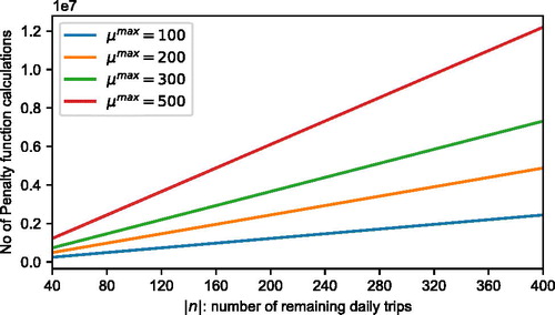
The opportunistic exploration of the combinatorial solution space with the random-restart sequential hill climbing (SHC) search is scalable due to its polynomial complexity and can find an improved solution to the bus rescheduling problem in near real-time even for high-frequency bus lines with multiple stops. In Figure 2, we present the computational requirements of the SHC search for rolling horizon rescheduling instances with different numbers of remaining trips and different optimization termination, μ^max, thresholds. Note that a maximum number of 400 remaining trips is adopted because, in general, a high-frequency bus line with a frequency of 20 trips/h is not expected to operate more than 400 trips during the daily operational hours.

Figure 2. Required number of penalty function evaluations for different numbers of remaining trips to be rescheduled with sequential hill climbing.

In the next section, the effect of rolling horizon rescheduling to the regularity of the daily bus operations is tested using GTFS-realtime data from bus line 15 L in Denver, USA.

4. Numerical experiments

4.1. Case study description

In the case study, we use GTFS-RT data from bus line 15 L in Denver, USA to (i) measure how much the actual EWTs of passengers differ from the planned ones; and (ii) compute the potential gain in service regularity if the dispatching times of buses are periodically rescheduled.

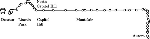
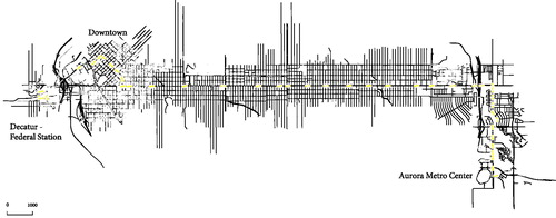
Bus line 15 L (Figure 3) is a bus line with 42 bus stops that connects the east part of the Denver metropolitan area with a main train station at the south west (Aurora Metro Center). This is a high-frequency line and serves the downtown area of the city. The first trip of the day is planned at 6:02 am and the last trip of the day is expected to arrive at the terminal around 1:03 am (for the planned arrival times at selected stops, the interested reader can refer to: http://www3.rtd-denver.com/schedules/getSchedule.action?routeId=15L). As a high-frequency service, we assume that passengers do not coordinate the timing of their arrivals with the arrival times of buses at stops (Bartholdi & Eisenstein, 2012; Welding, 1957). Despite this assumption, we note that the transport authority in Denver offers real-time information about the positions of buses and updates their arrival time predictions at least every 30 s. Consequently, passengers that have access to real-time information on their mobile phones might want to coordinate their arrival times at stops to the EATs of buses even in this high frequency line.

Figure 3. Topology of the 42 bus stops of bus line 15 L.

Starting from the beginning of the day (6 am), the GTFS-RT data from the running vehicles is processed in time intervals of 15 min. The newly generated GTFS-RT data during each time interval is used to update the AATs of buses at stops. It also updates the matrix D that combined the actual and EATs of bus trips at stops. The updated matrix D is used for re-computing new dispatching times for the remaining trips of the day at each rolling horizon (i.e. end of the 15-min interval). Thus, the total number of rolling horizon rescheduling instances from the beginning until the end of the day (6:02 am–1:03 am) is 78 and the initial daily schedule of bus line 15 L is updated 78 times.

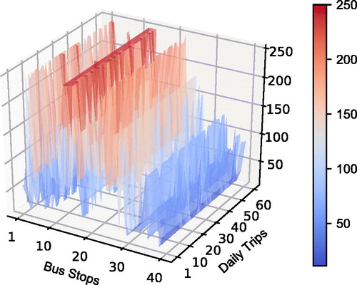
After analyzing the GTFS-RT data, one of the findings was that during the weekdays many planned bus trips are canceled. For this reason, we selected Saturday for the numerical experiments because we observed that on Saturdays almost all planned trips are operated without cancelations. This allows us to have a less biased comparison between the scheduled waiting times of passengers and the actual ones. On Saturdays, the scheduled number of operational trips from 6:02 am to 1:03am is 61. To calculate the EATs of future bus trips to stops, we processed 4 months of historical AVL data from Saturday operations and estimated the travel times of trips between consecutive bus stops (Figure 4).

Figure 4. Average Travel Times between consecutive stops in seconds for each one of the 61 Saturday trips.

From the 42 bus stops of the examined bus line, only a subset of the 16 most significant bus stops is considered for the calculation of the passengers’ EWTs from the bus operator (namely, the stops 1, 4, 5, 8, 9, 12, 14, 15, 16, 19, 20, 24, 26, 29, 36, and 42). Consequently, we set ${\tilde{w}}_j=1$ for the 16 bus stops of the above set and ${\tilde{w}}_j=0$ for all other stops. Those 16 bus stops are the “control points” of the operations and are selected because they are either intersection stops or have high passenger boarding numbers, thus it is important to maintain a high level of regularity.

Initially, we use the GTFS-RT data from Saturday, July 22, 2017 to compare the AATs of bus trips at the 16 control point stops against the scheduled ones and derive the average EWT per passenger. On that day operated 60 trips out of the 61. The results of calculating the average EWT per passenger are summarized in Table 1. Note that the reported average daily passenger EWT (1.947 min) is calculated according to Equation (5)(5) $$f(\mathbf{x})=\frac{1}{\sum _{j\in S}{\tilde{w}}_j}\sum _{j=1}^{\left|S\right|}{\tilde{w}}_j({\tilde{\gamma }}_j(\mathbf{x})-{\gamma }_j)$$(5) and is the KPI of the service regularity. Note also that plugging in the values of ${\tilde{w}}_j$ in Equation (5)(5) $$f(\mathbf{x})=\frac{1}{\sum _{j\in S}{\tilde{w}}_j}\sum _{j=1}^{\left|S\right|}{\tilde{w}}_j({\tilde{\gamma }}_j(\mathbf{x})-{\gamma }_j)$$(5) we get $\frac{1}{\sum _{j\in S}{w}_j}=1/16.$

Table 1. Performance of the daily operations of bus line 15 L (Saturday, July 22nd, 2017).

Bus stop	Average passenger	Scheduled passenger	Bus stop	Average passenger	Scheduled passenger
	waiting time (min)	waiting time (min)		waiting time (min)	waiting time (min)
1	$\simeq 12.66$	10.61	16	$\simeq 12.87$	10.67
4	$\simeq 12.13$	10.61	19	$\simeq 12.80$	10.67
5	$\simeq 11.86$	10.61	20	$\simeq 12.79$	10.67
8	$\simeq 11.91$	10.62	24	$\simeq 12.83$	10.66
9	$\simeq 12.01$	10.62	26	$\simeq 12.86$	10.66
12	$\simeq 12.72$	10.63	29	$\simeq 12.90$	10.66
14	$\simeq 12.74$	10.65	36	$\simeq 12.85$	10.68
15	$\simeq 12.74$	10.66	42	$\simeq 12.78$	10.67
Daily passenger Excess Waiting Time: 1.947 min

This significant difference between the actual and the scheduled passenger waiting times occurred mainly because the (i) traffic conditions change during the day leading to significant differences between the expected and the actual trip travel times as concluded also from many works in the literature (Chang et al., 2010; Gurmu & Fan, 2014; Yan, Liu, Meng, & Jiang, 2013) and the (ii) dwell times of bus trips which are behind schedule increase creating a domino effect that leads to bus bunching.

For this reason, it is important to reschedule the dispatching times of the remaining daily trips periodically, as it is demonstrated in Subsection 4.4.

4.2. Computational tests and solution quality

In this subsection, we study the performance of the proposed SHC algorithm in terms of convergence (optimality gap) and computational costs when rescheduling the trips in our previously described case study.

With respect to the optimality gap tests, the solution of the SHC should be compared against a globally optimal solution. Our rolling-horizon rescheduling problem is NP-Hard, therefore a globally optimal solution can be computed only at small-scale problem instances. For this reason, the optimality gap of the SHC method is studied at small-scale scenarios that permit the computation of a globally optimal solution with brute force.

Regarding the computational cost tests, we compare the computational time of our algorithm against another common solution method for combinatorial optimization: the genetic algorithm. Even though both SHC and the genetic algorithm cannot guarantee the convergence to a globally optimal solution, their solution performance can be compared in larger-scale scenarios providing an indication of the effectiveness of our approach.

The results of the computational tests are summarized in Table 2. For a detailed explanation of the genetic algorithm used in these tests, the interested reader can refer to the Appendix. Note that all tests are conducted in a 2.40 GHz, quad-core processor with a 16GB RAM. The SHC algorithm is programed in Python 2.7 and the genetic algorithm is implemented with the use of the Distributed Evolutionary Algorithms in Python (Deap) package Fortin et al. (2012) in Python 2.7. Note that the hyperparameters of the genetic algorithm (namely, the population size, the mutation rate and the maximum population generations) have been calibrated for each scenario to guarantee that it will attain its best performance when compared against the SHC approach. Finally, the brute force approach is also programed in Python 2.7. and evaluates the performance of the objective function for each possible combination of rescheduled departure times.

Table 2. Performance of different solution methods in idealized scenarios.

Scenarios		Computational time			Optimized $p(\mathbf{x})$ score (sec)
No. of trips	No. of bus stops	Brute force	Sequential hill climbing	Genetic algorithm	Brute force	Sequential hill climbing	Genetic algorithm
2	20	3.83 sec	0.22 s	1.38 s	62.62	62.62	62.62
3	20	8 min	0.35 s	2.01 s	58.98	58.98	58.98
4	20	8 h 12 min	0.72 s	3.33 s	58.41	58.41	58.41
10	20	—	3.12 s	5.48 s	—	54.24	56.55
20	20	—	6.78 s	21.24 s	—	40.06	56.31
30	20	—	16.00 s	49.73 s	—	35.87	56.11
40	20	—	27.64 s	101.25 s	—	26.64	47.02
50	20	—	44.42 s	246.53 s	—	9.20	32.77
60	20	—	62.98 s	284.32 s	—	6.37	17.98

To perform the computational and solution quality tests, we reschedule the scenarios in Table 2 (ranging from 2 to 60 trips). Note that if we reschedule 2 trips, those are the last 2 of the day, if we reschedule 3 those are the last 3 and so forth. The upper rescheduling limit is 60 trips that contains the entirety of daily trips of our case study. For each scenario, we report the computational time of the brute force method, the SHC and the genetic algorithm. With the use of brute force, we can solve up to scenarios with four bus trips with a computational time of 8 h and 12 min. That is, the globally optimal solution can be established when rescheduling up to four trips. In addition, in the last three columns of Table 2 we report the optimized value of the objective function, $p(\mathbf{x})$ presented in Equation (16)(16) $$\begin{array}{c}\underset{\mathbf{x}}{\text{argmin}}p(\mathbf{x})=f(\mathbf{x})+\sum _{i=1}^{\left|N\right|+\left|N\right|\left|S\right|}{W}_i{(\text{min}[0,c_i(\mathbf{x})])}^2\\ \mathrm{s}.\mathrm{t}. \hspace{0.17em}{x}_i=\{\begin{array}{c}{x}_i\in Q \text{if} a_{i,1}=0\hfill \\ x_i=0 \text{otherwise}\hfill \end{array}\\ {\beta }_{i,j}(\mathbf{x})={\beta }_{i,j-1}(\mathbf{x})-{\nu }_j{\beta }_{i,j-1}(\mathbf{x})+{\lambda }_{\rho ,j}[\left(d_{i,j}(\mathbf{x})+k_{i,j}(\mathbf{x})\right)-\left(d_{i-1,j}(\mathbf{x})+k_{i-1,j}(\mathbf{x})\right)],\\ \hspace{1em} \forall i\in N\setminus \left\{1\right\},j\in S\setminus \left\{1\right\} \text{where} d_{i,j}(\mathbf{x})\in \rho -\text{th} \text{hour}\\ {\beta }_{1,j}(\mathbf{x})={\beta }_{1,j-1}(\mathbf{x})-{\nu }_j{\beta }_{1,j-1}(\mathbf{x})+{\tilde{b}}_j, \forall j\in \{2,\dots ,|S\left|\right\}\\ {\beta }_{i,1}(\mathbf{x})={\lambda }_{\rho ,1}[\left(d_{i,1}(\mathbf{x})+k_{i,1}(\mathbf{x})\right)-\left(d_{i-1,1}(\mathbf{x})+k_{i-1,1}(\mathbf{x})\right)], \forall i\in N\setminus \left\{1\right\}\wedge d_{i,1}(\mathbf{x})\in \rho -\text{th} \text{hour}\\ {\beta }_{1,1}(\mathbf{x})={\tilde{b}}_1\\ d_{i,j}(\mathbf{x})=\{\begin{array}{cc}{a}_{i,j},\hfill & \text{if}{a}_{i,j}\ne 0\hfill \\ e_{i,j}(\mathbf{x}),\hfill & \text{otherwise}\hfill \end{array}\\ e_{i,j}(\mathbf{x})=({\delta }_i+x_i)+\sum _{\varphi =1}^{j-1}{t}_{i,\varphi }+\sum _{\varphi =1}^{j-1}{k}_{i,\varphi }(\mathbf{x})\\ k_{i,j}(\mathbf{x})={\eta }_1{\lambda }_{\rho ,j}\left[d_{i,j}(\mathbf{x})-d_{i-1,j}(\mathbf{x})\right]+{\eta }_2{\nu }_j{\beta }_{i,j-1}(\mathbf{x}),\forall i\in N\setminus \left\{1\right\},\forall j\in S\setminus \left\{1\right\}\\ k_{i,1}(\mathbf{x})={\eta }_1{\lambda }_{\rho ,1}\left[d_{i,1}(\mathbf{x})-d_{i-1,1}(\mathbf{x})\right],\forall i\in N\setminus \left\{1\right\}\\ Q=\{-30,-29,\dots ,0,\dots ,+29,+30\} \text{min}.\end{array}$$(16) .

From Table 2, one can note that the optimized objective function value with the SHC approach is equal to that one with the brute force approach for scenarios with up to four bus trips. That is, SHC converges to a globally optimal solution and there is no optimality gap. For more than four trips, that point cannot be proved with absolute certainty due to the absence of a reliable benchmark. In scenarios with a higher number of trips, we note that SHC performs better than the genetic algorithm when rescheduling 20 trips or more. Particularly, in the rescheduling case of 60 trips, SHC results in an improved solution by 65% compared to the genetic algorithm. As it is presented in Figure 5, the main reason is that the population of the genetic algorithm is not improving any further after the 30th population generation. In contrast, SHC exhibits a rapid convergence and terminates with a $p(\mathbf{x})$ score of 6.37 s after only six iterations.

Figure 5. Convergence of the sequential hill climbing and the genetic algorithm when rescheduling 60 trips of bus line 15 L.

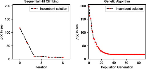
In terms of computational costs, SHC can reschedule 60 trips (which can be the entirety of the daily trips) in $\approx$1 minute using a conventional computing machine. This proves that we can reschedule a real-sized bus line in near real-time. Additionally, the SHC is consistently at least two times faster than the genetic algorithm. All in all, both approaches have a similar performance when rescheduling up to 20 trips. After that limit, SHC performs better both in terms of convergence and computational costs.

4.3. Sensitivity analysis of the EWT with respect to the range of dispatching time modifications, Q

In our case study, we allow the dispatching time modifications, x, to receive values from the set $Q=\{-30,-29,\dots ,0,\dots ,+29,+30\}$ min at each rescheduling optimization instance. Nevertheless, bus operators might not be willing to modify the dispatching times that much from their scheduled values, even if this is beneficial for the service regularity.

To investigate the influence of a restricted range of dispatching time modification options, we perform again the experiments of the previous section. We reschedule all 60 trips in Table 2 with the use of SHC and we alter every time the range of the dispatching time modification options, Q. The results are summarized in Table 3. The ranges tested in our evaluation are reported at the first column of Table 3. For each range of dispatching time modification options, we compute the optimized value of our objective function which is reported at the second column of the table.

Table 3. Sensitivity of solution performance to restrictions on dispatching time modifications, Q.

Range of Q	Optimized $p(\mathbf{x})$ score (sec)
$[-30$ min, + 30 min]	6.37 s
$[-25$ min, + 25 min]	6.58 s
$[-20$ min, + 20 min]	7.30 s
$[-15$ min, + 15 min]	8.03 s
$[-10$ min, + 10 min]	8.21 s
$[-7$ min, + 7 min]	17.03 s
$[-5$ min, + 5 min]	34.54 s
$[-4$ min, + 4 min]	38.86 s
$[-3$ min, + 3 min]	51.71 s
$[-2$ min, + 2 min]	68.03 s

Interestingly, the solution quality does not deteriorate immediately when we restrict the range of dispatching time modification options. Indeed, the solution quality remains relatively stable if we are allowed to modify the planned dispatching time of each trip by ±10 min. This can be easily noticed in Figure 6 that plots the results from Table 3. This finding suggests that we can attain significant improvements without disrupting completely the vehicle and crew schedules.

Figure 6. Solution sensitivity to different dispatching time modification restrictions, Q, when rescheduling all 60 trips of bus line 15 L.

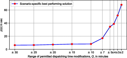
Contrary to the above, if we are only allowed to modify the dispatching times of trips by less than 10 min, then the potential benefit follows a sharp reduction. For modifications in the range of ±5 min, the potential gain shrinks resulting in an EWT of 38.86 s. This sharp deterioration of the solution quality continues and escalates for modification ranges of ±2 min. Consequently, a potential recommendation is to permit, when possible, dispatching time modifications in the range of 10 min.

4.4. Application of the periodic rescheduling

Splitting the operating time of the day into 15-min periods, we have 78 rolling horizons. At each rolling horizon instance, the dispatching times of the remaining daily trips are re-computed based on the new information regarding the AATs of buses at stops (GTFS-RT data). At each rolling-horizon instance, the observed arrival times of buses at stops are used together with the EATs of the remaining trips of the day for forming the matrix D and updating the dispatching times.

As the rolling horizons increase ($\to 78$) the rescheduling affects the dispatching times of a smaller fraction of trips because:

• several trips have already been dispatched; hence their dispatching time cannot be rescheduled.

• after several periodic optimizations, the degrees of freedom (i.e. rescheduling options) are limited and the operations cannot be improved further.

The rescheduling options at each rolling horizon are computed with the aim of minimizing the daily average EWT of passengers. Note that at a rolling horizon instance the average daily EWT of passengers comprises of the actual EWT (for trips that have already served the bus stops) and the expected EWT (for future trips for which we estimate their arrival times at stops). Hence, the daily average EWT evolves at every rolling horizon instance and stabilizes at the end of the day (rolling horizon 78) where all trips have completed their services and the value of the daily average EWT of passengers is definitive. The evolution of the daily average EWT at each periodic optimization instance is presented in Figure 7.

Figure 7. Projected value of the daily average excess waiting time of passengers at each periodic optimization instance. At the end of the day, the actual value after the 79 reschedulings becomes 0.92 min.

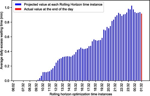
At the beginning of the day, the expected daily average EWT is close to zero. This means that the rescheduling will lead to high regularity levels if the AATs of future trips at stops are identical to the expected ones (something that is not the case in practice). However, this expectation changes after $\sim 15$ rolling horizons (at 9:47am) because the observed arrival times of buses differ considerably from the expected ones and the bus operations should adjust accordingly. Another important observation is that the expected daily average EWT at 00:02 exhibits a higher value than the observed one at the end of the day. This might occur in some occasions if the actual travel times of the remaining trips are more favorable than the expected ones leading to more even time headway distributions for the remaining trips.

5. Discussion and sensitivity analysis of performance under travel time noise

The observed EWT of passengers on Saturday, July 22nd was 1.947 min (cf. Table 1). With the use of periodic rescheduling on time intervals of 15 min, the daily EWT was reduced to 0.92 min (cf. Figure 7). This regularity improvement of $\simeq 50\%$ refers to that particular day. An interesting topic for further investigation though is the importance of the periodic rescheduling for different levels of travel time noise.

This is further examined by replicating the arrival times of buses at stops at the Simulator of Urban MObility (SUMO). To this end, we import the road network of Denver in SUMO using OpenStreetMaps. Then, we add the stop locations of bus line 15 L (see Figure 8). To replicate the arrival times of buses at stops, we calibrate the traffic flow-related parameters with the use of the Constrained Optimization BY Linear Approximation (COBYLA) algorithm from the SciPy library in Python.

Figure 8. Bus line 15 L in SUMO. To improve visibility, bus stops are enlarged and marked in yellow. Additionally, sidewalks and secondary streets have been removed.

COBYLA is a standard optimization algorithm which is used in SUMO to find the optimal parameter values of traffic flows and traffic signal cycles by minimizing the root mean square error (RMSE) between the observed and simulated arrival times of buses at stops (a well-known benchmark calibration with COBYLA is in Smilowitz, Daganzo, Cassidy, & Bertini, 1999). COBYLA terminates when an acceptable RMSE error is achieved indicating that the calibrated traffic scenario results in simulated arrival times at stops which are too close to the observed ones from the GTFS-RT data.

Apart from the traffic-related parameters, the vehicle parameters of the running buses (i.e., acceleration, max. speed, deceleration) are communicated to SUMO using a standard.xml file that follows the SUMO guidelines. Based on historical data from bus line 15 L, their values are set as follows: acceleration—2.61 m/s², deceleration—4.68 m/s², max. speed—62 miles/h. The RMSE error of our best performing traffic-related parameter values was 4.2%.

By using a traffic simulator, we investigate the performance of the periodic rescheduling in different scenarios considering the effect of travel time noise. The examined scenarios are summarized in Table 4. Each travel time noise scenario assumes that the actual link travel times follow a normal distribution where the mean value of each normal distribution is equal to the respective value of the expected link travel time.

Table 4. Characteristic of the normal distribution from which the actual link travel times are sampled for each trip $i\in N$ and link that connects the consecutive bus stops j and j + 1 where $j\in S\setminus \left\{\right|S\left|\right\}.$

	Travel time noise
	Scenario 1	Scenario 2	Scenario 3	Scenario 4
Mean	$t_{i,j}$	$t_{i,j}$	$t_{i,j}$	$t_{i,j}$
Standard deviation: ${\sigma }_{i,j}$	$0.1t_{i,j}$	$0.2t_{i,j}$	$0.3t_{i,j}$	$0.4t_{i,j}$
Probability density function: $\text{PDF}({\xi }_{i,j})$	${\left(\sqrt{2\pi {({\sigma }_{i,j})}^2}\right)}^{-1}\hspace{0.17em}\text{exp}\hspace{0.17em}\left(-\frac{{({\xi }_{i,j}-t_{i,j})}^2}{2{({\sigma }_{i,j})}^2}\right)$

The first scenario considers a standard deviation ${\sigma }_{i,j}$ of the normal distribution equal to 10% of the expected link travel time $t_{i,j}$ for each trip $i\in N$ and stop $j\in S\setminus \left\{\right|S\left|\right\}.$ The second and the third scenarios consider a standard deviation equal to 20 and 30% of the mean value of the normal distribution. Finally, the fourth scenario samples the link travel time values from a normal distribution with standard deviation equal to 40% of the mean value of the distribution. To reduce the sampling bias, at each one of those four scenarios we run 1000 simulations where at each simulation the link travel time noise values are sampled from the corresponding normal distribution.

The performance of the periodic rescheduling in the presence of different travel time noise levels is compared against the performance of the do-nothing case where the planned schedule is not updated during the day.

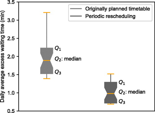
Results are summarized in Table 5 where the Tukey boxplot convention is utilized (plotting the lowest datum still within 1.5 the interquartile range (IQR) of the lower quartile, and the highest datum still within 1.5 IQR of the upper quartile). Table 5 demonstrates the improvement when using periodic rescheduling in the presence of different link travel time disturbances.

Table 5. Daily excess waiting time (min).

		Max	Q1	Median	Q3	Min	Median improvement
Scenario 1	Follow planned schedule	0.53	0.44	0.41	0.38	0.34
10% noise	Periodic rescheduling	0.44	0.34	0.33	0.27	0.22	19.5%
Scenario 2	Follow planned schedule	0.91	0.73	0.61	0.53	0.42
20% noise	Periodic rescheduling	0.77	0.54	0.44	0.32	0.26	27.9%
Scenario 3	Follow planned schedule	1.94	1.57	1.36	1.21	0.97
30% noise	Periodic rescheduling	1.16	0.97	0.81	0.63	0.52	40.4%
Scenario 4	Follow planned schedule	3.21	2.23	1.89	1.53	1.39
40% noise	Periodic rescheduling	1.50	1.28	0.98	0.71	0.69	48.2%

Testing the performance of the periodic rescheduling when the standard deviation is 10% of the expected value of the corresponding link travel time, one can observe that the mean benefit is reduced to 19.5%. Simulations show that the significance of periodic rescheduling increases when the variation of the actual link travel times from their expected values increases (for a standard deviation of 20% the EWT improvement becomes 27.9% and for 30% becomes 40.4%). Specific attention is given in the case of strong travel time disturbances (where the standard deviation of the normal distribution from which the travel times are sampled is 40% of the expected link travel times). This case is plotted in Figure 9 and shows a potential EWT improvement of 48.2%.

Figure 9. Tukey boxplot of the performance of the do-nothing scenario that follows the originally planned timetable and the periodic rescheduling in 15-min intervals.

Finally, we report in our discussion that during the daily operations one of the scheduled trips might be canceled. Given the time frame of our optimization though, any trip cancelation can be accounted for in the next rolling horizon. This can be achieved in our model by re-indexing the trips in the mathematical program of Equation (16)(16) $$\begin{array}{c}\underset{\mathbf{x}}{\text{argmin}}p(\mathbf{x})=f(\mathbf{x})+\sum _{i=1}^{\left|N\right|+\left|N\right|\left|S\right|}{W}_i{(\text{min}[0,c_i(\mathbf{x})])}^2\\ \mathrm{s}.\mathrm{t}. \hspace{0.17em}{x}_i=\{\begin{array}{c}{x}_i\in Q \text{if} a_{i,1}=0\hfill \\ x_i=0 \text{otherwise}\hfill \end{array}\\ {\beta }_{i,j}(\mathbf{x})={\beta }_{i,j-1}(\mathbf{x})-{\nu }_j{\beta }_{i,j-1}(\mathbf{x})+{\lambda }_{\rho ,j}[\left(d_{i,j}(\mathbf{x})+k_{i,j}(\mathbf{x})\right)-\left(d_{i-1,j}(\mathbf{x})+k_{i-1,j}(\mathbf{x})\right)],\\ \hspace{1em} \forall i\in N\setminus \left\{1\right\},j\in S\setminus \left\{1\right\} \text{where} d_{i,j}(\mathbf{x})\in \rho -\text{th} \text{hour}\\ {\beta }_{1,j}(\mathbf{x})={\beta }_{1,j-1}(\mathbf{x})-{\nu }_j{\beta }_{1,j-1}(\mathbf{x})+{\tilde{b}}_j, \forall j\in \{2,\dots ,|S\left|\right\}\\ {\beta }_{i,1}(\mathbf{x})={\lambda }_{\rho ,1}[\left(d_{i,1}(\mathbf{x})+k_{i,1}(\mathbf{x})\right)-\left(d_{i-1,1}(\mathbf{x})+k_{i-1,1}(\mathbf{x})\right)], \forall i\in N\setminus \left\{1\right\}\wedge d_{i,1}(\mathbf{x})\in \rho -\text{th} \text{hour}\\ {\beta }_{1,1}(\mathbf{x})={\tilde{b}}_1\\ d_{i,j}(\mathbf{x})=\{\begin{array}{cc}{a}_{i,j},\hfill & \text{if}{a}_{i,j}\ne 0\hfill \\ e_{i,j}(\mathbf{x}),\hfill & \text{otherwise}\hfill \end{array}\\ e_{i,j}(\mathbf{x})=({\delta }_i+x_i)+\sum _{\varphi =1}^{j-1}{t}_{i,\varphi }+\sum _{\varphi =1}^{j-1}{k}_{i,\varphi }(\mathbf{x})\\ k_{i,j}(\mathbf{x})={\eta }_1{\lambda }_{\rho ,j}\left[d_{i,j}(\mathbf{x})-d_{i-1,j}(\mathbf{x})\right]+{\eta }_2{\nu }_j{\beta }_{i,j-1}(\mathbf{x}),\forall i\in N\setminus \left\{1\right\},\forall j\in S\setminus \left\{1\right\}\\ k_{i,1}(\mathbf{x})={\eta }_1{\lambda }_{\rho ,1}\left[d_{i,1}(\mathbf{x})-d_{i-1,1}(\mathbf{x})\right],\forall i\in N\setminus \left\{1\right\}\\ Q=\{-30,-29,\dots ,0,\dots ,+29,+30\} \text{min}.\end{array}$$(16) prior to applying our solution method.

6. Concluding remarks

This article models the bus rescheduling problem in rolling horizons considering the vehicle capacity and the layover constraints. After the formulation of the periodic rescheduling problem as an integer nonlinear programing problem, it is proved that the problem complexity is exponential. This impedes the solution of the problem with analytical methods. Due to that, the constrained optimization problem is approximated with the use of exterior point penalties and a SHC solution method is developed to minimize the value of the resulting penalty function by exploring more efficiently the vast solution space.

This heuristic search method reduces the exponential computational complexity to polynomial and enables the rescheduling of the dispatching times of the remaining daily trips of a bus line at each rolling horizon instance. Applying the periodic rescheduling to bus line 15 L in Denver demonstrated a $\simeq$ 50% potential improvement of the daily average EWTs of passengers. This service regularity improvement is scenario-specific. For this reason, we study the sensitivity of the regularity improvement with periodic rescheduling for different levels of travel time disturbances. The results of the simulation-based sensitivity analysis show that if the daily operations are close to normal, periodic optimization offers a $\simeq 20\%$ margin of improvement. In contrary, if the AATs of buses at stops differ significantly from the expected ones, periodic optimization can offer higher gains in the range of 40–50%.

One important topic for future research is the consideration of multiple KPIs during the periodic rescheduling, such as the bus occupancy levels and the unsatisfied demand. Especially nowadays, the availability of smartcard data can be used to support this research topic and expand the EWT KPI by offering a more holistic view that considers both the service regularity and the passenger demand satisfaction as suggested by Randall, Condry, Trompet, and Campus (2007). Additionally, future research can investigate further the coordination between passenger arrival times and bus arrival times in high-frequency services because passengers that have access to real-time information on their mobile phones might try to synchronize the timing of their arrivals even if their expected waiting times are low.

Appendix A.

Genetic algorithm description

A typical genetic algorithm (GA) contains a number of strings which form the population at each of the iterations. Each string is a population member (individual) and represents a potential solution to the optimization problem. In our case, each population member m is a $\left|N\right|-$ valued vector of potential values of the decision variable $\{x_1,x_2,\dots ,x_{\left|N\right|}\}$ that determine the dispatching time modifications of all daily trips.

At the initialization stage of the GA, we should decide about the population size, $\left|P\right|,$ which is a hyperparameter of the GA. This parameter can be determined based on the tradeoff between solution space exploration and computational cost since a GA with a larger population size is expected to conduct a more comprehensive exploration of the solution space but requires also more time to evaluate all possible solutions.

Each population member, $\mathbf{m}\in P,$ is a vector $\mathbf{m}=(m_1,\dots ,m_i,\dots ,m_{\left|N\right|})$ with $\left|N\right|$ elements (known as genes) where each element $m_i\in \mathbf{m}$ represents the dispatching deviation of the i-th bus trip from its scheduled dispatching time. Each gene $m_i\in \mathbf{m}$ of an individual m is allowed to take an integer value from the set Q or is set equal to zero if bus trip $i\in N$ is already dispatched when the current re-scheduling occurs.

Therefore, a random initial population P can be generated as follows:

 For $\mathbf{m}=1$ to $\left|P\right|$

  For i = 1 to $\left|N\right|$

   If $a_{i,1}\ne 0:$ $m_i\leftarrow \mathit{random}.\mathit{choice}(Q)$

   If $a_{i,1}=0:$ $m_i\leftarrow 0$

  Next i

 Next m

GAs are typically designed to maximize fitness. Notwithstanding this, given the fact that our problem of Equation (16)(16) $$\begin{array}{c}\underset{\mathbf{x}}{\text{argmin}}p(\mathbf{x})=f(\mathbf{x})+\sum _{i=1}^{\left|N\right|+\left|N\right|\left|S\right|}{W}_i{(\text{min}[0,c_i(\mathbf{x})])}^2\\ \mathrm{s}.\mathrm{t}. \hspace{0.17em}{x}_i=\{\begin{array}{c}{x}_i\in Q \text{if} a_{i,1}=0\hfill \\ x_i=0 \text{otherwise}\hfill \end{array}\\ {\beta }_{i,j}(\mathbf{x})={\beta }_{i,j-1}(\mathbf{x})-{\nu }_j{\beta }_{i,j-1}(\mathbf{x})+{\lambda }_{\rho ,j}[\left(d_{i,j}(\mathbf{x})+k_{i,j}(\mathbf{x})\right)-\left(d_{i-1,j}(\mathbf{x})+k_{i-1,j}(\mathbf{x})\right)],\\ \hspace{1em} \forall i\in N\setminus \left\{1\right\},j\in S\setminus \left\{1\right\} \text{where} d_{i,j}(\mathbf{x})\in \rho -\text{th} \text{hour}\\ {\beta }_{1,j}(\mathbf{x})={\beta }_{1,j-1}(\mathbf{x})-{\nu }_j{\beta }_{1,j-1}(\mathbf{x})+{\tilde{b}}_j, \forall j\in \{2,\dots ,|S\left|\right\}\\ {\beta }_{i,1}(\mathbf{x})={\lambda }_{\rho ,1}[\left(d_{i,1}(\mathbf{x})+k_{i,1}(\mathbf{x})\right)-\left(d_{i-1,1}(\mathbf{x})+k_{i-1,1}(\mathbf{x})\right)], \forall i\in N\setminus \left\{1\right\}\wedge d_{i,1}(\mathbf{x})\in \rho -\text{th} \text{hour}\\ {\beta }_{1,1}(\mathbf{x})={\tilde{b}}_1\\ d_{i,j}(\mathbf{x})=\{\begin{array}{cc}{a}_{i,j},\hfill & \text{if}{a}_{i,j}\ne 0\hfill \\ e_{i,j}(\mathbf{x}),\hfill & \text{otherwise}\hfill \end{array}\\ e_{i,j}(\mathbf{x})=({\delta }_i+x_i)+\sum _{\varphi =1}^{j-1}{t}_{i,\varphi }+\sum _{\varphi =1}^{j-1}{k}_{i,\varphi }(\mathbf{x})\\ k_{i,j}(\mathbf{x})={\eta }_1{\lambda }_{\rho ,j}\left[d_{i,j}(\mathbf{x})-d_{i-1,j}(\mathbf{x})\right]+{\eta }_2{\nu }_j{\beta }_{i,j-1}(\mathbf{x}),\forall i\in N\setminus \left\{1\right\},\forall j\in S\setminus \left\{1\right\}\\ k_{i,1}(\mathbf{x})={\eta }_1{\lambda }_{\rho ,1}\left[d_{i,1}(\mathbf{x})-d_{i-1,1}(\mathbf{x})\right],\forall i\in N\setminus \left\{1\right\}\\ Q=\{-30,-29,\dots ,0,\dots ,+29,+30\} \text{min}.\end{array}$$(16) is casted as a minimization problem, in our study a population member m is considered more fit when its fitness function value, $p(\mathbf{m}),$ is lower.

In the parent selection stage, the fittest population members (individuals) are selected for reproduction and they pass their genes to the next generation. This is achieved by using the well-known roulette-wheel selection method (Goldberg & Deb, 1991). In the roulette-wheel selection method, each individual m has a probability of being selected which is proportional to its fitness value divided by the fitness values of all other population members. The parent selection process is repeated until the number of parents which are selected for reproduction is the same as the population size $\left|P\right|.$

At the crossover stage, two parents exchange their genes at a randomly selected crossover point selected from the set $\{1,2,\dots ,|N\left|\right\}$ for generating two offsprings. For instance, if the crossover point of two parents $\mathbf{m}=(m_1,\dots ,m_i,m_{i+1},\dots ,m_{\left|N\right|})$ and $\mathbf{m}\prime =(m{\prime }_1,\dots ,m{\prime }_i,m{\prime }_{i+1},\dots ,m{\prime }_{\left|N\right|})$ is $i\in N;$ then, the two generated offsprings will have the set of genes $(m_1,\dots ,m_i,m{\prime }_{i+1},\dots ,m{\prime }_{\left|N\right|})$ and $(m{\prime }_1,\dots ,m{\prime }_i,m_{i+1},\dots ,m_{\left|N\right|}).$

After the crossover stage follows the mutation stage. The mutation can be potentially applied to any generated offspring after the crossover stage. In our case, we specify a small probability, p_c, for replacing each gene of the generated offspring with a random value from the set Q.

The procedure described above continues iteratively until a pre-determined number of population generations, μ^max, is reached. The population member with the best performance is then selected as the final solution.

Note that the number of population members, $\left|P\right|,$ the mutation rate, p_c, and the maximum number of population generations, μ^max, are hyperparameters of the GA which should be externally defined and can affect the performance of the computed solution. For this reason, finding the most suitable hyperparameter values requires to optimize the same scenario multiple times with different hyperparameter values at each optimization.

References

- Aboudolas, K., Papageorgiou, M., Kouvelas, A., & Kosmatopoulos, E. (2010). A rolling-horizon quadratic-programming approach to the signal control problem in large-scale congested urban road networks. Transportation Research Part C: Emerging Technologies, 18(5), 680–694. doi:10.1016/j.trc.2009.06.003
- Bartholdi, J. J., & Eisenstein, D. D. (2012). A self-coördinating bus route to resist bus bunching. Transportation Research Part B: Methodological, 46(4), 481–491. doi:10.1016/j.trb.2011.11.001
- Berrebi, S. J., Hans, E., Chiabaut, N., Laval, J. A., Leclercq, L., & Watkins, K. E. (2018). Comparing bus holding methods with and without real-time predictions. Transportation Research Part C: Emerging Technologies, 87, 197–211. doi:10.1016/j.trc.2017.07.012
- Bertsekas, D. P. (1990). Nonlinear programming (2nd ed.). Belmont, MA: Athena Scientific.
- Bin, Y., Zhongzhen, Y., & Baozhen, Y. (2006). Bus arrival time prediction using support vector machines. Journal of Intelligent Transportation Systems, 10(4), 151–158. doi:10.1080/15472450600981009
- Calabrese, F., Di Lorenzo, G., Liu, L., & Ratti, C. (2011). Estimating origin-destination flows using opportunistically collected mobile phone location data from one million users in Boston Metropolitan Area. IEEE Pervasive Computing, 10(4), 36–44. doi:10.1109/MPRV.2011.41
- Cats, O., Larijani, A., Koutsopoulos, H., & Burghout, W. (2011). Impacts of holding control strategies on transit performance: Bus simulation model analysis. Transportation Research Record: Journal of the Transportation Research Board, 2216(1), 51–58. doi:10.3141/2216-06
- Cats, O., Larijani, A., Ólafsdóttir, Á., Burghout, W., Andreasson, I., & Koutsopoulos, H. (2012). Bus-holding control strategies: Simulation-based evaluation and guidelines for implementation. Transportation Research Record: Journal of the Transportation Research Board, 2274(1), 100–108. doi:10.3141/2274-11
- Cats, O., & Loutos, G. (2016). Real-time bus arrival information system: An empirical evaluation. Journal of Intelligent Transportation Systems, 20(2), 138–151. doi:10.1080/15472450.2015.1011638
- Ceder, A. (2007). “Public Transit Planning and Operation: Theory.” Modeling and practice. Oxford: Elsevier.
- Chang, H., Park, D., Lee, S., Lee, H., & Baek, S. (2010). Dynamic multi-interval bus travel time prediction using bus transit data. Transportmetrica, 6(1), 19–38. doi:10.1080/18128600902929591
- Chen, Q., Adida, E., & Lin, J. (2013). Implementation of an iterative headway-based bus holding strategy with real-time information. Public Transport, 4(3), 165–186. doi:10.1007/s12469-012-0057-1
- Chen, M., Liu, X., Xia, J., & Chien, S. I. (2004). A dynamic bus-arrival time prediction model based on APC data. Computer-Aided Civil and Infrastructure Engineering, 19(5), 364–376. doi:10.1111/j.1467-8667.2004.00363.x
- Chien, S. I.-J., Ding, Y., & Wei, C. (2002). Dynamic bus arrival time prediction with artificial neural networks. Journal of Transportation Engineering, 128(5), 429–438. doi:10.1061/(ASCE)0733-947X(2002)128:5(429)
- Chien, S. I.-J., & Kuchipudi, C. M. (2003). Dynamic travel time prediction with real-time and historic data. Journal of Transportation Engineering, 129(6), 608–616. doi:10.1061/(ASCE)0733-947X(2003)129:6(608)
- Cipriani, E., Gori, S., & Petrelli, M. (2012). Transit network design: A procedure and an application to a large urban area. Transportation Research Part C: Emerging Technologies, 20(1), 3–14. doi:10.1016/j.trc.2010.09.003
- Cortés, C. E., Sáez, D., Milla, F., Núñez, A., & Riquelme, M. (2010). Hybrid predictive control for real-time optimization of public transport systems’ operations based on evolutionary multi-objective optimization. Transportation Research Part C: Emerging Technologies, 18(5), 757–769. doi:10.1016/j.trc.2009.05.016
- Daganzo, C. F. (2009). A headway-based approach to eliminate bus bunching: Systematic analysis and comparisons. Transportation Research Part B: Methodological, 43(10), 913–921. doi:10.1016/j.trb.2009.04.002
- Dai, Z., Ma, X., & Chen, X. (2019). Bus travel time modelling using GPS probe and smart card data: A probabilistic approach considering link travel time and station dwell time. Journal of Intelligent Transportation Systems, 23(2), 175–190. doi:10.1080/15472450.2018.1470932
- Deb, K. (2001). Multi-objective optimization using evolutionary algorithms. Vol. 16. Chichester, UK: John Wiley & Sons.
- Eberlein, X. J., Wilson, N. H., & Bernstein, D. (2001). The holding problem with real–time information available. Transportation Science, 35(1), 1–18. doi:10.1287/trsc.35.1.1.10143
- Fan, W., & Machemehl, R. B. (2008). Tabu search strategies for the public transportation network optimizations with variable transit demand. Computer-Aided Civil and Infrastructure Engineering, 23(7), 502–520. doi:10.1111/j.1467-8667.2008.00556.x
- Farahani, R. Z., Miandoabchi, E., Szeto, W. Y., & Rashidi, H. (2013). A review of urban transportation network design problems. European Journal of Operational Research, 229(2), 281–302. doi:10.1016/j.ejor.2013.01.001
- Fiacco, A. V., & McCormick, G. P. (1968). Nonlinear programming: Sequential unconstrained minimization techniques. New York: John Wiley & Sons.
- Fortin, F.-A., Rainville, F.-M. D., Gardner, M.-A., Parizeau, M., & Gagné, C. (2012). DEAP: Evolutionary algorithms made easy. Journal of Machine Learning Research, 13, 2171–2175.
- Fu, L., & Yang, X. (2002). Design and implementation of bus-holding control strategies with real-time information. Transportation Research Record: Journal of the Transportation Research Board, 1791(1), 6–12. doi:10.3141/1791-02
- Gkiotsalitis, K. (2019). Robust stop-skipping at the tactical planning stage with evolutionary optimization. Transportation Research Record: Journal of the Transportation Research Board, 2673(3), 611–623. doi:10.1177/0361198119834549
- Gkiotsalitis, K., & Alesiani, F. (2019). Robust timetable optimization for bus lines subject to resource and regulatory constraints. Transportation Research Part E: Logistics and Transportation Review, 128, 30–51. doi:10.1016/j.tre.2019.05.016
- Gkiotsalitis, K., & Cats, O. (2018). Reliable frequency determination: Incorporating information on service uncertainty when setting dispatching headways. Transportation Research Part C: Emerging Technologies, 88, 187–207. doi:10.1016/j.trc.2018.01.026
- Gkiotsalitis, K., & Cats, O. (2019). Multi-constrained bus holding control in time windows with branch and bound and alternating minimization. Transportmetrica B: Transport Dynamics , 7(1), 1258–1285. doi:10.1080/21680566.2019.1606743
- Gkiotsalitis, K., Eikenbroek, O. A. L., & Cats, O. (2019). Robust network-wide bus scheduling with transfer synchronizations. IEEE Transactions on Intelligent Transportation Systems, 1–11. doi:10.1109/TITS.2019.2941847
- Gkiotsalitis, K., & Kumar, R. (2018). Bus operations scheduling subject to resource constraints using evolutionary optimization. Informatics, 5(1), 9. doi:10.3390/informatics5010009
- Gkiotsalitis, K., & Maslekar, N. (2018). Multiconstrained timetable optimization and performance evaluation in the presence of travel time noise. Journal of Transportation Engineering, Part A: Systems, 144(9), 04018058. doi:10.1061/JTEPBS.0000181
- Gkiotsalitis, K., & Maslekar, N. (2018). Towards transfer synchronization of regularity-based bus operations with sequential hill-climbing. Public Transport, 10(2), 335–361. doi:10.1007/s12469-018-0178-2
- Gkiotsalitis, K., & Stathopoulos, A. (2015). A utility-maximization model for retrieving users’ willingness to travel for participating in activities from big-data. Transportation Research Part C: Emerging Technologies, 58, 265–277. doi:10.1016/j.trc.2014.12.006
- Gkiotsalitis, K., Wu, Z., & Cats, O. (2019). A cost-minimization model for bus fleet allocation featuring the tactical generation of short-turning and interlining options. Transportation Research Part C: Emerging Technologies, 98, 14–36. doi:10.1016/j.trc.2018.11.007
- Goldberg, D. E., & Deb, K. (1991). A comparative analysis of selection schemes used in genetic algorithms. In Foundations of genetic algorithms, Vol. 1, 69–93. SanMateo, CA: Elsevier.
- Gurmu, Z., & Fan, W. (2014). Artificial neural network travel time prediction model for buses using only GPS data. Journal of Public Transportation, 17(2), 45. doi:10.5038/2375-0901.17.2.3
- Hickman, M. D. (2001). An analytic stochastic model for the transit vehicle holding problem. Transportation Science, 35(3), 215–237. doi:10.1287/trsc.35.3.215.10150
- Hounsell, N. B., Shrestha, B. P., & Wong, A. (2012). Data management and applications in a world-leading bus fleet. Transportation Research Part C: Emerging Technologies, 22, 76–87. doi:10.1016/j.trc.2011.12.005
- Ibarra-Rojas, O. J., Delgado, F., Giesen, R., & Muñoz, J. C. (2015). Planning, operation, and control of bus transport systems: A literature review. Transportation Research Part B: Methodological, 77, 38–75. doi:10.1016/j.trb.2015.03.002
- Jeong, R., & Rilett, R. (2004). Bus arrival time prediction using artificial neural network model. In Proceedings of the 7th International IEEE Conference on Intelligent Transportation Systems (IEEE Cat. No. 04TH8749, pp. 988–993). Washington, WA: IEEE.
- Karmarkar, N. (1984). A new polynomial-time algorithm for linear programming. In Proceedings of the sixteenth annual ACM symposium on Theory of computing, pp. 302–311. New York, NY: ACM.
- Kepaptsoglou, K., & Karlaftis, M. (2009). Transit route network design problem: Review. Journal of Transportation Engineering, 135(8), 491–505. doi:10.1061/(ASCE)0733-947X(2009)135:8(491)
- Koehler, L. A., Kraus, W., & Camponogara, E. (2011). Iterative quadratic optimization for the bus holding control problem. IEEE Transactions on Intelligent Transportation Systems, 12(4), 1568–1575. doi:10.1109/TITS.2011.2164909
- Kumar, B. A., Vanajakshi, L., & Subramanian, S. C. (2018). A hybrid model based method for bus travel time estimation. Journal of Intelligent Transportation Systems, 22(5), 390–406. doi:10.1080/15472450.2017.1378102
- Leong, W., Goh, K., Hess, S., & Murphy, P. (2016). Improving bus service reliability: The Singapore experience. Research in Transportation Economics, 59, 40–49. doi:10.1016/j.retrec.2016.07.025
- Leontitsis, A., Bountis, T., & Pagge, J. (2004). An adaptive way for improving noise reduction using local geometric projection. Chaos: An Interdisciplinary Journal of Nonlinear Science, 14(1), 106–110. doi:10.1063/1.1622354
- Mazloumi, E., Rose, G., Currie, G., & Sarvi, M. (2011). An integrated framework to predict bus travel time and its variability using traffic flow data. Journal of Intelligent Transportation Systems, 15(2), 75–90. doi:10.1080/15472450.2011.570109
- Pangilinan, C., Wilson, N., & Moore, A. (2008). Bus supervision deployment strategies and use of real-time automatic vehicle location for improved bus service reliability. Transportation Research Record: Journal of the Transportation Research Board, 2063(1), 28–33. doi:10.3141/2063-04
- Pelletier, M.-P., Trépanier, M., & Morency, C. (2011). Smart card data use in public transit: A literature review. Transportation Research Part C: Emerging Technologies, 19(4), 557–568. doi:10.1016/j.trc.2010.12.003
- Randall, E. R., Condry, B. J., Trompet, M., & Campus, S. K. (2007). International bus system benchmarking: Performance measurement development, challenges, and lessons learned. In Transportation Research Board 86th Annual Meeting, 21st–25th January. Washington, DC.
- Shalaby, A., & Farhan, A. (2004). Prediction model of bus arrival and departure times using AVL and APC data. Journal of Public Transportation, 7(1), 41. doi:10.5038/2375-0901.7.1.3
- Shen, Y., Xu, J., & Zeng, Z. (2016). Public transit planning and scheduling based on AVL data in China. International Transactions in Operational Research, 23(6), 1089–1111. doi:10.1111/itor.12164
- Smilowitz, K., Daganzo, C., Cassidy, M. J., & Bertini, R. L. (1999). Some observations of highway traffic in long queues. Transportation Research Record: Journal of the Transportation Research Board, 1678(1), 225–233. doi:10.3141/1678-27
- TfL. (2017). “Transport for London: Bus Routes and Borough Reports.” Retrieved from https://www.tfl.gov.uk/forms/14144.aspx.
- Transportation Research Group, University of Southampton. (1997). Bus Priority at Signals: AVL/BUS PRIORITY Headway Algorithm. Final Report to London Transport Buses, PRO 310. Technical Report. Transportation Research Group, University of Southampton.
- Trompet, M., Liu, X., & Graham, D. (2011). Development of key performance indicator to compare regularity of service between urban bus operators. Transportation Research Record: Journal of the Transportation Research Board, 2216(1), 33–41. doi:10.3141/2216-04
- van Hinsbergen, C. I., Van Lint, J. W. C., & Van Zuylen, H. J. (2009). Bayesian committee of neural networks to predict travel times with confidence intervals. Transportation Research Part C: Emerging Technologies, 17(5), 498–509. doi:10.1016/j.trc.2009.04.007
- Van Lint, J. W. C., Hoogendoorn, S. P., & van Zuylen, H. J. (2005). Accurate freeway travel time prediction with state-space neural networks under missing data. Transportation Research Part C: Emerging Technologies, 13(5-6), 347–369. doi:10.1016/j.trc.2005.03.001
- Van Oort, N., Wilson, N., & Van Nes, R. (2010). Reliability improvement in short headway transit services: Schedule-and headway-based holding strategies. Transportation Research Record: Journal of the Transportation Research Board, (2143(1), 67–76. doi:10.3141/2143-09
- Vlahogianni, E. I., Karlaftis, M. G., & Golias, J. C. (2005). Optimized and meta-optimized neural networks for short-term traffic flow prediction: A genetic approach. Transportation Research Part C: Emerging Technologies, 13(3), 211–234. doi:10.1016/j.trc.2005.04.007
- Welding, P. I. (1957). The instability of a close-interval service. Journal of the Operational Research Society, 8(3), 133–142. doi:10.1057/jors.1957.21
- Xuan, Y., Argote, J., & Daganzo, C. F. (2011). Dynamic bus holding strategies for schedule reliability: Optimal linear control and performance analysis. Transportation Research Part B: Methodological, 45(10), 1831–1845. doi:10.1016/j.trb.2011.07.009
- Yan, Y., Liu, Z., Meng, Q., & Jiang, Y. (2013). Robust optimization model of bus transit network design with stochastic travel time. Journal of Transportation Engineering, 139(6), 625–634. doi:10.1061/(ASCE)TE.1943-5436.0000536
- Yu, B., Lam, W. H., & Lam Tam, M. (2011). Bus arrival time prediction at bus stop with multiple routes. Transportation Research Part C: Emerging Technologies, 19(6), 1157–1170. doi:10.1016/j.trc.2011.01.003
- Yu, B., Wang, H., Shan, W., & Yao, B. (2018). Prediction of bus travel time using random forests based on near neighbors. Computer-Aided Civil and Infrastructure Engineering, 33(4), 333–350. doi:10.1111/mice.12315
- Yu, B., Yang, Z.-Z., Chen, K., & Yu, B. (2010). Hybrid model for prediction of bus arrival times at next station. Journal of Advanced Transportation, 44(3), 193–204. doi:10.1002/atr.136
- Zaki, M., Ashour, I., Zorkany, M., & Hesham, B. (2013). Online bus arrival time prediction using hybrid neural network and Kalman filter techniques. International Journal of Modern Engineering Research, 3(4), 2035–2041.