Modelling dry season deciduousness in Mexican Yucatán forest using MODIS EVI data (2000–2011)

Abstract

This study maps interannual variation in the spatial extent of deciduousness in the dry tropical forests of the southern Yucatán (Mexico) from 2000 to 2011 using seasonal variability thresholds based on Moderate Resolution Imaging Spectroradiometer (MODIS) Enhanced Vegetation Index (EVI) data and relates deciduousness to precipitation- and temperature-derived climate variables using linear regressions. The annual occurrence of deciduousness is most frequently observed in forests located in a regional rain shadow at moderate elevations. Regression results suggest that deciduousness is more strongly associated with atypically hot conditions (–2°C; R ² = 0.44) than with atypically dry conditions (R ² = 0.19), in contrast to other phenological processes (e.g. leaf growth, peak productivity) driven primarily by precipitation.

Keywords:

• phenology
• deciduousness
• MODIS

1. Introduction

Although much attention has been paid to the condition of moist tropical forests since the speed of forest conversion became appreciated in the late twentieth century (Myers 1984; Skole and Tucker 1993), fewer studies have addressed deforestation and degradation of deciduous or semi-deciduous dry tropical forests (Mooney, Bullock, and Medina 1995; Pennington, Prado, and Pendry 2000). This disparity is significant given that dry tropical forests comprise 42% of all tropical forests (Murphy and Lugo 1986; Janzen 1988) and harbour large numbers of endemic species (Ceballos and Brown 1995; Trejo and Dirzo 2000). The dry tropical forests of the Yucatán region are the last remaining frontier forest tracts in Mexico and are subject to competing tensions of habitat conservation versus economic development (Turner, Geoghegan, and Foster 2004). Changes to the intensity and spatial extent of the seasonal phenomenon of deciduous leaf drop, referred to here as deciduous phenology, have the potential to determine future wildlife habitat quality, soil composition, and energy transfer in the region (Holbrook, Whitbeck, and Mooney 1995; Lawrence 2005). The importance of phenology as a regional determinant of ecosystem functioning may increase as high regional rates of deforestation observed from 1960 to 1993 have declined on account of forest conservation and reduced in-migration of human populations (Turner, Geoghegan, and Foster 2004; Rueda 2010). Furthermore, this phenology may be altered with a changing climate.

Dry tropical forests are defined globally by annual precipitation of 250–2000 mm during a wet season of 4–9 months (Murphy and Lugo 1995). Many tree species in dry tropical forests exhibit deciduous leaf abscission, a behavioural adaptation to avoid negative leaf carbon balance and desiccation of stem tissue (Borchert 1994; Holbrook, Whitbeck, and Mooney 1995). The temporal and spatial variability in deciduous intensity can be substantial, ranging from 25% to 100% of leaves lost in a single dry season per unit area (Lawrence 2005). Local physiological characteristics of organisms, species, and life-forms and regional environmental factors such as elevation, temperature, and the magnitude and seasonal distribution of precipitation have all been identified as factors that potentially determine the timing, location, and amount of deciduous leaf loss (Whigham et al. 1990; Borchert 1994; Holbrook, Whitbeck, and Mooney 1995). Still, the relative importance of the physiological and environmental drivers of deciduousness has been observed to vary among different dry tropical forest ecosystems (Holbrook, Whitbeck, and Mooney 1995; Zhang et al. 2005) and different temporal extents (Whigham et al. 1990).

The mechanisms through which climate and weather conditions lead to dry tropical deciduousness are understood only broadly. Water availability to dry tropical forest vegetation is mediated by the amount of precipitation over recent weeks or months, the regularity of precipitation events, and the rate of water runoff and soil drainage (Whigham et al. 1990; Condit et al. 2000; Chapin, Matson, and Mooney 2002). Water drains quickly through the permeable, karstic soils of the Yucatán (Querejeta et al. 2007), and water availability may be expected to correlate strongly with the amount and frequency of recent precipitation (Whigham et al. 1990). High daytime surface temperature increases the water potential difference between tree roots and atmosphere as well as potential evapotranspiration, resulting in greater water loss through leaf stomata and from the soil (Chapin, Matson, and Mooney 2002). The relationship between temperature and phenology in dry tropical forests is typically viewed as secondary to the relationship between precipitation and phenology because temperature, unlike precipitation, is not a defining characteristic of the biome (Mooney, Bullock, and Medina 1995), and the influence of temperature on dry tropical deciduous phenology has not been analysed at the regional scale. Finally, physiological characteristics of vegetation related to absorbing and holding water (e.g. the extent and depth of root systems, regulation of stomata, cell elasticity) determine the degree to which low water availability constitutes plant water stress and introduce spatial variability in the relationship between environmental conditions and deciduousness (Mooney, Bullock, and Medina 1995; Borchert 1999; Chapin, Matson, and Mooney 2002).

Increases in the extent, duration, and intensity of deciduousness may lessen the effectiveness of local conservation efforts in Yucatán dry forests by restricting local faunal habitat quality (Bohlman 2010) and affecting floral species assemblages by altering nutrient inputs (e.g. N, P) to the soil (Condit et al. 2000, 2004; Lawrence 2005; Bohlman 2010). Seasonal and interannual phenological variations affect the habitat ranges of fauna such as the white-lipped peccary (Tayassu pecari) (Reyna-Hurtado, Rojas-Flores and Tanner, 2009) and the white-nosed coati (Nasua narica) (Valenzuela and Ceballos 2000) by limiting available food sources. Deciduousness also transfers organic matter from tree canopies to soils, potentially priming soil decomposition and ultimately transmitting carbon to the atmosphere (Vitousek and Sanford 1986; Chapin, Matson, and Mooney 2002). A thinner canopy facilitates foraging by pollinator species (e.g. stingless bee, Trigona fulviventris) and increases understory insolation, enabling the growth potential of understory vegetation (Hartshorn 1988; Chapin, Matson, and Mooney 2002) and leading to drier ground fuels and increased wildfire susceptibility (Nepstad et al. 1995). Increased knowledge of interannual variability in the spatial extent and intensity of deciduousness and of the relationship between environmental conditions and deciduousness allows more accurate forecasting of impacts related to ongoing conservation efforts, or to wildfire risk, in the region.

This article is motivated by the need to characterize temporal and spatial trends and variability of dry season deciduousness in the Mexican Yucatán Peninsula and to examine the degree to which climate variables influence deciduousness. The specific objectives are as follows:

1.

Map the spatiotemporal variability of deciduous phenology using image metrics derived from monthly 1 × 1 km2 Moderate Resolution Imaging Spectroradiometer (MODIS) Enhanced Vegetation Index (EVI) data (MOD13A3) captured from 2000 to 2011 and characterize the environmental conditions on which the extent of deciduousness depends.

2.

Assess the environmental conditions associated with deciduousness through examination of spatial and temporal variability in the relationship between climate variables and vegetation phenology using linear regressions of monthly EVI data against data derived from monthly Tropical Rainfall Measuring Mission (TRMM) 34B3 precipitation (0.25 × 0.25 degrees) and monthly MOD11C3 Land Surface Temperature (LST) (0.05 × 0.05 degrees).

1.1. Background: remote sensing of vegetation phenology

Over the last decade, the practice of monitoring vegetation phenology at landscape or at regional scales has become popular due in large part to the maturation of land remote sensing (Ustin 2004) and the increased availability of ground monitoring systems (Richardson et al. 2007). This practice, referred to as ‘land surface phenology,’ relies on remote sensing instruments (e.g. NOAA AVHRR, MODIS) that capture imagery at a moderate spatial resolution (i.e. from 100 × 100 to 1000 × 1000 m²) to monitor the amount of photosynthetically productive vegetation over broad areas and to derive metrics and dates of interest related to plant life cycles (Morisette et al. 2009; de Beurs and Henebry 2010). Numerous phenological studies have developed metrics, thresholds or data-derived frameworks that rely on remotely sensed proxies of vegetation to examine phenological patterns over a spatially continuous, broad scale (Tateishi and Ebata 2004; Xiao et al. 2006; Ito et al. 2008; Swain et al. 2011).

A number of studies have investigated phenological variability in dry tropical or subtropical forest to relate deciduousness to proximal environmental conditions (Table 1). Xiao et al. (2006) measured the timing of peak EVI, value of peak EVI, start of dry season, and end of dry season in the Amazon basin in 2002 to examine the potential climatic drivers of phenology. EVI peaks were detected during the late dry season and early wet season, suggesting that solar irradiation may be the primary driver of phenology in a large portion of Amazon evergreen forests. Park (2010) measured spatial variability in the value and date of peak greenness using Normalized Difference Vegetation Index (NDVI), EVI and the temporal distribution of precipitation in the tropical Hawaiian ecosystems and found that the timing of peak greenness occurred during the dry season for forests that received high annual rainfall (>3000 mm/year) and during the wet season for forests that received low annual rainfall. Additionally, variability of phenology across forest types has been investigated in subtropical ecosystems. Ito et al. (2008) used 1 × 1 km² advanced very high resolution radiometer (AVHRR) NDVI data to map the amount of photosynthetically active canopy in a Cambodian dry tropical forest between May 2001 and April 2002. By breaking annual trends of NDVI into a series of best-fit harmonic curves, the work distinguished deciduous forest from non-deciduous forest locations on the basis of the number of local EVI minima in the annual phenological cycle and further classified deciduous forests according to the part of the annual cycle during which they exhibit deciduousness (Ito et al. 2008).

Table 1. Summary of land surface phenology studies.

Study area	Temporal extent	Sensor	Temporal Res.	Spatial Res.	Measurement of phenology	Relation to climate	Study
Southern Amazon Basin	2002	MODIS	16 day	250 m	EVI observations were compared to vegetation fraction (VF) estimates from spectral mixture analysis	Linear regression relating EVI and VF to precipitation	Anderson et al. (2011)
North Carolina, USA	2001–2008	MODIS	16 day	250 m	Logistic functions fit to seasonal LAI change and phenological metrics extracted at fitted maxima and inflection points	Linear regression relating phenological dates to topographic variables	Hwang et al. (2011)
Hawai'i, USA	2006–2007	MODIS	16 day	250 m	Seasonal cycles of EVI and NDVI decomposed into harmonic terms	Amplitude of largest harmonic term compared across different rainfall regime extents	Park (2010)
Cambodia	2001–2002	AVHRR	10 day	1 km	Extraction of dates of local NDVI maxima and minima	Temporal correspon- dence of max./min. NDVI and dry season	Ito et al. (2008)
Amazon Basin	2002	MODIS	8 day	500 m	Seasonal EVI change	Temporal correspon- dence of peak EVI and dry season	Xiao et al. (2006)
Global	1982–2000	AVHRR	10 day	8 km	Seasonal NDVI change	Linear regression relating NDVI to LST, Precip.	Tateishi and Ebata (2004)
Kansas, USA	1989–1997	AVHRR	14 day	1.1 km	Seasonal NDVI change	Linear regression relating NDVI to Temperature., Precip.	Wang et al. (2001)

The potential bio-climatic drivers of phenology are frequently examined in land surface phenology studies, and linear regressions are typically employed to describe the strength and significance of relationships between deciduousness and its potential drivers. The relative and absolute impact of individual drivers and the temporal scales at which their impact can be detected have been seen to vary across ecosystem type. Tateishi and Ebata (2004) analysed global phenological patterns from 1982 to 2000 using 8 × 8 km² NOAA AVHRR data and 0.5 × 0.5 degree Climate Research Unit LST data and observed a negative relationship between NDVI and LST in subtropical areas of Central America, though strong positive correlation was seen between temperature and NDVI in other tropical forest ecosystems. Hwang et al. (2011) examined the effect of topographic controls on the timing of phenological events in a hilly, forested watershed in North Carolina, USA, using MODIS 250 × 250 m² NDVI and Leaf Area Index (LAI) products and found that elevation, aspect and solar irradiance potential had substantial and significant explanatory power with respect to the timing of leaf growth and senescence. Anderson et al. (2011) found MODIS EVI to be sensitive to changes in the forest canopy in the southern Amazon for both vegetation growth and senescence, but did not observe a significant relationship between EVI and precipitation, although rainfall in the study area was highly spatially variable (1200–2750 mm/year) and seasonally concentrated.

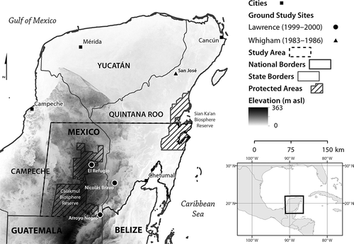
Two ground studies of deciduousness in the Yucatán examined the relationship between the timing and amount of deciduousness and contextual factors such as precipitation and forest age. Lawrence (2005) examined litterfall at three sites near the Calakmul Biosphere Reserve, of various successional states, in the southern Yucatán along a precipitation gradient during the historically wet 1999 season (see location of sites in Figure 1). Lawrence (2005) observed the highest variability of litterfall (greatest relative peak in leaf loss, related to the degree of deciduousness) in the older and drier forest sites. The onset of deciduousness occurred earlier in forests that received greater annual rainfall, indicating that vegetation experienced water stress. Later onset of deciduousness in forests that received less annual rainfall indicated that forests were able to tolerate periods of low water availability. Whigham et al. (1990) monitored the relationship between litterfall and precipitation at a site in Quintana Roo during years 1984–1987 (see Figure 1). Whigham et al. (1990) observed significant correlation between annual precipitation and mass of litterfall, and the results suggest that vegetation at the study site could experience 1–2 months of little to no precipitation before exhibiting deciduousness, but that interannual variation in the total amount of annual precipitation did trigger significant change in the mass of litterfall. These two studies demonstrate that factors such as forest age, average annual precipitation and frequency of precipitation events influence the deciduous response to precipitation at the plot scale in the Yucatán. High spatial and interannual variability of deciduousness and its relationship to climate are observed within a relatively small study area. Similar factors may play a role observable at a coarser larger spatial scale (1 × 1 km²) across the region.

Figure 1. The Mexican Yucatán Peninsula, with study area indicated in red. Circle markers show approximate location of litter measurement by Lawrence (2005). Triangle marker shows the location of litter measurement by Whigham et al. (1990).

In contrast to other land surface phenology studies that have investigated dry tropical forests over one or two annual cycles, this article makes use of the complete available MODIS data series, capturing phenology over 11 annual cycles from 2000 to 2011, a comparatively long temporal extent that allows examination of substantial interannual variability in deciduousness. Also, a methodology specifically designed to examine the phenomenon of deciduousness, distinct from other phenological processes, is employed.

2. Methodology

2.1. Study area

This article examines dry season deciduousness within a 42,500 km² area in the Mexican Yucatán region, approximately 200 km north–south and extending 275 km inland west from the Caribbean coast to cover portions of the states Quintana Roo and Campeche (Figure 1). For the period of observation 2000–2011, the regional mean annual temperature was 27 °C and the mean precipitation ranged from 750 to 1350 mm/year. Rainfall exhibits a seasonal pattern, with a wet season from June to October and a dry season from November to May (Lawrence 2005). The eastern, near-coastal areas of the southern Yucatán receive higher annual precipitation (˜1500 mm/year) than upland areas to the west (˜1000 mm/year), and movement of weather systems typically follows an ESE to WNW path (Márdero and Silvia, 2011). For upland areas in the western part of the study area in the period 1965–2000, average annual precipitation in the wet season decreased to 4.63 mm/year (−0.6% per year, 22.1% total decline over period), and average annual precipitation in the dry season decreased to 0.35 mm/year (−0.3% per year, 12.8% total decline over period) (Márdero and Silvia, 2011). Regional topography is characterized by low slope areas along the coast and rolling limestone hills, interspersed with large solution sinks and seasonally inundated, short stature forest, referred to as bajos, located farther inland. A number of forest subtypes exist within the region, distinguished on the basis of their stature, topography and the tendency of common tree species to exhibit deciduousness (Pérez-Salicrup 2004). These types include selva baja (4–8 m stature, irregularly inundated), selva subcaducafolia (6–12 m, upland semi-deciduous), selva mediana (12–25 m, upland semi-evergreen), and selva alta (25 – m, upland semi-evergreen) (Schmook et al. 2011).

The region contains two federally protected reserves: Sian Ka'an Reserve on the Caribbean coast of Quintana Roo and the inland Calakmul Biosphere Reserve (in Campeche and Quintana Roo), both part of the Mesoamerican Biological Corridor (MBC), which runs along a north-south precipitation gradient connecting a series of reserves from southern Mexico to Panama (Vester et al. 2007). Deciduousness in the study area shows part of the broad-scale response of Central American forests to climatic trends and variability (Condit et al. 2000), exhibited by trees that predictably shed leaves seasonally and by trees that shed leaves only facultatively in times of substantial water stress. Tree species typical of mature forest in the study area include Brosimum alicastrum (ramón), Thouinia canescens, Bursera simaruba and Manilkara zapota (L.) (Pérez-Salicrup 2004).

2.2. Data

MODIS EVI and climate variables

Monthly EVI image composites from MODIS product MOD13A3 (1 × 1 km²) were compiled in an 11-year time series (2000–2011) to map the spatial and temporal variability of deciduous phenology (Table 2 ). The product is a monthly maximum value composite of observations made from the Terra platform that are geometrically corrected and distributed in a sinusoidal projection (Justice et al. 1998). Image compositing reduces the impact of cloud cover, low sun angle or other sources of atmospheric scattering such as smoke (Huete et al. 2002; Schaaf et al. 2002). Annual periods began in June to coincide with the typical start of wet season and to completely capture annual periods of vegetation senescence and deciduous leaf loss.

Table 2. Data used in the study.

Variable	Sensor/Source	Product name	Spatial resolution	Spatial extent in region	Static/dynamic	Temporal resolution/extent
EVI	MODIS Terra	MOD13A3	1 km	Full	Dynamic	Monthly, 2000–2011
Land surface temperature	MODIS Terra	MOD11C3	0.05 deg.	Full	Dynamic	Monthly, 2000–2011
Precipitation	TRMM	34B3	0.25 deg.	Full	Dynamic	Monthly, 2000–2011
Elevation	SRTM	DEM	90 m	Full	Static	2000
Deciduousness	Landsat TM, ETM–		30 m	Scene 20/47 (˜92 W to 86 W; 17 N to 20 N)	7 Dates (Unequally-spaced)	2009
Forest type/land cover	Landsat ETM–		30 m	Scenes 20/47 and 19/47	Static	2010

A time series of precipitation was derived from the TRMM product 3B43, the highest available spatial resolution remotely sensed estimates of global precipitation (Immerzeel, Rutten, and Droogers 2009), that are distributed as monthly composites of average hourly precipitation at a spatial resolution of 0.25 × 0.25 degrees (˜28 × 28 km²) (Huffman et al. 2007). A 1-month temporally lagged time series and a time series of average monthly rainfall over the preceding 3 months (after Whigham et al. 1990) were derived from the TRMM time series to account for potential stored subsurface water. The data were downscaled to 1 km using a nearest neighbour resampling method. LSTdata were derived from the MODIS 5.6 × 5.6 km² Terra product MOD11C3, monthly composites of average daytime temperature (Wan and Li 1997; Wan et al. 2004) that were downscaled to 1 × 1 km² using a nearest neighbour resampling method.

Landsat data

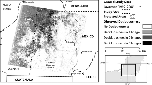
To assess the validity of MODIS-based indicators of deciduousness, reference maps of the spatial distribution of deciduousness were created from Landsat imagery. Three deciduousness maps derived from Landsat TM and ETM– images from the dry season in 2009 (path/row 20/47) indicate areas of deciduous forest in the western area of the study area. Data were captured on 16 February 2009, 4 March 2009, and 5 April 2009, during the dry season of a year, that is typical with respect to annual EVI variability in the total series (Figure 2). These three binary maps delineated the spatial extent of deciduousness based on the thresholds derived from Kauth–Thomas greenness and wetness (Kauth and Thomas 1976), were produced using the Mahalanobis Typicality algorithm (Foody 2002; Hernandez et al. 2008), and were validated using ground reference data (see Christman et al., forthcoming).

Figure 2. Seasonal deciduousness map created using a Mahalanobis Typicality threshold for deciduousness in three Landsat TM and ETM– scenes from 2009 (16 February, 4 March, and 5April).

Environmental variables

A 90 × 90 m² spatial resolution digital elevation model from the Shuttle Radar Topographic Mission (SRTM) (Farr et al. 2007) was used to assess the effect of topography on deciduousness (Hwang et al. 2011). A 30 × 30 m² spatial resolution Landsat-derived land cover map corresponding to 2010 was used to mask out non-forested land from analysis. The map was created using Landsat TM and ETM– images from two scenes, path/row 19/47 (captured 9 August 2010) and 20/47 (captured 10 January 2012), and covers nearly the entire study area.

2.2. Methods

Phenology and climate

Temporal profiles for EVI, LST and TRMM precipitation data are presented for data averaged over three regions: the entire study area and two 5 × 5 pixel forested target areas (˜21.5 km²). One of these 5 × 5 pixel areas exhibited strong and spatially clustered deciduousness in the 2009 dry season Landsat imagery, while the other area exhibited a negligible amount of deciduousness. Both target areas were chosen opportunistically to represent typical climate conditions in deciduous and non-deciduous forests. Temporal profiles of EVI and climate variables extracted in these two locations allow the characterization of vegetation and climate in deciduous and non-deciduous forests within the study area.

Characterization of deciduousness

Each pixel of the MODIS EVI data product contains a high number of individual trees that vary in the degree to which they exhibit deciduousness. Binary MODIS-based Deciduousness Dominance maps indicate which pixels comprised mostly of deciduous vegetation and were created for each year of the study. Deciduous vegetation was determined to be dominant in pixels where the annual range of EVI was greater than 50% of the annual maximum EVI (White and Nemani 2006):

Dominance of Deciduousness_year IF:

(1)

The threshold of 0.5 was chosen because it yielded a Dominance of Deciduousness mapthat corresponded strongly to the Landsat-based map of deciduousness for the 2009 dry season. When the accuracy of the 2009 Dominance of Deciduousness map was assessed using the Landsat-based deciduousness map as reference, agreement was demonstrated with an overall accuracy of 89% and with user's and producer's accuracies of 66% and 67%, respectively, for the presence of deciduousness class. The use of alternative thresholds to determine areas of deciduous dominance did not produce maps that corresponded as closely with the Landsat map of deciduousness.

The 11 annual binary MODIS Dominance of Deciduousness maps were aggregated to produce a single Frequency of Deciduousness map that shows the per-pixel frequency of observed deciduousness during the study period. Aggregated Dominance of Deciduousness data were simplified to four frequency classes, which show areas where deciduousness dominance was a recurrent seasonal phenomenon, where it was an occasional response to atypical conditions, and where it rarely or never occurred. The Frequency of Deciduousness classes show the following:

•	• Areas that were never observed to be deciduous dominant
•	• Areas that were observed to be low-frequency deciduous dominant (deciduous dominance in 1–2 years)
•	• Areas that were observed to be moderate-frequency deciduous dominant (deciduous dominance in 3–4 years), and
•	• Areas that were observed to be high-frequency deciduous dominant (deciduous dominance in 5 or more years).

Frequency of Deciduousness classes were delineated in this way to ensure that they are of a sufficiently large spatial extent, are of comparable size, and serve as areas over which representative summary statistics of vegetative vigour and climate variables could be extracted.

Deseasoning data

The process of deseasoning, also referred to as climatological standardization, standardizes the value of an observation with respect to the set of all observations from the same month in all years of the time series. This reduces serial correlation in the time series and highlights periods of unusually high or low amounts of photosynthetically active vegetation, temperature or precipitation. To calculate deseasoned values (standardized anomalies) for each time and pixel, the mean monthly value in the time series for each month was subtracted from each year's observed value in that month and divided by the standard deviation for the set of observations in that month, in all years of the time series (Nicholson and Entekhabi 1987):

(2)

Deseasoned time series of EVI, precipitation and LST were used as variables in one part of the regression analysis. In the remaining regressions, non-deseasoned time series were used, in which each observed monthly pixel value was differenced from the total series pixel mean value.

Linear regression

A number of univariate and multivariate linear regression models (ordinary least squares) were performed to estimate the best-fit linear model to describe the effect of environmental conditions on EVI and to measure the phenological variability in EVI that can be explained by select temperature- and precipitation-derived climate variables. These regression models varied with respect to the pre-processing of analysed time series (i.e. deseasoned/non-deseasoned), the temporal domain of input data, and the climate variable or variables examined. For univariate regressions, R ² was used as a measure of significance, and for bivariate regressions, adjusted R ² was used. The resulting set of regression equations distinguishes the environmental conditions associated with deciduousness from those associated with other phenological change (e.g. leaf growth), indicates the distinct spatial distributions of both seasonal and facultative deciduousness, and suggests the relative importance of individual climate variables as drivers of deciduousness.

The first model used non-deseasoned EVI to demonstrate the link between greenness and seasonal variation of precipitation or temperature and is referred to as the seasonal variability regression. Univariate linear regressions examined relationships between EVI (dependent variable) and one of the following independent variables: same-month LST, same-month precipitation, 1-month-lagged precipitation and total precipitation over the same and preceding 2 months. Lagged LST variables were examined, but did not correlate as strongly with EVI as same-month LST. A multivariate linear regression examined the relationship between EVI and both same-month LST and the most significant precipitation-derived variable.

The second model uses deseasoned EVI to examine the impact on greenness of short-term periods in which observed precipitation or temperature varies from observed mean values from 2000 to 2011. This model is referred to as the interannual variability regression, in reference to the climatological deseasoning of the data used. Univariate linear regressions examined deseasoned EVI (dependent variable) and one of the independent variables: same-month LST (deseasoned), same-month precipitation (deseasoned), 1-month-lagged precipitation (deseasoned) and total precipitation over the current and preceding 2 months (deseasoned). A multivariate linear regression examined the relationship between deseasoned EVI and both deseasoned same-month LST and the most significant precipitation-derived variable.

Seasonal variability and interannual variability regressions were run for two temporally different sets of observations. The first set includes all monthly observations from June 2000 to May 2011 (N = 132), and the results of these regressions characterize the full range of regional vegetation behaviour including growth, maturity, senescence and deciduousness. This set of regressions will be referred to as the total-time-series regressions. The second set of data includes only observations from the dry season months January through May from the year 2001 to 2011 (N = 55). This period was observed by Lawrence at three ground sites in the central part of the study area (Figure 1) to contain the times of peak leaf litter loss (˜75% of total annual litter), and the results of regressions that analyses only dry season observations offer refined characterization of the drivers of deciduousness. This set of regressions will be referred to as the dry-season-only regressions.

For all regression types, the per-pixel coefficients of determination (R ²) for each univariate linear regression were spatially averaged over the total study area and over each category extent in the Frequency of Deciduous Dominance map. Per-pixel significance was calculated using an analysis of variance F-statistic test for the two univariate regressions that explain EVI using temperature and using the best performing precipitation-derived independent variable. Maps are presented of per-pixel significance at the 1% and 0.1% level (Vincent et al. 2004). The Durbin–Watson statistical test was used to test each univariate regression for first-order serial auto-correlation at probability 0.01 (Durbin and Watson 1951). Subsequently, a multivariate linear regression that explains EVI using temperature and the best performing precipitation-derived independent variable is performed, and per-pixel adjusted coefficients of determination (adjusted R ²) are presented as maps and spatially averaged over the same extents as the univariate regression R ².

3. Results

3.1. Phenology and climate

A profile of EVI for the period 2000–2011, spatially averaged over the total study area, displays a clear seasonal pattern (Figure 3). The annual mean EVI is 0.53 and exhibits little interannual variability (interannual standard deviation = 0.010, 1.9% of the mean) but a greater amount of within year varitation (monthly standard deviations range from 0.05 to 0.07). Similar patterns with respect to seasonal and interannual variability are observed for temperature. The annual mean temperature is 26.2°C, with an interannual standard deviation of 0.4°C (0.15% of the mean) and monthly standard deviations ranging from 2.1°C to 3°C. Precipitation displays relatively high interannual variability in addition to seasonal variability. For the period 2000–2011, mean total annual precipitation is 1139 mm, with substantial and interannual variability (interannual standard deviation = 238 mm, 20.9% of the mean). Substantially, higher total annual precipitation is observed in the first half of the study than in the second half: mean total annual rainfall is 1352 mm for the years 2000–2005 and 949 mm for the years 2007–2011 (Table 3)

Table 3. EVI, precipitation, and temperature conditions observed during the study period, spatially extracted over the total study area (temp. = temporal).

	EVI			Precipitation mm/month			Temperature degrees C
Annual period (starting year):	Mean	Seasonal Range	Std. Dev. (temp., monthly)	Mean	Seasonal Range	Std. Dev. (temp., monthly)	Mean	Seasonal Range	Std. Dev. (temp., monthly)
2000	0.54	0.16	0.06	128	297	113	25.6	7.5	2.2
2001	0.55	0.16	0.05	108	259	78	25.8	6.4	2.1
2002	0.54	0.14	0.06	114	339	95	26.5	9.4	2.8
2003	0.52	0.18	0.06	114	207	67	26.3	9.0	2.5
2004	0.53	0.20	0.07	91	221	69	26.6	6.5	2.3
2005	0.51	0.19	0.06	84	145	57	26.3	8.2	2.9
2006	0.53	0.21	0.06	92	160	49	25.8	8.3	2.6
2007	0.53	0.13	0.05	77	145	47	26.3	8.0	2.6
2008	0.52	0.18	0.06	73	251	71	26.2	8.6	3.0
2009	0.51	0.14	0.05	77	121	36	26.7	8.0	2.7
2010	0.51	0.18	0.06	71	207	61	26.6	9.0	2.8
2000–2011	0.53	0.17	0.06	93	214	67	26.2	8.1	2.6
Std. Dev. (temp., interannual)	0.01	0.03	0.01	19	69	22	0.4	1.0	0.3

.

Figure 3. Temporal profile of monthly EVI, TRMM precipitation and MODIS land surface temperature spatially averaged over the entire study area (left) and in two ˜21.5 km² deciduous and non-deciduous target areas (right).

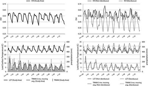
For the same period at the deciduous forest 5 × 5 pixel target area, the vegetation and climate profiles observed resemble those from the total study area, but exhibit an even stronger seasonal pattern (Figure 3). The deciduous forest target location has a substantially lower mean annual minimum EVI, lower total precipitation and higher temperature relative to the total study area (Figure 3). The same temporal distribution of precipitation is observed in the deciduous forest target area, with earlier years exhibiting greater total precipitation than the later years.

The non-deciduous forest 5 × 5 pixel target location exhibits climate seasonality that strongly resembles the pattern seen throughout the study area, but vegetation vigour exhibits relatively little seasonality (Figure 3). The non-deciduous forest target area has a lower mean annual minimum LST, and higher total precipitation, than either the deciduous target area or the total study area (Figure 3). The low canopy vegetation seasonality of this target area is reflected in the relationship between mean annual minimum EVI and mean annual maximum EVI. Relative to mean annual maximum EVI, mean annual minimum EVI is 24% lower, compared with a figure of 50% for the deciduous target area and 29% for the total study area.

3.2. Characterization Of Deciduousness

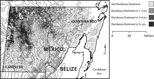
The annual spatial extent of deciduous dominance in the study area ranged from a low of 1709 km² in 2007 to a high of 6366 km² in 2006 (4.7% to 17.5% of forests in the study area). After temporal aggregation into frequency of deciduous dominance classes, 18,875 km² (52%) exhibited deciduous dominance in no years, 11,159 km² (31%) exhibited deciduous dominance in 1–2 years, 3772 km² (10%) exhibited deciduous dominance in 3–4 years, and 2566 km² (7%) exhibited deciduous dominance in 5 or more years (Figure 4). Locations that exhibit frequent deciduous dominance are spatially concentrated in the north-west of the study area, in and along the north-west border of the Calakmul Biosphere Reserve. Although there is no significant local spatial correlation between per-pixel elevation and annual EVI seasonality (r = 0.03), the location of forests that exhibit frequent deciduous dominance relative to regional topography suggests that the local elevational maxima may influence forest behaviour through their effect on weather patterns moving through the region, creating a rain shadow to the west (Figure 4).

Figure 4. Spatial distribution of frequency of deciduousness (years out of 11) map for the study area. Locations of frequent deciduous dominance are concentrated in the northwest of the study area to the immediate northwest of regional uplands.

3.3. Relating climate and deciduousness

Seasonal variability

The seasonal variability regressions, which utilized non-deseasoned vegetation and climate time series, detected relatively strong correspondence between vegetation and precipitation throughout the study area (Table 4).

Table 4. Seasonal variability regression results, for both total-time-series and dry-season-only regressions.

mean-normalized time series dep. Variable: EVI	SEASONAL VARIABILITY				Multivariate Regression (Adj.R ^2)lst0 – precip 012
	Univariate Regressions (R ^2)
	precip 0	precip 1	precip 012	lst0
Total Time Series (N=132)
Total Study Area	0.13	0.19	0.28	0.18	0.34
Never Decid. Dom.	0.11	0.16	0.23	0.12	0.27
1–2 yrs. Decid. Dom.	0.12	0.20	0.29	0.20	0.36
3–4 yrs. Decid. Dom.	0.17	0.26	0.38	0.13	0.50
5– yrs. Decid. Dom.	0.19	0.28	0.42	0.39	0.57
Jan-May Only (N=55)
Total Study Area	0.05	0.11	0.13	0.27	0.33
Never Decid. Dom.	0.05	0.08	0.12	0.20	0.25
1–2 yrs. Decid. Dom.	0.06	0.12	0.14	0.30	0.38
3–4 yrs. Decid. Dom.	0.05	0.15	0.15	0.39	0.47
5– yrs. Decid. Dom.	0.05	0.19	0.15	0.45	0.53
Notes: Variable names are abbreviated: precip0 = same month precipitation; precip1 = 1-month-lagged precipitation; precip012 = total precipitation in same and preceding 2 months; lst0 = same month land surface temperature.

For total-time-series univariate regressions, total precipitation over the same and preceding 2 months was the independent climate variable that correlated most strongly with EVI, followed by 1-month-lagged precipitation, same-month LST and same-month precipitation. For all univariate regressions, model fit is greater (higher R ²) in areas of higher frequency of deciduous dominance than in areas that are rarely or never deciduous dominant. Stronger correspondence in areas of higher deciduous dominance is most pronounced with the same-month LST-independent variable, which explains nearly as much variability of EVI as total precipitation over the same and preceding 2 months in forests that were deciduous dominant in 5 or more years. The Durbin–Watson statistic for the EVI and the same-month LST univariate regression indicated substantial areas of positive residual correlation (d = 1.08, spatial standard deviation = 0.24), but this was the only regression, for any variable over either temporal period, where significant serial correlation was indicated. Maps of per-pixel significance indicate that the relationships between EVI and total precipitation aggregated over the same and preceding 2 months and between EVI and same-month LST were significant (p = 0.001) over nearly the entire study area (98% of study area for both), although the significance of the EVI and same-month LST relationship is likely overestimated because of serial correlation of residuals (Figure 5 ). Spatially averaged over the study area, the adjusted R ² of the multivariate linear regression that explained EVI using total precipitation over the same and preceding 2 months and same-month LST from all months is 0.34, though it is 0.57 in areas that exhibited deciduous dominance in 5 or more years (Figure 6 and Table 4).

Figure 5. ANOVA significance (p = 0.001) of multivariate regressions explaining EVI using same-month temperature and total precipitation in same month and prior 2 months.

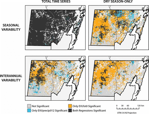
Figure 6. Spatial distribution of adjusted R ² values for multivariate regressions explaining EVI using same-month temperature and total precipitation in same month and prior 2 months. Legend is scaled to the observed maximum and minimum adjusted R ² values.

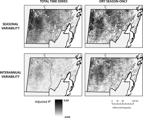
For dry-season-only univariate regressions, same-month LST was the independent climate variable that correlated most strongly with EVI, followed by total precipitation over the same and preceding 2 months, 1-month-lagged precipitation and same-month precipitation. Higher R ² values are associated with areas of higher frequency of deciduous dominance for the univariate regressions involving same-month LST and 1-month-lagged precipitation, but this association is not clear for the regressions involving total precipitation over the same and preceding 2 months and same-month precipitation. Maps of per-pixel significance show that the relationship between EVI and same-month LST is significant (p = 0.001) in 63% of the total study area and in over 90% of forests that exhibited deciduous dominance in 3–4 or in 5 or more years. The relationship between EVI and total precipitation over the same and preceding 2 months was significant in only 26% of the study area, and the spatial extent of significance varied little with frequency of deciduous dominance. Spatially averaged over the study area, the adjusted R ² of the multivariate linear regression that explained EVI using total precipitation over the same and preceding 2 months and same-month LST from dry season months is 0.33 and is 0.53 in areas that exhibited deciduous dominance in 5 or more years.

Interannual variability

The interannual variability regressions, which utilized deseasoned vegetation and climate time series, commonly indicated weaker correlations between deseasoned EVI and deseasoned precipitation and temperature than were observed in the seasonal variability regressions (Table 5).

Table 5. Interannual variability regression results, for both total-time-series and dry-season-only regressions.

deseasoned time seriesdep. Variable: EVI	INTERANNUAL VARIABILITY				Multivariate Regression (Adj.R ^2)std_lst0 – std_precip 012
	Univariate Regressions (R ^2)
	std_precip 0	std_precip 1	std_precip 012	std_lst0
Total Time Series (N=132)
Total Study Area	0.02	0.03	0.05	0.09	0.10
Never Decid. Dom.	0.01	0.02	0.04	0.06	0.07
1–2 yrs. Decid. Dom.	0.02	0.03	0.05	0.10	0.11
3–4 yrs. Decid. Dom.	0.03	0.05	0.08	0.15	0.17
5– yrs. Decid. Dom.	0.04	0.06	0.10	0.18	0.21
Jan-May Only (N=55)
Total Study Area	0.05	0.07	0.10	0.24	0.24
Never Decid. Dom.	0.04	0.06	0.08	0.17	0.17
1–2 yrs. Decid. Dom.	0.05	0.07	0.11	0.27	0.28
3–4 yrs. Decid. Dom.	0.05	0.09	0.14	0.38	0.38
5– yrs. Decid. Dom.	0.06	0.12	0.17	0.40	0.41
Notes: Variable names are abbreviated as in Table 4, with the addition of ‘std_’ to denote that data have been deseasoned.

For total-time-series univariate regressions, same-month LST (deseasoned) was the independent climate variable that correlated most strongly with EVI (deseasoned), while precipitation-derived independent variables (deseasoned) showed weak correlation with EVI (deseasoned). As with the seasonal variability regressions, R ² values are higher in areas of higher frequency of deciduous dominance than in areas that are rarely or never deciduous dominant. The relationship between EVI (deseasoned) and both same-month LST (deseasoned) and total precipitation over the same and preceding 2 months (deseasoned) is significant (p = 0.001) in a smaller portion of the study area (23–45%), but for both independent variables, a high percentage of frequently deciduous dominant areas was significant (56–93%) (Figure 5). A multivariate linear regression that explained EVI (deseasoned) using total precipitation over the same and preceding 2 months (deseasoned) and same-month LST (deseasoned) from all months explained only approximately 10% of the variance in deseasoned EVI over the study area (adjusted R ² of 0.10).

Dry-season-only univariate regressions showed similar patterns to the total-time-series interannual variability regressions, but a much higher correlation between EVI (deseasoned) and same-month LST (deseasoned) were observed (R ² = 0.24 over study area, 0.40 in areas of deciduous dominance in 5 or more years). Relationships between EVI (deseasoned) and precipitation-derived independent variables were weak, but the EVI (deseasoned)/same-month LST (deseasoned) regression was significant in 50% of the study area and in over 90% of forests in the highest two frequency of deciduous dominance classes (Figure 5). A multivariate linear regression that explained EVI (deseasoned) using total precipitation over the same and preceding 2 months (deseasoned) and same-month LST (deseasoned) from dry season months showed little improvement in explanatory power relative to the univariate regression involving same-month LST (deseasoned).

4. Discussion

Temporal profiles of EVI, TRMM precipitation and MODIS LST averaged over the total study area display a clear seasonal pattern. Substantially less interannual variability is observed for annual maximum EVI than for annual minimum EVI, supporting the use of annual maximum EVI to normalize the metric used to indicate deciduous dominance. LST displays a distinct seasonal temporal pattern (highs in dry season, lows in wet season) with little interannual variability. Although precipitation also displays a seasonal temporal pattern, the magnitude of precipitation in a given month varies widely from year to year. Profiles for both the deciduous and non-deciduous forest target locations show a similar seasonal pattern for precipitation and temperature, but the differences in EVI over time are striking. As expected, the range of observed EVI in the non-deciduous forest is relatively small, and seasonal cycles are difficult to distinguish. In contrast, minimum annual EVI in the deciduous forest typically occurs in April or May and is a value approximately half of annual maximum EVI. This pattern indicates that deciduous and non-deciduous forests experience similar seasonal patterns of environmental conditions, but the spatial variability in the seasonal range of EVI is due to varying levels of vegetation sensitivity to relatively warm or dry conditions, on the order of approximately 2°C and 100 mm/year for temperature and precipitation, respectively (Figure 3; Lawrence 2005; Schmook et al. 2011).

Deciduous dominance was not observed in over half of the study area and was observed in 5 or more years in less than a tenth of the study area. The locations in which deciduousness is a spatially dominant, vegetative response are concentrated in the north-west of the study area. These locations are slightly warmer and drier than forests in the east, closer to the Caribbean Sea. Frequent deciduous dominance shows a spatial relationship to regional topography, with frequently deciduous forests concentrated in areas with west/north-west aspect (Figure 4). Weather systems typically move from east to west in the southern Yucatán, and the area of concentrated deciduous dominance falls in a topographic rain shadow that may not be adequately captured by the spatially coarse precipitation data (˜28 × 28 km). Use of the Frequency of Deciduous Dominance map to extract regression statistics indicates the specific climate–vegetation relationships associated with deciduousness.

The difference in R ² values between the total-time-series and dry-season-only sets of seasonal variability regressions suggest that the environmental conditions that govern overall vegetation phenology are different from those that directly influence dry season deciduousness. For the total-time-series seasonal variability regressions, total precipitation over the same and preceding 2 months is seen to be the most significant independent variable as a predictor of EVI, and the observed significance of same-month LST is likely to be inflated by serial correlation of residuals. The observed strong relationship between total precipitation over the same and preceding 2 months and EVI comports with the findings of Whigham et al. (1990) and the expectations of Lawrence (2005). In contrast to the relative strength of independent climate variables observed in total-time-series regressions, for dry-season-only seasonal variability regressions, same-month LST clearly explains EVI better than total precipitation over the same and preceding 2 months, and the difference in performance is greater in forests that typically exhibit deciduousness. The association between dry-season EVI and dry-season precipitation is no stronger in deciduous forest than in non-deciduous forest, a finding that has likely implications for the effect of deciduous litter on forest fires in the region, the number and size of which is observed to correlate strongly with dry-season precipitation.

Both the total-time-series and dry-season-only interannual variability regressions indicate that atypically low EVI (deseasoned) is more strongly explained by atypically high same-month LST (deseasoned) than by atypically low total precipitation over the same and preceding 2 months (deseasoned) (Figure 6). The absolute difference in explanatory power does differ substantially between the total-time-series and dry-season-only regressions, with dry-season-only same-month LST (deseasoned) explaining an average of 24% of EVI (deseasoned) variability in the study area and around 40% of EVI (deseasoned) variability in forests that were frequently deciduous.

5. Conclusion

This study mapped the phenomenon of deciduousness in the southern Yucatán and described the typical environmental conditions in which it is observed. Areas of deciduous dominance are characterized by warmer temperatures (˜2°C) and lower precipitation (˜100 mm/year) than those seen in non-deciduous forests, and the areas of the most frequent deciduous dominance appear to be concentrated in a regional rain shadow. In regressions on seasonal data, accumulated precipitation over the same and preceding 2 months is more closely tied to the full-year phenological cycle of vegetation, whereas temperature is a stronger determinant of the intensity of dry season deciduousness. The effect of higher temperatures on water potential difference and potential evaporation is not specific to the study area, and future studies of deciduousness should examine the phenomenon in relation to this environmental variable. Additionally, regressions on interannual variability indicate that vegetative vigour is sensitive at all times to atypically high temperature, but that this sensitivity is heightened during the dry season months.

Future research into dry season deciduousness in the region should examine deciduousness at finer spatial scales to further constrain the conditions with which the phenomenon coincides and to more clearly demonstrate the mechanisms driving deciduousness. Finer temporal scale data series could also be leveraged to examine the impact of environmental conditions on the timing of phenological events. Finally, exploration of the roles of forest age and past land use in complementing or compounding the influence of environmental conditions in prompting deciduousness has the potential to account for additional variability in deciduousness that is not explained by environmental conditions alone.

Acknowledgements

This research was supported by the Gordon and Betty Moore Foundation under Grant No. 1697. The authors thank the staff of Clark Labs, Worcester (MA), for facilitating this work using Idrisi® software.

References

- Anderson , L. O. , Aragão , L. , Shimabukuro , Y. E. , Almeida , S. and Huete , A. 2011 . Use of Fraction Images for Monitoring Intra-Annual Phenology of Different Vegetation Physiognomies in Amazonia.” . International Journal of Remote Sensing , 32 : 387 – 408 .
- Bohlman , S. A. 2010 . Landscape Patterns and Environmental Controls of Deciduousness in Forests of Central Panama.” . Global Ecology and Biogeography , 19 : 376 – 385 .
- Borchert , R. 1994 . Soil and Stem Water Storage Determine Phenology and Distribution of Tropical Dry Forest Trees.” . Ecology , 75 : 1437 – 1449 .
- Borchert , R. 1999 . Climatic Periodicity, Phenology, and Cambium Activity in Tropical Dry Forest Trees.” . IAWA Journal , 20 : 39 – 247 .
- Ceballos , G. and Brown , J. H. 1995 . Global Patterns of Mamalian Diversity, Endemism, and Endangerment.” . Conservation Biology , 9 : 559 – 568 .
- Chapin , F. S. , Matson , P. A. and Mooney , H. A. 2002 . Principles of Terrestrial Ecosystem Ecology , 544 New York , NY : Springer-Verlag .
- Christman , Z. , Rogan , J. , Schneider , L. , Schmook , B. , Lawrence , D. , Bumbarger , N , Cuba , N. , Millones , M. , Zager , I. and II Turner , B. L. Mapping intra-annual phenological patterns of deciduous leaf drop in the semi-dry tropical forests of the Mexican Yucatán Peninsula using Landsat ETM – forthcoming
- Condit , R. , Aguilar , S. , Hernandez , A. , Perez , R. , Lao , S. , Angehr , G. , Hubbell , S. P. and Foster , R. B. 2004 . Tropical Forest Dynamics Across a Rainfall Gradient and the Impact of an El Niño Dry Season.” . Journal of Tropical Ecology , 20 : 51 – 72 .
- Condit , R. , Watts , K. , Bohlman , S. , Pérez , R. , Foster , R. B. and Hubbell , S. P. 2000 . Quantifying the Deciduousness of Tropical Forest Canopies Under Varying Climates.” . Journal of Vegetation Science , 11 : 649 – 658 .
- De Beurs , K. M. and Henebry , G. M. 2010 . “ Spatio-Temporal Statistical Methods for Modeling Land Surface Phenology.” . In Phenological Research: Methods for Environmental and Climate Change Analysis , Edited by: Hudson , I. L. and Keatley , M. R. 177 – 208 . Dordrecht : Springer .
- Durbin , J. and Watson , G. S. 1951 . Testing for Serial Correlation in Least Squares Regression: II.” . Biometrica , 38 : 159 – 178 .
- Farr , T. G. , Rosen , P. A. , Caro , E. , Crippen , R. , Durren , R. , Hensley , S. and Kobrick , M. 2007 . The Shuttle Radar Topography Mission.” . Reviews of Geophysics , 45 : 33
- Foody , G. M. 2002 . Hard and Soft Classifications by a Neural Network with a Non-Exhaustively Defined Set of Classes.” . International Journal of Remote Sensing , 23 ( 18 ) : 3853 – 3864 .
- Hartshorn , G. S. 1988 . “ Tropical and Subtropical Vegetation of Meso-America.” . In North American Terrestrial Vegetation , Edited by: Barbour , M. and Billings , W. 365 – 390 . New York : Cambridge University Press .
- Hernandez , P. A. , Franke , I. , Herzog , S. K. , Pacheco , V. , Paniagua , L. , Quintana , H. L. and Soto , A. 2008 . Predicting Species Distributions in Poorly Studied Landscapes.” . Biodiversity Conservation , 17 : 1353 – 1366 .
- Holbrook , N. M. , Whitbeck , J. L. and Mooney , H. A. 1995 . “ Drought Responses of Neotropical Dry Forest Trees.” . In Seasonally Dry Tropical Forests , Edited by: Bullock , S. , Mooney , H. and Medina , E. 243 – 276 . New York : Cambridge University Press .
- Huete , A. R. , Didan , K. , Miura , T. , Rodriguez , E. P. , Gao , X. and Ferreira , L. G. 2002 . Overview of the Radiometric and Biophysical Performance of the MODIS Vegetation Indices.” . Remote Sensing of Environment , 83 : 195 – 213 .
- Huffman , G. , Adler , R. , Yang , H. D. , Guojun , G. , Bowman , K. P. and Stocker , E. F. 2007 . The TRMM Multisatellite Precipitation Analysis (TMPA): Quasi-Global, Multiyear, Combined-Sensor Precipitation Estimates at Fine Scales.” . Journal of Hydrometeorology , 8 : 38 – 55 .
- Hwang , T. , Song , C. , Vose , J. M. and Band , L. E. 2011 . Topography-Mediated Controls on Local Vegetation Phenology Estimated From MODIS Vegetation Index.” . Landscape Ecology , 26 ( 4 ) : 37 – 50 .
- Immerzeel , W. W. , Rutten , M. M. and Droogers , P. 2009 . Spatial Downscaling of TRMM Precipitation Using Vegetative Response on the Iberian Peninsula.” . Remote Sensing of Environment , 113 : 362 – 370 .
- Ito , E. , Araki , M. , Tith , B. , Pol , S. , Trotter , C. , Kanzaki , M. and Ohta , S. 2008 . Leaf-Shedding Phenology in Lowland Tropical Seasonal Forests of Cambodia as Estimated From NOAA Satellite Images.” . IEEE Transactions on Geoscience and Remote Sensing , 46 : 2867 – 2871 .
- Janzen , D. H. 1988 . “ Tropical Dry Forests: The Most Endangered Major Tropical Ecosystem.” . In Biodiversity , Edited by: Wilson , E. O. 130 – 137 . Washington , DC : National Academy Press .
- Justice , C. O. , Vermote , E. , Townshend , J. R. , Defries , R. , Roy , D. P. , Hall , D. K. and Salamonson , V. V. 1998 . The Moderate Resolution Imaging Spectroradiometer (MODIS): Land Remote Sensing for Global Change Research.” . IEEE Transactions on Geoscience and Remote Sensing , 36 ( 4 ) : 1228 – 1249 .
- Kauth , R. J. and Thomas , G. S. 1976 . “ The Tasseled Cap-A Graphic Description of the Spectral-Temporal Development of Agricultural Crops as Seen by Landsat ” . In Proceedings of the the Symposium on Machine Processing of Remotely Sensed Data , Edited by: Wilson , E. O. 4B41 – 4B50 . West Lafayette : Purdue University .
- Lawrence , D. 2005 . Regional-Scale Variation in Litter Production and Seasonality in Tropical Dry Forests of Southern Mexico.” . Biotropica , 37 ( 4 ) : 561 – 570 .
- Márdero , J. and Silvia , S. 1995 . ECOSUR. Tesis: “Sequías y efectos en las prácticas agrícolas en familias campesinas del Sur de la Península de Yucatán” [Effects of Drought on Agricultural Practices of Rural Families in the Southern Yucatán Peninsula] , 1 – 9 . Director y asesor(es) : Birgit Inge Schmook (Director), Guadalupe del Carmen Alvarez Gordillo (Asesor) .
- Morisette , J. T. , Richardson , A. D. , Knapp , A. K. , Fisher , J. I. , Graham , E. A. , Abatzoglou , J. and Wilson , B. E. Tracking the Rhythm of the Seasons in the Face of Global Change: Phenological Research in the Twenty-First Century.” . Frontiers in Ecology and the Environment , 7 253 – 260 .
- Murphy , P. G. and Lugo , A. E. 1995 . “ Dry Forests of Central America and the Caribbean.” . In Seasonally Dry Tropical Forests , Edited by: Bullock , S. , Mooney , H. and Medina , E. 9 – 34 . New York : Cambridge University Press .
- Murphy , P. G. and Lugo , A. E. 1986 . Ecology of Tropical Dry Forest.” . Annual Review of Ecology and Systematics , 17 : 67 – 88 .
- Myers , N. 1984 . The Primary Source: Tropical Forests and Our Future , 484 New York : W.W. Norton .
- Nepstad , D. C. , Jipp , P. , Moutinho , P. , Negreiros , G. and Vieira , G. 1995 . “ Forest Recovery Following Pasture Abandonment in Amazoˆnia: Canopy Seasonality, fire Resistance and Ants.” . In Evaluating and Monitoring the Health of Large-Scale Ecosystems , Edited by: Rapport , D. , Caudet , C. L. and Calow , P. 333 – 349 . Berlin : Springer .
- Nicholson , S. E. and Entekhabi , D. 1987 . Rainfall Variability in Equatorial and Southern Africa: Relationship with Sea-Surface Temperature Along the Southwest Coast of Africa.” . Journal of Applied Meteorology and Climatology , 26 : 561 – 578 .
- Park , S. 2010 . A Dynamic Relationship Between the Leaf Phenology and Rainfall Regimes of Hawaiian Tropical Ecosystems: A Remote Sensing Approach.” . Singapore Journal of Tropical Geography , 31 : 371 – 383 .
- Pennington , R. T. , Prado , D. E. and Pendry , C. A. 2000 . Neotropical Seasonally Dry Forests andQuaternary Vegetation Changes.” . Journal of Biogeography , 27 : 261 – 273 .
- Pérez-Salicrup , D . 2004 . “ Forest Types and Their Implications,.” . In Integrated Land-Change Science and Tropical Deforestation in the Southern Yucatán: Final Frontiers , Edited by: Turner , B. L. , Geoghegan , J. and Foster , D. 63 – 80 . Oxford : Oxford University Press .
- Querejeta , J. I. , Estrada-Medina , H. , Allen , M. F. and Jimenez-Osornio , J. J. 2007 . Water Source Partitioning Among Trees Growing on Shallow Karst Soils in a Seasonally Dry Tropical Climate.” . Oecologia , 152 : 26 – 36 .
- Reyna-Hurtado , R. , Rojas-Flores , E. and Tanner , G. W. 2009 . Home Range and Habitat Preferences of White-Lipped Peccaries (Tayassu Pecari) in Calakmul, Campeche, Mexico.” . Journal of Mammalogy , 90 ( 3 ) : 1199 – 1209 .
- Richardson , A. D. , Jenkins , J. P. , Braswell , B. H. , Hollinger , D. Y. , Ollinger , S. and Smith , M. L. 2007 . Use of Digital Webcam Images to Track Spring Green-up in a Deciduous Broadleaf Forest.” . Oecologia , 152 : 323 – 334 .
- Rueda , X. 2010 . Understanding Deforestation in the Southern Yucatán: Insights From a Sub-Regional, Multi-Temporal Analysis.” . Regional Environmental Change , 10 : 175 – 189 .
- Schaaf , C. B. , Gao , F. , Strahler , A. H. , Lucht , W. , Li , X. , Tsang , T. and Strugnell , N. C. 2002 . First Operational BRDF, Albedo Nadir Reflectance Products From MODIS.” . Remote Sensing of Environment , 83 : 135 – 148 .
- Schmook , B. , Dickson , R. P. , Sangermano , F. , Vadjunic , J. M. , Eastman , J. R. and Rogan , J. 2011 . A Step-Wise Land-Cover Classification of the Tropical Forests of the Southern Yucatán, Mexico.” . International Journal of Remote Sensing , 32 ( 4 ) : 1139 – 1164 .
- Skole , D. and Tucker , C. 1993 . Tropical Deforestation and Habitat Fragmentation in the Amazon: Satellite Data From 1978 to 1988.” . Science , 260 : 1905 – 1910 .
- Swain , S. , Wardlow , B. D. , Narumalani , S. , Tadesse , T. and Callahan , K. 2011 . Assessment of Vegetation Response to Drought in Nebraska Using Terra-MODIS Land Surface Temperature and Normalized Difference Vegetation Index.” . GIScience & Remote Sensing , 48 : 432 – 455 .
- Tateishi , R. and Ebata , M. 2004 . Analysis of Phenological Change Patterns Using 1982–2000 Advanced Very High Resolution Radiometer (AVHRR) Data.” . International Journal of Remote Sensing , 25 : 2287 – 2300 .
- Trejo , I. and Dirzo , R. 2000 . Deforestation of Seasonally Dry Tropical Forest: A National and Local Analysis in Mexico.” . Biological Conservation , 94 ( 2 ) : 133 – 142 .
- Turner , B. L. , Geoghegan , J. and Foster , D. 2004 . Integrated Land-Change Science andTropical Deforestation in the Southern Yucatán , 348 Oxford : Oxford University Press .
- Ustin , S. L. , ed. 2004 . Remote Sensing for Natural Resource Management and Environmental Monitoring , 768 New York : John Wiley & Sons .
- Valenzuela , D. and Ceballos , G. 2000 . Habitat Selection, Home Range, and Activity of the White-Nosed Coati (Nasua Narica) in a Mexican Tropical Dry Forest.” . Journal of Mammalogy , 81 : 810 – 819 .
- Vester , H. , Lawrence , D. , Eastman , J. R. , Turner , B. L. , Calmé , S. , Dickson , R. , Pozo , C. and Sangermano , F. 2007 . Land Change in the Southern Yucatán and Calakmul Biosphere Reserve: Effects on Habitat and Biodiversity.” . Ecological Applications , 17 ( 4 ) : 989 – 1003 .
- Vincent , R. K. , Qin , X. , McKay , R. M. L. , Miner , J. , Czajkowski , K. , Savino , J. and Bridgeman , T. 2004 . Phycocyanin Detection From LANDSAT TM Data for Mapping Cyanobacterial Blooms in Lake Erie.” . Remote Sensing of Environment , 89 : 381 – 392 .
- Vitousek , P. M. and Sanford , R. L. 1986 . Nutrient Cycling in Moist Tropical Forest.” . Annual Review of Ecological Systems , 17 : 137 – 167 .
- Wan , Z. and Li , Z. -L. 1997 . A Physics-Based Algorithm for Retrieving Land-Surface Emissivity and Temperature From EOS/MODIS Data.” . IEEE Transactions on Geoscience and Remote Sensing , 35 : 980 – 996 .
- Wan , Z. , Zhang , Y. , Zhang , Q. and Li , Z. L. 2004 . Quality Assessment and Validation of the MODIS Global Land Surface Temperature.” . International Journal of Remote Sensing , 25 ( 1 ) : 261 – 274 .
- Wang , J. , Price , K. P. and Rich , P. M. 2001 . Spatial Patterns of NDVI in Response to Precipitation and Temperature in the Central Great Plains.” . International Journal of Remote Sensing , 22 ( 18 ) : 3827 – 3844 .
- Whigham , D. F. , Zugasty Towle , P. , Cabrera Cano , E. , O'Neill , K. and Ley , E. 1990 . The Effect of Annual Variation in Precipitation on Growth and Litter Production in a Tropical Dry Forest in the Yucatán of México.” . Tropical Ecology , 31 : 23 – 34 .
- White , M. A. and Nemani , R. R. 2006 . Real-Time Monitoring and Short-Term Forecasting of Land Surface Phenology.” . Remote Sensing of Environment , 104 : 43 – 49 .
- Xiao , X. , Hagen , S. , Zhang , Q. , Keller , M. and Moore , B. 2006 . Detecting Leaf Phenology of Seasonally Moist Tropical Forests in South America with Multi-Temporal MODIS Images.” . Remote Sensing of Environment , 103 ( 4 ) : 465 – 473 .
- Zhang , X. , Friedl , M. A. , Schaaf , C. B. , Strahler , A. H. and Liu , Z. 2005 . Monitoring the Response of Vegetation Phenology to Precipitation in Africa by Coupling MODIS and TRMM Instruments . Journal of Geophysical Research , 110 : D12103 doi: 10.1029/2004JD005263