Monitoring fugitive dust emission sources arising from construction: a remote-sensing approach

Abstract

Construction-related soil disturbance (e.g., road construction, trenching, land stripping, earthmoving, and blasting) is a significant source of fugitive (airborne) dust in the atmosphere. Fugitive dust is a primary cause of decreased air quality and may carry airborne pathogens. We use Landsat Thematic Mapper (TM) remote-sensing data spanning 1994 through 2009 over southern Arizona to identify source areas of construction-related activity likely to produce fugitive dust. We correlate temporal changes in the mid-infrared spectral response to dust sources from local construction. Image differencing of the TM band 5 (mid-infrared), with a change threshold of ±5 SD of the mean, suitably estimates the location and area affected by construction-related soil disturbance. Estimated dust-producing surface area ranges from 10.0 (1996–1997) to 28.3 km² (2004–2005), or 0.16–0.44% of the Pima County study area. Our methods aim to automate monitoring of fugitive dust sources by environmental and health agencies and to provide inputs to dust transport, air quality, and climate models.

Keywords:

• soil disturbance
• construction
• fugitive dust
• Valley Fever
• remote sensing
• Landsat
• image differencing

1. Introduction and background

1.1. Introduction

Dust can be defined as “small solid particles, conventionally taken as those particles below 75 µm in diameter, which settle out under their own weight but which may remain suspended for some time” (ISO 1994). Dust is termed fugitive when it is not discharged to the atmosphere in a confined flow stream, not collected by a capture system, or not emitted from a stack, chimney, or tailpipe (EPA 1995). Common sources of fugitive dust include unpaved roads, bare ground, agricultural tilling, storage piles, and construction-related soil disturbance (Watson et al. 2002; Chow et al. 2003; Ho et al. 2003; Samara 2005).

We aim here to define space–time variations in fugitive dust, its health and environmental consequences, and its regulatory framework. We explore remote-sensing technology to assess fugitive dust sources, introducing a change detection model to identify potential sources. Collateral dust inspection data and geographical information system (GIS) methods validate this model.

1.2. Health and environmental consequences of fugitive dust

Particles less than 10 µm are inhaled readily into the lungs where they may accumulate, react, be absorbed, or be cleared. Scientific studies (EPA 2003) have linked particle pollution with a series of significant health problems, including irritation of the airways, coughing, decreased lung function, aggravated asthma, chronic bronchitis, and premature death in people with heart or lung disease. Ecologists and environmental scientists often overlook the importance of dust- and wind-driven processes, yet these processes exert a fundamental influence on biogeochemical and ecological systems (Field et al. 2010).

As of 30 August 2011, EPA identified over 38 National Ambient Air Quality Standard (NAAQS) nonattainment areas in the United States for PM₁₀ (particulate matter less than 10 µm), and these areas affect 39 counties with a population of over 25 million (EPA 2012c). Large populations may therefore be exposed to unhealthy air, which in some cases is known to carry disease pathogens.

1.3. Coccidioidomycosis: a disease produced by the inhalation of airborne pathogens

Coccidioidomycosis (Valley Fever) is a systemic infection caused by inhalation of airborne spores from Coccidioides spp., which are fungi found in the soil in the southwestern United States, including Arizona and California, and parts of Mexico (Galgiani 1999). Coccidioidomycosis has increased epidemically in Arizona within the last decade (Park et al. 2005). The saprophytic phase of the species exists as slender filaments of cells that grow in the upper part of the soil (Kolivras et al. 2001).

Infection occurs typically following disturbance activities or natural events that disrupt the surface soil. This results in aerosolization of the fungal arthrospores and a subsequent spore source for inhalation by a host (Elconin, Egeberg, and Egeberg 1964; Maddy 1957; Schneider et al. 1997; Swatek 1970). There is a remarkable association of disease cases with previous exposures to dust storms, archeological digs, and occupational exposure to agricultural and construction dust (Emmons 1942; Kirkland and Fierer 1996; Pappagianis and Einstien 1978; Werner 1974). The mechanisms of the association are not established. We look now at the origins of fugitive dust as a vehicle for pathogen dispersal.

1.4. Soil disturbance and construction-generated fugitive dust

A disturbed surface area is any portion of land that has been moved physically, uncovered, destabilized, or otherwise modified from its natural condition, thereby increasing the potential for fugitive dust emissions (EPA 2012a). The dust-generation process during surface disturbance is caused by two basic physical phenomena: (1) pulverization and abrasion of surface materials by application of mechanical force through implements (wheels, blades, etc.) and (2) entrainment of dust particles by the action of turbulent air currents, such as wind erosion of an exposed surface by wind speeds over 19 km/h (EPA 1995).

Heavy construction, such as building and road construction, consists of a series of operations, for example, land clearing, frilling and blasting, ground excavation, earth moving, and structural construction (EPA 1995). Each phase of the cycle exhibits its own duration and potential for dust generation. Furthermore, tracked out material on adjacent roadways can be suspended by traffic, and high-wind events can lead to emissions from cleared land and material stockpiles.

1.5. Assessing the spatial and temporal distribution of fugitive dust sources

Fugitive dust sources arising from construction may be underestimated in typical assessments and modeling. Previous studies for fugitive dust sources focused mainly on paved or unpaved road dust, soil dust and cement; source profiles for construction dust are limited (Kong et al. 2011).

Strategies for assessing and monitoring fugitive dust source areas include field surveys, collection of dust samples using various methods, census and statistical methods, and modeling of atmospheric circulation patterns (Stefanov, Ramsey, and Christensen 2003). The multistage construction cycle also generates changes in spectral properties as the surface is modified (Jensen and Toll 1982), which may be detected by remote-sensing methods.

1.6. Remote sensing to detect change in surface spectral properties

Remote sensing, a source of multispectral data, can provide fundamental, new scientific information, including land-cover change. The basic premise in using remote-sensing data for change detection is that changes in land cover must result in changes in radiance values, and these changes must be large with respect to radiance changes caused by other factors such as atmospheric conditions, sun angle, and soil moisture (Ingram, Knapp, and Robinson 1981). Selecting the appropriate data and change detection technique according to the nature of the problem under investigation is critical in any change detection study (Jensen and Im 2007).

Image differencing is the most widely applied algorithm for change detection (Coppin et al. 2004). Image differencing is the subtraction of spatially coregistered images collected at different times, producing a “change” image (Jensen 2005). Image subtraction produces positive and negative values in areas of radiance change, and values of zero in areas of no change. In an 8-bit remote-sensing system (where pixel values range from 0 to 255), the potential range of difference values is −255 to +255. Identifying appropriate spectral thresholds that discriminate “change” pixels from “no-change” pixels enables generation of a binary change image.

1.7. Image differencing to detect change at the urban fringe

Image differencing is known to provide superior results for identifying change due to natural or rural area conversion to urban land (Fung 1990; Jensen and Toll 1982; Ridd and Liu 1998; Royal 1980; Toll, Royal, and Davis 1980). This success is attributed partly to enhancement of contrast between vegetated and nonvegetated surfaces due to chlorophyll absorption, such as in the red portion of the spectrum.

None of the spectral band selection algorithms analyzed in these studies was found to be clearly superior; according to the authors, the choice depends on specific environmental conditions in play and application objectives (Ridd and Liu 1998). The Landsat Thematic Mapper 5 (TM), which was not available for the earlier studies, provides data since 1984 in seven spectral regions, including the middle infrared (MIR), at 30-m spatial resolution (NASA 2012b).

1.8. Mid-infrared spectral region for surface change detection

The MIR spectral region is known to discriminate moisture content of soil and vegetation, and it is used often in drought and plant vigor studies (Howarth and Wickware 1981; Maki, Ishiahra, and Tamura 2004; NASA 2012a; USGS 2010). The TM MIR bands 5 and 7, in one study, accounted for much of the separability between wetland land-cover types during image classification (Jensen et al. 1993). The authors also applied change/no-change masks generated from TM band 5 (1.55–1.75 µm) difference images of upland, nontidal areas to improve classification accuracy.

Generic spectral reflectance profiles suggest that soil, vegetation, and water are well-distinguished in the MIR region, whereas spectral confusion can occur in other spectral regions. We compiled a list of soil and vegetation spectral indices which use the MIR spectral region (Table 1). We focus on the Landsat MIR for dust source detection studies in southern Arizona.

Table 1. Spectral indices emphasizing soil and vegetation moisture properties using Landsat TM.

Index	Formula	Reference
Bare soil index (BI)	[(SWIR + R) – (NIR + B)]/ [(SWIR + R) + (NIR + B)]	Roy, Miyatake, and Rikimaru (1997)
	(B5+B3) − (B4+B1)/(B5 + B3) + (B4 + B1)	Chen et al. (2004)
Normalized difference soil index (NDSI)	[SWIR – NIR]/[SWIR + NIR]	Rogers and Kearny (2004)
	B5 − B4/B5+B4
Normalized difference built-up index (NDBI)	[SWIR – NIR]/[SWIR + NIR]	Zha, Ga, and Ni (2003)
	B5 − B4/B5 + B4
BU or built-up areas	NDBI − NDVI	He et al. (2010)
Normalized difference bareness index (NDBaI)	[SWIR – TIR]/[SWIR + TIR]	Zhao and Chen (2005)
	B5 − B6/B5 + B6
Normalized difference water index (NDWI)	[G – NIR]/[ G + NIR]	McFeeters (1996)
	B2 − B4/B2 + B4
Normalized difference water index (NDWI)	[R – SWIR]/[R + SWIR]	Rogers and Kearny (2004)
	B3 − B5/B3 + B5
Normalized difference water index (NDWI)	[NIR – SWIR]/[NIR + SWIR] B4 − B5/B4 + B5	Gao (1996)Jackson et al. (2004)
Normalized difference moisture index (NDMI)	[NIR – SWIR]/[NIR + SWIR] B4 − B5/B4 + B5	Wilson and Sader (2002)
Normalized difference infrared index (NDII)	[NIR – SWIR]/[NIR + SWIR] B4 − B5/B4 + B5	Hardisky, Smart, and Klemas (1983)
Note: Spectral regions and the corresponding Landsat TM bands are shown in the Formula block.

1.9. Southern Arizona study area

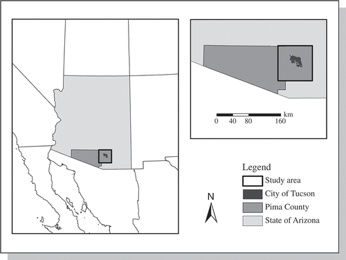
Our study area lies within the eastern portion of Pima County, Arizona, and consists of approximately 13,000 km² in area (Figure 1). Pima County is located in the southwestern region of the United States and in the southern portion of Arizona. It shares approximately 200 km of border with the state of Sonora, Mexico. The population of Pima County is 980,263 (Census 2012). The vast majority of the county population lies in and around the city of Tucson (518,956; 2006), which fills up much of the eastern part of the county. Tucson is Arizona's second largest city, and it is a major commercial and academic center. A ring of communities, unincorporated urban development, and undeveloped areas surround the city. The western half of the county is sparsely populated, and it is not included in the study area.

Figure 1. Study area map including southwestern United States, northwestern Mexico, the state of Arizona, Pima County and the city of Tucson.

The Tucson region is a desert valley surrounded by five mountain ranges. The study area lies within the Sonoran Desert, which is a lush desert with legume trees and columnar cacti as dominant flora. Thousands of acres of the Sonoran Desert have been bladed for the construction of houses and commercial strip malls (AIA 2007). Between 1980 and 1990, the city's area increased by over 50% through the annexation of unincorporated land, and currently, the total area encompassed within the city limits is 585 km². As the city has expanded, so too has development in the immediate “fringe” areas.

2. Data and methods

2.1. Image preprocessing

Landsat Thematic Mapper 5 (TM) archive images are processed to the Level 1 Product Generation System with precision and terrain correction (LPGS, L1T), and with cubic convolution resampling (USGS 2011). The eastern Pima County, AZ, study area is located in Path 36 and Row 38 of the Landsat Worldwide Reference System. To minimize annual phenological effects, we selected Landsat 5 TM MIR images captured in May or June for each year of the study period (1984–2009). Comparisons of random points within the area of interest showed good spatial registration to within one pixel between the images, and therefore additional fine-tuning beyond USGS processing was not required.

We incorporated updated radiometric calibration coefficients specific to the new USGS Landsat open-access archive (Chander, Markham, and Helder 2009) to achieve conversion of calibrated digital numbers to absolute units of at-sensor spectral radiance. We converted each image to atmospheric-corrected surface reflectance using the cosine approximation model (COST; Chavez 1996). The COST model implements an improved dark-object atmospheric correction for Landsat TM multispectral data (bands 1–5 and 7).

2.2. Air quality dust inspection data

The Pima County Department of Environmental Quality (PDEQ) requires entities or individuals conducting land stripping or earthmoving in excess of one acre, trenching in excess of 300 feet, road construction in excess of 50 feet, and blasting to obtain an air quality activity permit through the PDEQ (Pima 2012). In addition, the PDEQ operates an inspection program to monitor and regulate soil-disturbance activities likely to generate fugitive dust. The dust inspections are initiated by complaints from the public, referrals from other public agencies, and data obtained from the county's fugitive dust-generating activity permit program.

As of December 2002, PDEQ inspectors document geographic coordinates for all PDEQ inspections using hand-held Global Positioning System (GPS) devices. More than 90% of permits received by the department are inspected, and each permit is usually inspected more than once to assess progress of the specific activity. The number of repeat inspections is determined by the respective activity's duration and scope (Pima 2012).

We obtained data for PDEQ fugitive dust-generating activity inspections occurring between January 2003 and January 2006 by public information request. Spatial coordinates for each inspection point were subsetted into annual periods beginning in June and ending in May to match the satellite annual change detection image dates. The data were entered in a GIS and used to develop and validate the remote-sensing method.

2.3. Single-band image subtraction for change detection

We explored several techniques to ascertain change likely to be associated with soil disturbance. Based on simplicity, its association with soil properties and vegetation moisture (USGS 2010; Table 1), and superior comparisons with the PDEQ dust inspection data set (see Section 4.2), we selected single-band differencing of the TM band 5 to perform our study.

Full-scene TM band 5 images were subtracted from the succeeding year's image to generate successive annual change images that cover the 15-year span of the study (1994–2009). Each change image was subsetted to the approximately 640 km² study area. A mask was applied to remove areas in excess of 1000 m elevation (generally the regional mountain ranges) in order to focus on the region's urban areas and their periphery. An additional mask derived the USGS Regional Southwest Gap Project (SWReGAP 2004) was applied to remove agricultural and mining land cover in the northwest corner and south-center areas of the study area (10% of the remaining study area) to focus on construction-related activity.

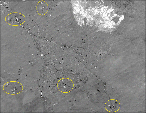
Figure 2 displays a TM band 5 difference image of eastern Pima County for 2003–2004. Areas of greatest change are indicated by pixels with increased brightness (white) or increased darkness (black). Change resulting from anthropogenic disturbance is often identified in these images as having non-natural patterns, such as straight lines and rectangles, as highlighted by circles in the image.

Figure 2. A change detection image of the Tucson, AZ, metropolitan region between May 2003 and June 2004 using band differencing in the MIR spectral region (Landsat TM band 5). Change of interest to this study is noted as the bright or dark polygons throughout the image including the circled areas. This change is attributed primarily to human disturbance such as subdivision home construction. The large, bright area at the top (north) edge of the scene results from change induced by the Aspen fire occurring in the Santa Catalina Mountains during the summer of 2003. A mask was applied to remove areas in excess of 1000 m elevation, thus the fire scar area was not included in the study.

2.4. Geographic information system analysis

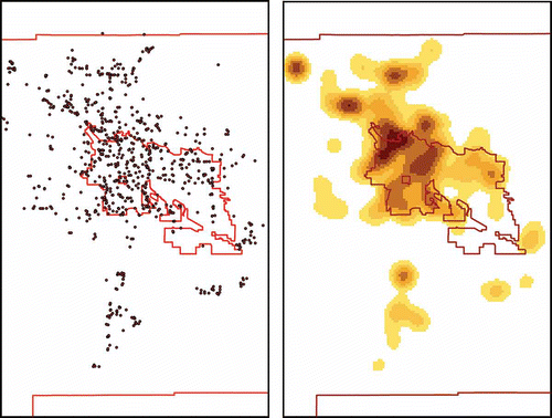
We added the PDEQ dust inspection coordinates, subsetted to match the temporal periods of the satellite change images, into a GIS layer (ESRI ArcMap 9.2 and 9.3), and converted them to shape files. We applied a kernel density function to each set using consistent default input parameters, including a search radius (4670 m) and an output grid cell size (0.220 km²). The kernel density function, based on Silverman (1986), fits a surface over each point, with the surface value being highest at the location of the point and diminishes to zero at the search radius. The density at each output raster cell is calculated by adding the values of all the kernel surfaces where they overlay the raster cell center. Figure 3 displays the dust inspection data points and their corresponding kernel density plot for the 2004–2005 annual period.

Figure 3. Spatial coordinates for fugitive dust inspections performed by the Pima County Department of Environmental Quality to assess construction-related activity between June 2004 and May 2005 are obtained and entered into a GIS (left). A kernel density function is applied to generate a density plot (right). A search radius of 4.67 km and an output cell (grid) size of 0.220 km² are used. Tucson City limits and the Pima County border are also shown.

We overlaid the satellite change images by their corresponding kernel density plot of dust inspection points. We are interested in the extent to which areas with high change detection signal (increased bright or dark pixels) are spatially consistent with areas showing high dust inspection density (reddish or darkish hue). The 2003–2004 comparison is displayed in Figure 4. Qualitative comparisons reveal good agreement between the PDEQ dust inspection and the remote-sensing change detection data sets. We developed a thresholding strategy to limit false positives derived from these change detection protocols.

Figure 4. Remote-sensing-derived change image with the Pima County DEQ dust inspection point kernel density overlay for the Tucson, AZ, metropolitan area between May 2003 and June 2004. Increased dust inspection density is indicated with increased reddish-brown or darkish hue, and change in the satellite change image is indicated by increased bright or dark pixels. We are interested in spatial alignment of dust inspection density and satellite change signal. The large bright feature in the north part of the image is due to change induced by the Aspen fire of 2003, and the bright and dark polygons in the lower left portion of the image are attributed to mining activities. Both of these areas are masked out before performing the study.

2.5. Fine-tuning the change thresholds

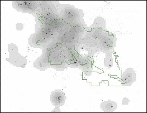
We initially established a change threshold of ±4 SD from the mean using visual inspection and co-spectral plots of the satellite change images with their corresponding PDEQ dust inspection points and kernel density plots. Figure 5 displays the 2005–2004 change image presented as a binary image using the ±4 SD criterion. Pixels meeting the change threshold criterion are assigned black, and the corresponding PDEQ inspection kernel density plot overlain in grayscale.

Figure 5. The remote-sensing-derived change layer is converted to a binary image, with pixels exhibiting change values beyond ±4 SD displayed in black, and all other pixels displayed in white. The black pixels show greatest change signal between the two dates. The PDEQ dust inspection kernel density layer is shown in shades from white to dark gray with increasing density. Both data sets cover the period between June 2004 and May 2005.

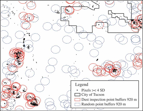
To fine-tune selection of the band difference change threshold and to quantitatively assess model performance, we compared capture rates of thresholded change pixels by sets of buffers around the PDEQ dust inspection points to those of buffers around a set of equal number of random points. We used a 920-m radius buffer size for all sets, which was derived from the average disturbance area reported in the PDEQ dust inspection data set (460 m) with a factor of two in radius applied to ensure the inclusion of the full possible range of disturbance around any one dust inspection point. Buffer sets were generated for each of the four annual periods with PDEQ data (2002–2006), with an example shown in Figure 6.

Figure 6. Demonstration of the buffer technique to assess model performance using the 2004–2003 data sets. Pixels meeting change criteria are shown as black polygons. 920-m buffers are shown in red (solid) lines around PDEQ dust inspection locations, and in blue (dotted) lines for random points. Capture rates of the change pixels are compared for the two buffer data sets to assess model performance.

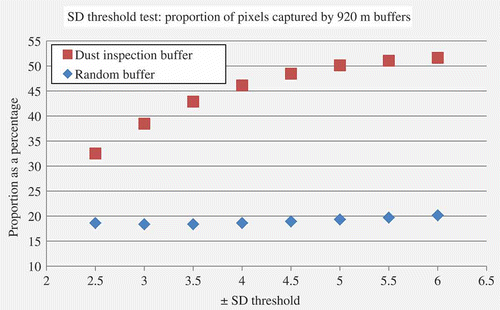
We prepared a set of change images consisting of pixels thresholded from ±2.5 through 6.0 SD from the mean, in increments of 0.5, for the four annual periods with dust inspection data. The capture rates or PDEQ buffers are compared with those of random points in Figure 7, with increasing threshold values.

Figure. 7. Proportion of Landsat TM band 5 image-differenced change pixels captured by buffers (920 m) around county dust inspection points versus the proportion captured by an equal number of buffers around random points, compared at successively increasing standard deviation threshold. Values represent the average of four annual periods from 2003 to 2002 through 2006 to 2005.

3. Results

3.1. Change threshold identification

The capture rate efficiency of thresholded change pixels by the PDEQ dust inspection buffers, compared to random buffers of the same size, increases as the standard deviation threshold increases, until approximately at ±5 SD of the mean, where it plateaus (see Figure 7). We therefore selected ±5 SD of the mean as the optimum threshold.

Using this criterion, we classified the four change images of the annual periods with matching PDEQ data, and the average percentage of change pixels captured by the 920-m PDEQ dust inspection buffers was 50.13%, compared to 19.33% captured by the same number of random point buffers. Compared to random point buffers at the same size, each PDEQ dust inspection buffer captured statistically significantly more change pixels (p < 0.0001, Mann–Whitney rank sum U-test, difference in medians) for each of the comparisons. A summary of statistical comparisons is provided in Tables 2 and 3.

Table 2. Proportional comparison.

Year	Total DEQ or random points	Total change pixels	Pixels inside 920 m buffers DEQ points	Pixels inside 920 m buffers random points
2003–2002	273^a	14,449	5148/14,449 35.63%	1387/14,449 9.60%
2004–2003	1043	19,104	12,945/19,104 67.76%	5469/19,104 28.63%
2005–2004	1013	31,434	16,504/31,434 52.50%	9018/31,434 28.69%
2006–2005	444^a	21,272	9492/21,272 44.62%	2216/21,272 10.42%
Average			50.13% (CV 0.27)	19.33% (CV 0.56)
Notes: Capture rates of satellite change pixels meeting threshold criteria (±5 SD) by 920-m buffers around the Pima County Department of Environmental Quality (PDEQ) permit dust inspection points, as compared to buffers around the same number of random points, for June through May annual periods.
^aPartial year data sets: six months of inspection points only.

Table 3 Difference of means statistical tests.

Mann–Whitney U-test (nonparametric)	Unpaired t-test
p < 0.0001	p < 0.0001 (two-tailed; extremely statistically significant)
U A = 98581.5	Difference of means = 69.10
z = 31.48	95% confidence interval of difference: from 62.99 to 75.22
Mean ranks 1422.7 vs. 604.3	Mean: 79.96 (DEQ buffers) vs. 10.86 (random point buffers)
N 1 = N 2 = 1013	SD: 86.55 vs. 48.19
	SEM: 2.72 vs. 1.51
	N: 1013
Note: Example summary statistics for the 2005–2004 annual period comparing change pixel inclusion rates by PDEQ inspection point buffers (group A) as compared to those of random point buffers (group B).

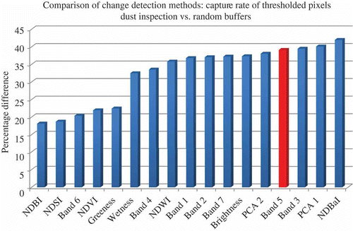
To test our choice of change detection method, we applied the threshold criterion, established for TM band 5 differencing, to products of several other change detection methods, including differencing of other Landsat bands, spectral index differencing and spectral transformation approaches. We subjected each output to the PDEQ and random buffer test. Figure 8 compares TM band 5 differencing with several other change detection methods for one annual period (2004–2003). At least at this criterion TM band 5 differencing in the MIR is among the highest performers, each within a range of 38–42% of superior capture rate efficiency of PDEQ inspection buffers compared to random buffers.

Figure 8. Comparison of change detection techniques. All methods are image differencing of Landsat TM bands or spectral indices, except for the spectral transformation approaches principal component analysis (PCA) and Kauth–Thomas transformation layers. The difference between the percentage of change pixels meeting threshold criteria (±5 SD of the mean) that are captured by 920-m buffers around a set of county dust inspection points to those captured by an equal number of random point buffer are shown. Data were compiled from the 2004–2003 annual change image.

Both qualitative and quantitative accuracy assessments show good cross-correlation between the Landsat TM change detection protocols and PDEQ dust inspection data. This is an important finding: although dust inspection permits go back only a few years, the Landsat TM time series extends back to the mid-1980s. We thus have an excellent historical record of surface disturbance for modeling purposes.

3.2. Change area determination

Change image pixels meeting the criterion of ±5 SD from the change image mean are classified as likely sources of construction-related soil disturbance based on their spatial and statistical association to fugitive dust inspection data. We use the output as a metric to estimate spatial and temporal aspects of the data set.

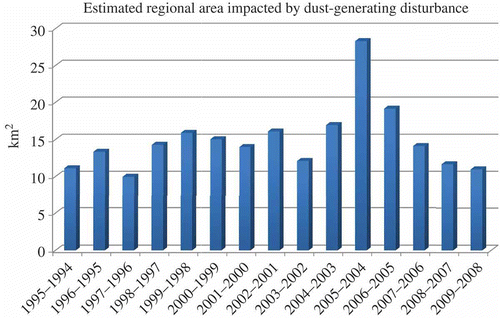
Using the dimensions of the TM band 5 pixel (900 m²), we are able to estimate the surface area impacted by construction-related disturbance in the study area. The values for each annual period during the 15-year span of the study are shown in Figure 9. Estimates ranged from 10.0 (1996–1997) to 28.3 km² (2004–2005), or 0.16–0.44% of the masked study area, respectively. The model estimates that construction-related soil disturbance in eastern Pima County was fairly consistent before 2002, increased successively in the years 2002–2005 to a peak in 2005–2006, and decreased in recent years to pre-peak values.

Figure 9. The aggregated area affected by construction-related soil disturbance likely to generate fugitive dust in the study area for years between 1994 and 2009 is estimated. Disturbance areas are determined by summing pixels meeting threshold criteria: beyond ±5 SD of the mean in the Landsat TM band 5 difference image.

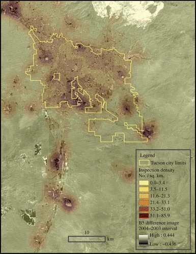
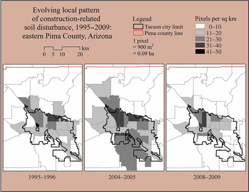
We enumerated the thresholded change pixels to zip code spatial units with areal normalization for each annual period to assess subregional characteristics of the data set. Regional maps of three annual periods covering the span to the study period, with zip code areas experiencing increasing soil disturbance shown in increasing gray scale, are shown in Figure 10. We estimate locally high intensity of construction-related soil disturbance in the urban growth boundary zone of the peripheral north and northwest side of Tucson over the period of study, and increased local disturbance on the south side in the middle of the current decade.

Figure 10. Remote-sensing pixels meeting change criteria likely to indicate fugitive dust sources are aggregated to zip code areal units and normalized by area for three representative annual periods over the span of the study. Aggregation to smaller areal units enables locating hot spots of intense construction-related soil disturbance, and to monitor local trends in the region as a whole.

4. Discussion

4.1. Interfering activities

Surface changes generated from agriculture and mining activities such as crop rotation, field fallowing, mining pond flooding, and range and forest fires were outside the scope of the study. These activities generated significant change signals in some portions of the study area. Our approach was to mask out these areas; they affected only a small portion of study area and were easily isolated using ancillary land-cover maps. Accurate ground-truth data, ancillary data, and additional data processing time and effort may be necessary to perform masking.

4.2. Comparisons to other work

We factor out seasonality using annual-date images, and we are thus provided with a yearly snapshot to capture the activity of a typical residential or commercial construction project cycle (6 months for one single family home or 11 months for a commercial site, EPA 1999). At this resolution, we are likely capturing the construction cycle and its dust-generating propensity as a whole, as opposed to characterizing individual stages. The 16-day repeat cycle for Landsat TM images provides numerous opportunities for scene selection.

Our use of image differencing to detect land-cover change at the urban growth boundary is consistent with previous literature (Fung 1990; Ridd and Liu 1998; Royal 1980; Toll, Royal, and Davis 1980). We report superior results using MIR differencing; many of the early studies emphasized use of the red spectral region. In our case, the pre-change land cover of the Sonoran Desert is anticipated to have a much stronger soil component than that of the other studies (i.e., grassland in Denver, CO, or agriculture fields in Ontario, Canada, and Salt Lake City, UT). We suggest that MIR is equally suited to detect the transformation of a pixel consisting of a significant soil component during disturbance, rearrangement, and subsequent construction.

An additional benefit of the MIR spectral region over visible spectral regions is its known resistance to the affects of atmospheric scattering. The COST model atmospheric adjustments we determined for the MIR images were consistently near zero; our results show that in the case of Landsat TM band 5, minimal preprocessing is necessary. Image differencing of a single spectral band requires minimal preprocessing compared to differencing of spectral indices and other spectral transformations such as principal component analysis.

We arrived at a rigorous image differencing change threshold (5 SD); previous work (Fung 1990; Ridd and Liu 1998; Quarmby and Cushnie 1989) arrived at less stringent thresholds (0.7–1.2 SD). We optimized our output to identify likely source areas of soil disturbance and fugitive dust generation; we can hypothesize that a more stringent criterion is needed to threshold change from a highly soil-dominated pixel characteristic of the Sonoran Desert to another form of soil (i.e., disturbed), than change from predominately agriculture or rangeland land cover. GIS-based modeling methods that test continuous thresholds and use genetic algorithm approaches to optimize moving threshold windows are explored in recent literature to automate and improve binary change detection performance (Im et al. 2008; Im, Rhee, and Jensen 2009; Im, Lu, and Jensen 2011).

4.3. Assessment of accuracy

Our use of PDEQ fugitive dust inspection data with GIS techniques to guide development of the remote-sensing method relies on its accuracy. This appears to be a good choice, but assumptions are made. Foremost is that the inspections point to the occurrence and location of dust-generating activities. This is a straightforward assumption. In addition, we assume that the relationship between department inspections and dust-generating activity is quantifiable. Dust inspections by PDEQ are quantifiable, as supported by discussions with PDEQ staff, in terms of repeat coverage based on duration and scope of the project at any particular site. Finally, we assume that the fugitive dust inspection program assesses all significant soil disturbance sources that generate dust. In this case, remote-sensing methods may serve a role in assessing and validating administrative programs and policy.

Implicit in our method is that every pixel meeting threshold criteria equates to dust-generating activity. We validate our approach using comparisons of the capture rates by buffers around known dust sources to those around random points. Based on our capture rates, we can say we are at least 50% accurate. In one sense, the model will likely overestimate the amount of area affected by soil disturbance, as not all change meeting criteria is due to construction, and not all construction phases are inherently dust-generating. The model may also underestimate this parameter, as change signals occurring on a surface area less than two times the pixel size of Landsat TM (30 m) may not identified. Considering these limitations, the model may be best suited to compare relative change occurring year-to-year.

4.4. Potential applications of the output

Recent changes in policy and technology, including open access to the Landsat imagery archive, web browser tools and software that enable interactive viewing of change imagery, and tools that perform auto-thresholding for change detection, have brought remote-sensing change detection functionality to a broad range of users (Exelis 2012; Green 2011; Warner, Almutairi, and Lee 2009). Binary change images can provide information which is useful for planning and management purposes, especially when quick overview products are needed as preliminary output (Im, Lu, and Jensen 2011). The 30-m emission source metric reported here is in raster format, and it is easily converted to grid or GIS-based output at various scales and denominational units.

This output enables the assessment of the contribution of construction-related activities to total fugitive dust emissions, and it is a potential substitute or validation data for emission inventory data (EPA 2012b, 2012d). The characterization of the spatial density of emissions sources and their respective contributions (via emission factors) to fugitive dust provide a means for independent assessment of the efficiency of fugitive dust controls, abatement strategies and regulations. Similarly, we suggest that the output may also be useful for substitution and validation of methods employing source apportionment of PM monitoring network data. We, in addition, plan to use the output to characterize source areas of Coccidioides spp. spore propagation.

5. Conclusion

We employed remote sensing and GIS techniques to characterize construction-related soil disturbance likely to generate fugitive dust for an arid region of the United States. Image differencing of the Landsat TM band 5 (MIR), with a change threshold of ±5 SD of the mean, suitably estimates the location and area affected by construction-related soil disturbance in southern Arizona. We validated our method by comparison of capture rates of change pixels by buffers around known dust sources to those of an equal number of random points (50.13% vs. 19.33%, respectively, statistically significant difference). We estimate annual area affected by construction-related change, with values ranging from 10.0 (1996–1997) to 28.3 km² (2004–2005), or 0.16–0.44% of the masked study area, respectively. We aggregate this metric to zip code areas and identify regional hot spots and regional trends of the 15-year study period.

The remote-sensing approach described here is simple, requires minimal image preprocessing and processing, and makes use of readily accessible, free data. It locates areas of intense dust-generating activity for monitoring and mitigating fugitive dust. The spatially explicit output may serve as input or validation of models predicting the construction-related fugitive dust contribution to ambient air pollution, to perform atmospheric dispersion modeling, and to predict the dissemination of soil-borne pathogens such as the Coccidioides fungus.

Acknowledgments

Components of this research were funded with a grant from the Science to Achieve Results (STAR) program of the U.S. Environmental Protection Agency (#R8327540). Special thanks are extended to the Pima County Department of Environmental Quality for assistance with their dust inspection database and data collection methodology, and to the Arizona Regional Image Archive (ARIA) for assistance with COST image preprocessing protocol. Additional appreciation is extended to Dr. Daoqin Tong of the School of Geography and Development at the University of Arizona for assistance with statistical methods.

References

- AIA. 2007. “Tucson/Pima County, Arizona: One Million Reasons to Plan for Sustainable Growth.” Southern Arizona Chapter of the American Institute of Architects. http://www.aia.org/aiaucmp/groups/aia/documents/pdf/aias078092.pdf (http://www.aia.org/aiaucmp/groups/aia/documents/pdf/aias078092.pdf) (Accessed: 17 June 2013 ).
- Census, 2012. “State & County QuickFacts, Pima County, Arizona.” U.S. Census Bureau. http://quickfacts.census.gov/qfd/states/04/04019.html (http://quickfacts.census.gov/qfd/states/04/04019.html)
- Chander , G. , Markham , B. L. and Helder , D. L. 2009 . Summary of Current Radiometric Calibration Coefficients for Landsat MSS, TM, ETM+, and EO-1 ALI Sensors . Remote Sensing of Environment , 113 : 893 – 903 .
- Chavez , P. S. Jr. 1996 . Image-Based Atmospheric Corrections – Revisited and Improved . Photogrammetric Engineering & Remote Sensing , 62 ( 9 ) : 1025 – 1036 .
- Chen , W. , Liu , L. , Zhang , C. , Wang , J. , Wang , J. and Pan , Y. 2004 . Monitoring the Seasonal Bare Soil Areas in Beijing Using Multi-Temporal TM Images . Proceedings of 2004 IEEE International Geoscience and Remote Sensing Symposium , 5 : 3379 – 3382 .
- Chow , J. C. , Watson , J. G. , Ashbaugh , L. L. and Magliano , K. L. 2003 . Similarities and Differences in PM10 Chemical Source Profiles for Geologic Dust from the San Joaquin Valley, California . Atmospheric Environment , 37 ( 9–10 ) : 1317 – 1340 .
- Coppin , P. , Jonckheere , I. , Nackaerts , K. , Muys , B. and Lambin , E. 2004 . Digital Change Detection Methods in Ecosystem Monitoring: A Review . International Journal of Remote Sensing , 25 ( 9 ) : 1565 – 1596 .
- Elconin , A. F. , Egeberg , R. O. and Egeberg , M. C. 1964 . Significance of Soil Salinity on the Ecology of Coccidioides Immitis . Journal of Bacteriology , 87 ( 3 ) : 500 – 503 .
- Emmons , C. W. 1942 . Coccidioidomycosis . Mycologia , 34 ( 4 ) : 452 – 463 .
- EPA. 1995. “Introduction to Fugitive Dust Sources.” Chap. 13.2 in AP-42, Compilation of Air Pollutant Emission Factors. Washington, DC: U.S. Environmental Protection Agency. http://www.epa.gov/ttn/chief/ap42/index.html#toc (http://www.epa.gov/ttn/chief/ap42/index.html#toc)
- 1999 . “Estimating Particulate Emissions from Construction Operations, Final Report ” . In Prepared for the Emission Factor and Inventory Group, Office of Air Quality Planning and Standards by the Midwest Research Institute, Kansas City, MO, EPA contract no. 68-D7-0068. , Research Triangle Park , NC : U.S. EPA .
- EPA. 2003. “Particle Pollution and Your Health.” Office of Air and Radiation, U.S. Environmental Protection Agency, EPA-452/F-03-001. http://www.epa.gov/pm/pdfs/pm-color.pdf (http://www.epa.gov/pm/pdfs/pm-color.pdf) (Accessed: 17 June 2013 ).
- EPA. 2012a. “FIP Rule Definitions.” U.S. Environmental Protection Agency, Pacific Southwest, Region 9. http://www.epa.gov/region9/air/phoenixpm/define.html (http://www.epa.gov/region9/air/phoenixpm/define.html) (Accessed: 17 June 2013 ).
- EPA. 2012b. “The National Emissions Inventory: 2008 National Emissions Inventory Data.” U.S. Environmental Protection Agency, Technology Transfer Network, Clearinghouse for Inventories & Emission Factors. http://www.epa.gov/ttn/chief/net/2008inventory.html (http://www.epa.gov/ttn/chief/net/2008inventory.html) (Accessed: 17 June 2013 ).
- EPA. 2012c. “The Green Book Nonattainment Areas for Criteria Pollutants.” U.S. Environmental Protection Agency. http://www.epa.gov/airquality/greenbook/ (http://www.epa.gov/airquality/greenbook/) (Accessed: 17 June 2013 ).
- EPA. 2012d. “NEI Browser: County Emissions.” U.S. Environmental Protection Agency, National Emissions Inventory, NEI Browser. http://www.epa.gov/ttn/chief/eiinformation.html (http://www.epa.gov/ttn/chief/eiinformation.html) (Accessed: 17 June 2013 ).
- Exelis ENVI EX Image Differencing . 2012 . ENVI EX Tutorial: Image Difference Change Detection, 9. , Boulder , CO : Exelis Visual Information Solutions .
- Field , J. P. , Belnap , J. , Breshears , D. D. , Neff , J. C. , Okin , G. S. , Whicker , J. J. , Painter , T. H. , Ravi , S. , Reheis , M. C. and Reynolds , R. L. 2010 . The Ecology of Dust . Frontiers in Ecology and the Environment , 8 ( 8 ) : 423 – 430 .
- Fung , T. 1990 . An Assessment of TM Imagery for Land-Cover Change Detection . IEEE Transactions on Geoscience and Remote Sensing , 28 ( 4 ) : 681 – 684 .
- Galgiani , J. N. 1999 . Coccidioidomycosis: A Regional Disease of National Importance . Annals of Internal Medicine , 130 ( 4 ) : 293 – 300 .
- Gao , B. 1996 . NDWI – A Normalized Difference Water Index for Remote Sensing of Vegetation Liquid Water from Space . Remote Sensing of Environment , 58 ( 3 ) : 257 – 266 .
- Green , K. 2011 . Change Matters . Photogrammetric Engineering & Remote Sensing , 77 ( 4 ) : 305 – 309 .
- Hardisky , M. A. , Smart , R. M. and Klemas , V. 1983 . Seasonal Spectral Characteristics and Aboveground Biomass of the Tidal Marsh Plant, Spartina alterniflora . Photogrammetric Engineering and Remote Sensing , 49 ( 1 ) : 85 – 92 .
- He , C. , Shi , P. , Xie , D. and Zhao , Y. 2010 . Improving the Normalized Difference Built-Up Index to Map Urban Built-Up Areas Using a Semiautomatic Segmentation Approach . Remote Sensing Letters , 1 ( 4 ) : 213 – 221 .
- Ho , K. F. , Lee , S. C. , Chow , J. C. and Watson , J. G. 2003 . Characterization of PM10 and PM2.5 Source Profiles for Fugitive Dust in Hong Kong . Atmospheric Environment , 37 ( 8 ) : 1023 – 1032 .
- Howarth , P. J. and Wickware , G. M. 1981 . Procedures for Change Detection Using Landsat Digital Data . International Journal of Remotes Sensing , 2 ( 3 ) : 277 – 291 .
- Im , J. , Lu , Z. and Jensen , J. R. 2011 . A Genetic Algorithm Approach to Moving Threshold Optimization for Binary Change Detection . Photogrammetric Engineering & Remote Sensing , 77 ( 2 ) : 167 – 180 .
- Im , J. , Rhee , J. and Jensen , J. R. 2009 . Enhancing Binary Change Detection Performance Using a Moving Threshold Window (MTW) Approach . Photogrammetric Engineering & Remote Sensing , 75 ( 8 ) : 951 – 962 .
- Im , J. , Rhee , J. , Jensen , J. R. and Hodgson , M. E. 2008 . Optimizing the Binary Discriminant Function in Change Detection Applications . Remote Sensing of Environment , 112 : 2761 – 2776 . 2008
- Ingram , K. , Knapp , E. and Robinson , J. W. 1981 . Change Detection Technique Development for Improved Urbanized Area Delineation, 75. Technical Memorandum, CSC/TM-81/6087. , Silver Spring , MD : Computer Sciences Corporation .
- ISO . 1994 . “ Air Quality – General Aspects, Vocabulary ” . In In ISO Standard 4225, International Organization for Standardization (ISO), ISO TC 146/SC 4. , Geneva : International Organization for Standardization .
- Jackson , T. J. , Chen , D. , Cosh , M. , Fuqin , L. , Anderson , M. , Walthall , C. , Doriaswamy , P. and Hunt , E. R. 2004 . Vegetation Water Content Mapping Using Landsat Data Derived Normalized Difference Water Index for Corn and Soybeans . Remote Sensing of Environment , 92 ( 4 ) : 475 – 482 .
- Jensen , J. R. 2005 . Introductory Digital Image Processing: A Remote Sensing Perspective, 526. , 3rd ed. , Upper Saddle River : NJ: Prentice-Hall .
- Jensen , J. R. , Cowen , D. , Althausen , J. , Narumalani , S. and Weatherbee , O. 1993 . An Evaluation of Coast Watch Change Detection Protocols in South Carolina . Photogrammetric Engineering & Remote Sensing , 59 ( 6 ) : 1039 – 1046 .
- Jensen , J. R. and Im , J. 2007 . “ Remote Sensing Change Detection in Urban Environments ” . In Geo-Spatial Technologies in Urban Environments Policy, Practice, and Pixels , 2nd ed. , Edited by: Jensen , R. R. , Gatrell , J. D. and McLean , D. D. 7 – 32 . Berlin : Springer-Verlag .
- Jensen , J. R. and Toll , D. L. 1982 . Detecting Residential Land-Use Development at the Urban Fringe . Photogrammetric Engineering and Remote Sensing , 48 ( 4 ) : 629 – 643 .
- Kirkland , T. N. and Fierer , J. 1996 . Coccidioidomycosis: A Reemerging Infectious Disease . Emerging Infectious Diseases , 3 ( 2 ) : 192 – 199 .
- Kolivras , K. N. , Johnson , P. S. , Comrie , A. C. and Yool , S. R. 2001 . Environmental Variability and Coccidioidomycosis (Valley Fever) . Aerobiologia , 17 : 31 – 42 .
- Kong , S. , Ji , Y. , Lu , B. , Chen , L. , Han , B. , Li , Z. and Bai , Z. 2011 . Characterization of PM10 Source Profiles for Fugitive Dust in Fushun-A City Famous for Coal . Atmospheric Environment , 45 : 5351 – 5365 .
- Maddy , K. 1957 . Ecological Factors of the Geographic Distribution of Coccidioides Immitis . Journal of the American Veterinary Medical Association , 130 : 475 – 476 .
- Maki , M. , Ishiahra , M. and Tamura , M. 2004 . Estimation of Leaf Water Status to Monitor the Risk of Forest Fires by Using Remotely Sensed Data . Remote Sensing of Environment , 90 : 441 – 450 .
- McFeeters , S. K. 1996 . The Use of the Normalized Difference Water Index (NDWI) in the Delineation of Open Water Features . International Journal of Remote Sensing , 17 ( 7 ) : 1425 – 1432 .
- NASA. 2012a. “Remote Sensing Overview Presentation.” U.S. Geological Service. Washington, DC: U.S. Department of the Interior. http://l7downloads.gsfc.nasa.gov/assets/other/RSI_notes.pdf (http://l7downloads.gsfc.nasa.gov/assets/other/RSI_notes.pdf)
- NASA. 2012b. “The Thematic Mapper, National Aeronautics and Space Administration.” Washington, DC: NASA. http://landsat.gsfc.nasa.gov/about/tm.html (http://landsat.gsfc.nasa.gov/about/tm.html)
- Pappagianis , D. and Einstein , H. 1978 . Tempest from Tehachapi Takes Toll or Coccidioides Conveyed Aloft and Afar . Western Journal of Medicine , 127 : 527 – 530 .
- Park , J. B. , Siegel , K. , Vaz , V. , Komatsu , K. , McRill , C. , Phelan , M. and Colman , T. 2005 . An Epidemic of Coccidioidomycosis in Arizona Associated with Climatic Changes, 1998–2001 . The Journal of Infectious Diseases , 191 : 1981 – 1987 .
- Pima. 2012. “Fugitive Dust FAQs,” Pima County, Arizona. http://www.deq.pima.gov/air/FugitiveDustFAQs.htm (http://www.deq.pima.gov/air/FugitiveDustFAQs.htm) (Accessed: 17 June 2013 ).
- Quarmby , N. A. and Cushnie , J. L. 1989 . Monitoring Urban Land Cover Changes at the Urban Fringe from SPOT HRV Imagery in South-East England . International Journal of Remote Sensing , 10 ( 6 ) : 953 – 963 .
- Ridd , M. K. and Liu , J. 1998 . A Comparison of Four Algorithms for Change Detection in an Urban Environment . Remote Sensing of Environment , 63 : 95 – 100 .
- Rogers , A. S. and Kearney , M. S. 2004 . Reducing Signature Variability in Unmixing Coastal Marsh Thematic Mapper Scenes Using Spectral Indices . International Journal of Remote Sensing , 25 ( 12 ) : 2317 – 2335 .
- Roy , P. S. , Miyatake , S. and Rikimaru , A. October 1997 . “ Biophysical Spectral Response Modeling Approach for Forest Density Stratification ” . In ACRS1997 Proceedings, Asian Conference on Remote Sensing of the Environment , October , 20 – 25 . FR97-7, Kuala Lumpur .
- Royal , J. A. 1980 . Change Detection Method Development Census Urban Area Application Pilot Test , 74 p Beltsville , MD : Final Report, Contract NAS5-25707, General Electric Company .
- Samara , C. 2005 . Chemical Mass Balance Source Apportionment of TSP in a Lignite-Burning Area of Western Macedonia, Greece . Atmospheric Environment , 39 ( 34 ) : 6430 – 6443 .
- Schneider , E. , Hajjeh , R. A. , Spiegel , R. A. , Jibson , R. W. , Harp , E. L. , Marshall , G. A. and Gunn , R. A. 1997 . A Coccidioidomycosis Outbreak Following the Northridge, Calif, Earthquake . The Journal of the American Medical Association , 277 ( 11 ) : 904 – 908 .
- Silverman , B. W. 1986 . Density Estimation for Statistics and Data Analysis , 176 p New York : Chapman and Hall .
- Stefanov , W. L. , Ramsey , M. S. and Christensen , P. R. 2003 . Identification of Fugitive Dust Generation, Transport, and Deposition Areas Using Remote Sensing . Environmental & Engineering Geoscience , IX ( 2 ) : 151 – 165 .
- Swatek , F. E. 1970 . Ecology of Coccidioides Immitis . Mycopathologia et Mycologia Applicata , 40 : 3 – 12 .
- SWReGAP. 2004. “Provisional Digital Land Cover Map for the Southwestern United States,” Version 1.0, USGS National Gap Analysis Program, RS/GIS Laboratory, College of Natural Resources, Utah State University. http://earth.gis.usu.edu/swgap/landcover.html (http://earth.gis.usu.edu/swgap/landcover.html)
- Toll , D. L. , Royal , J. A. and Davis , J. B. 1980 . “ Urban Area Update Procedures Using Landsat Data ” . In Proceedings of the American Society of Photogrammetry, ASP Fall Technical Meeting Bethesda , MD RS-E-1-17, 12.
- USGS. 2010. “Frequently Asked Questions about the Landsat Missions.” U.S. Geological Service, U.S. Department of the Interior. http://landsat.usgs.gov/best_spectral_bands_to_use.php (http://landsat.usgs.gov/best_spectral_bands_to_use.php) (Accessed: 17 June 2013 ).
- USGS. 2011. “Opening the Landsat Archive/Product Specifications.” U.S. Geological Service, U.S. Department of the Interior. http://landsat.usgs.gov/products_data_at_no_charge.php (http://landsat.usgs.gov/products_data_at_no_charge.php) (Accessed: 17 June 2013 ).
- Warner , T. A. , Almutairi , A. and Lee , J. Y. 2009 . “ Remote Sensing of Land Cover Change ” . In The Sage Handbook of Remote Sensing , Edited by: Warner , T. A. , Nelllis , M. D. and Foody , G. M. 459 – 472 . Los Angeles , CA : Sage .
- Watson , J. G. , Zhu , T. , Chow , J. C. , Engelbrecht , J. , Fujita , E. M. and Wilson , W. E. 2002 . Receptor Modeling Application Framework for Particle Source Apportionment . Chemosphere , 49 ( 9 ) : 1093 – 1136 .
- Werner , S. B. 1974 . Coccidioidomycosis Among Archeology Students: Recommendations for Prevention . American Antiquity , 39 ( 2 ) : 367 – 370 .
- Wilson , E. H. and Sader , S. A. 2002 . Detection of Forest Harvest Type Using Multiple Dates of Landsat TM Imagery . Remote Sensing of Environment , 80 ( 3 ) : 385 – 396 .
- Zha , Y. , Ga , J. and Ni , S. 2003 . Use of Normalized Difference Built-Up Index in Automatically Mapping Urban Areas from TM Imagery . International Journal of Remote Sensing , 24 ( 3 ) : 583 – 594 .
- Zhao , H. and Chen , X. July 2005 . “ Use of Normalized Difference Bareness Index in Quickly Mapping Bare Areas from TM/ETM+ ” . In Proceedings of IEEE International Geoscience and Remote Sensing Symposium (IGARSS '05) Vol. 3 , July , 25 – 29 . Seoul , Korea