
Abstract
Satellite remote sensing is an essential tool for crop monitoring over large areas. One of the most practical issues is defining the appropriate spatial resolution level in terms of technical aspects such as orbit path, swath width, or revisit rate, particularly in South Korea where the major agricultural activity of rice cultivation is conducted mostly by private farmers on small parcels of land. This study is an experimental approach to examine the sensitivity of vegetation indices of three paddy rice crops at various spatial resolutions during two seasons (July, September) using RapidEye multi-spectral image data. The results showed that lower spatial resolutions (beyond 26 m) had higher uncertainty for reflecting homogeneous field conditions and differentiating crop species. We stress, however, that the appropriate resolution might be dependent on the actual paddy size in the fields. Regarding the phenology of rice plants, the spectral difference of vegetation indices was more dependent on the same spatial resolution in July than in September. In addition, the July imagery, in which the vegetative and reproductive growth stages of the various rice cultivars were mixed, was slightly more effective for differentiating paddy rice crop classes. As an additional benefit, provision by RapidEye of red-edge spectral information ensured that a transformed vegetation index that made use of the red-edge band, which was edgNDVI in this study, was more applicable for differentiating three paddy rice crops in homogeneous rice cultivation.
1. Introduction
One of the sectors most vulnerable to global climate change is agriculture. Temperature and precipitation changes have affected crop growth, yields, and the areas suitable for agriculture. Unexpected, extreme droughts and floods often cause crop damage on vast scales, resulting in crop-price instability, the so-called agflation (Easterling et al. Citation2000; Park and Lee Citation2008; Kang, Khan, and Ma Citation2009; Mestre-Sanchís and Feijóo-Bello Citation2009). National food security, therefore, depends greatly on effective decision-making based on rigorous crop forecasting supported by rapid and accurate information (Wu and Li Citation2012). In addition, increasing environmental and conservation concerns demand better farm management regarding use of fertilizers, herbicides, seed, and fuel. Precision agriculture based on advances in information technology is now increasingly common worldwide (Mondal and Basu Citation2009; Mulla Citation2013).
Despite the advantages of satellite remote sensing in mapping crop areas and large-scale crop condition monitoring (Frohn Citation2005; Xiao et al. Citation2006; Castillejo-González et al. Citation2009; Gumma et al. Citation2011; Chen, Chen, and Son Citation2012; Wu and Li Citation2012; Long et al. Citation2013), the high spectral variability in crop species, growth stages, health conditions, soil, water content, and microclimate hampers the application of remote sensing to agriculture (Peña-Barragán et al. Citation2011). The recent advances in satellite remote sensing technology have opened up new perspectives by offering high spatial and spectral resolution as well as rapid revisit rates (up to daily). In particular, satellite missions, such as RapidEye and WorldView-2, have shown potential for estimating the chlorophyll content for crop monitoring due to their ability to monitor the red-edge spectral band (Filella and Penuelas Citation1994; Eitel et al. Citation2011; Kim and Yeom Citation2014).
In South Korea, agricultural lands are operated mostly by private farmers on small parcel units, which often differ in seeding, crop dusting, and harvesting periods. Crop conditions usually depend on the individual owner’s management skills. This circumstance increases the need for high-resolution data to gather precise, up-to-date information on crop conditions. However, coverage of wide areas is also required for public management planning for disease treatment, production estimation, and compensation measures at the regional or national level. Previous studies also indicated that determining which sensors offer the appropriate spatial, spectral, temporal, and radiometric scales to meet specific mapping needs may not be a simple task as multiple criteria must be considered and evaluated (Phinn Citation1998; Maxwell et al. Citation2014). It is therefore worthwhile to define the optimal spatial resolution at which the spectral characteristics of crop landscapes can be differentiated without complicated data processing, which requires excessive high-spatial-resolution imagery. Cost-effective crop information systems can then be realized with rapid data processing.
As the spatial resolution depends on orbital height, swath width, and the revisit rate of the satellite due to satellite system design (Wertz and Larson Citation1999), high spatial resolution and wide-area coverage with a rapid revisit rate are often conflicting criteria for satellite-remote-sensing-based crop monitoring projects. Generally, earth observation satellites with very high spatial resolutions, such as KOMPSAT-3, GeoEye, and WorldView, are designed to view only relatively narrow swaths, such that data acquisition over a wide area in short periods is difficult. In contrast, satellites such as MODIS that offer daily imagery have the advantage of very fast revisit rates and wide-area coverage, but they are restricted by their low spatial resolution (~250 m or less), such that precise spectral characteristics representing homogeneous crop field conditions cannot be obtained (Ozdogan and Woodcock Citation2006; Karkee et al. Citation2009).
In South Korea, paddy rice cultivation is the main agricultural activity, and the rice cultivars grown in South Korea can be grouped into early maturing, medium-maturing, and medium-late-maturing rice based on heading period or growing days (Park Citation2014). Due to regional climate and geographic conditions, early, medium-, and medium-late-maturing rice cultivars are transplanted at different times, at an interval of ~7–10 days. Therefore, rice cultivars can be roughly differentiated by their transplanting periods, which can be determined by the relative growth differences of rice plants at a particular time point. The rice yield can then be estimated before the harvest, based on the average productivity of each rice cultivar (Hossain et al. Citation2003; Gutierrez, Kim, and Kim Citation2013; NICS Citation2014). However, the ability to detect fine-scale growth differences of rice plants depends mainly on the spatial resolution but also on the spectral resolution.
The vegetation indices are conceived based on the fact that vegetation leaf structures have adapted to perform photosynthesis; hence their interaction with electromagnetic energy has a direct impact on their spectral characteristics. Therefore, vegetation indices are defined as radiometric measures that function as indicators of the relative abundance and activity of green vegetation, percentage of green cover, chlorophyll content, green biomass, and absorbed photosynthetically active radiometer (Running et al. Citation1994; Jensen Citation2000).
In this context, we examined in this study the sensitivity of vegetation indices of three paddy rice cultivars as the spatial resolution degraded gradually. In order to pretend the other influence on the spectral characteristics such as sensor sensitivity or spectral ranges of different satellite systems, we applied one sensor of RapidEye and varied its spatial resolution. We also examined how the phenology of the rice cultivars influences the spectral characteristics at different spatial resolutions by analyzing two season’s RapidEye image data. In addition, regarding the spectral resolution, as RapidEye multispectral satellite sensor offers an additional spectral range of red-edge, we applied different kinds of vegetation indices adopting the red-edge spectral band.
2. Study area, data, and methods
2.1 Description of the study area
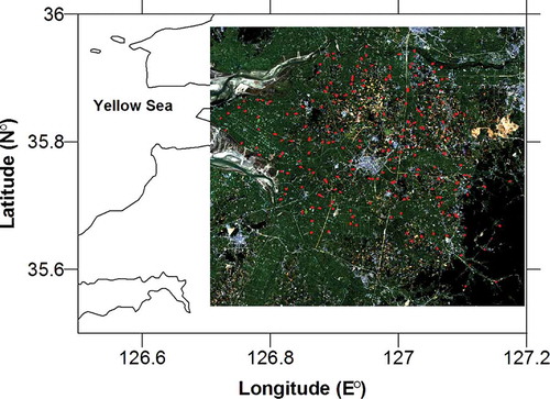
Kimje Province, which is located in southwestern South Korea, is famous for its rice paddy-dominated agriculture. It produces 1/40th of the national rice yield. The study area in this paper covers ~1300 km2 from 35.53ºN, 126.45ºE (upper left) to 35.39ºN, 127.05ºE (lower right), and is characterized by relatively wide plains and a moderate marine climate. As in other typical agricultural regions in South Korea, the partitions of agricultural land mostly correspond to rice paddies divided by narrow paths (~1–2 m wide).
In this region, early maturing rice cultivars (late transplanted) are usually transplanted around 13–16 June, develop ears early in August, and are harvested 40–45 days after earing (ca. 15–20 September). Medium-maturing rice cultivars (conventionally transplanted) are usually transplanted around 3–10 June, develop ears in the middle of August, and are harvested 45–50 days after earing (ca. 30 September to 5 October). Medium-late–maturing rice cultivars (early transplanted) are transplanted around 27 May to 5 June, develop ears at the end of August, and are harvested 50–55 days after earing (ca. 15–20 October) (RDA Citation2011a, RDA Citation2011b).
2.2 RapidEye satellite image data
RapidEye, which was launched in August 2008, is a constellation mission consisting of five identical small satellites. It provides high-resolution multispectral imagery in five optical bands corresponding to the blue, green, red, red-edge, and near-infrared (NIR) parts of the electromagnetic spectrum (440–850 nm). The satellites are placed in a single sun-synchronous orbit at an altitude of 630 km. At nadir, the revisit period is 5.5 days, and the ground sampling distance is 6.5 m. If gathered off nadir, imagery can be acquired daily for the same site. The total recording capacity of the five satellites reaches up to 4 million km2 per day, with a swath width of 77 km ().
Table 1. Specifications of RapidEye mission (BlackBridge Citation2013).
Despite an intensive RapidEye satellite image campaign during the entire 2011 growing season, few applicable data were available because of unusually long rainy days and cloudy weather conditions in this summer. However, two satellite images representing different phases of rice plants were obtained. The image gathered in July (19 July 2011) reflects differences in vegetative growth among three rice cultivars, whereas the image in September (22 September 2011) reflects the ripening stage.
2.3 Atmospheric and geometric correction
Two RapidEye images in product type 1 B acquired on 19 July and 22 September 2011 were used for the analysis. The July satellite scene for the study area included some clouds and their shadows, but was haze free. The image for September was recorded under clear weather conditions, without any clouds. For calculation of the surface reflectance, the top of atmosphere (TOA) reflectance was computed by converting digital numbers (DNs) to radiometric values with the presented scale and offset value from RapidEye Meta files. The estimated TOA reflectance was then corrected using a Second Simulation of a Satellite Signal in the Solar Spectrum Vector (6S) atmospheric correction model by inputting the spectral response functions (SRF) of RapidEye multispectral channels, geometric condition, and atmospheric conditions for surface reflectance (Vermote et al. Citation1997). The 1-nm SRF resolution of RapidEye is resampled to a step of 2.5 nm to input into the 6S simulation model. For geometric condition, solar zenith angle, solar azimuth angle, satellite zenith angle, satellite azimuth angle, and date are used for relative sensor–target–sun geometry. In this study, the bidirectional reflectance distribution function (BRDF) model was not considered due to its high spatial resolution. Regarding atmospheric conditions, we utilize the 6S default values to retrieve the surface reflectance considering a standard atmosphere. The mid-latitude summer condition with the maritime aerosol model was selected to reflect the study area environment, which had a moderate marine climate.
After atmospheric correction, a geometric correction was applied using a value-added processing system (VAPS) developed by the Korea Aerospace Research Institute (KARI) with an automatic image-to-image registration method. VAPS is an automatic post-processing system for Ortho, Pan-Sharpening, and Mosaic. The national database of orthorectified KOrea MultiPurpose SATellite (KOMPSAT)-2 images was used as reference data. The relative root-mean-square error (RMSE) between two RapidEye images was less than 1 pixel.
2.4 Sample data collection
For analysis of the changing spectral characteristics, we selected three paddy rice cultivars: early transplanted (medium-late-maturing) rice, conventionally transplanted (medium-maturing) rice, and late-transplanted (early maturing) rice. We randomly selected 180 paddy parcels on the digital land cadaster map at 1:1000 scale and excluded paddy parcels located under or near clouds or their shadow in both RapidEye images (). The exact assignment of these sample paddies for these rice sorts was accomplished by field survey in the first week of August 2011.
Figure 1. Study area: Kimje/Cheonbuk (RapidEye true color composition, acquired on 22 September 2011). Red polygons indicate the sample paddies for analysis (119 paddies).
2.5 Image resolution degradation and calculation of vegetation indices
The atmospherically and geometrically corrected RapidEye satellite images with 6.5-m resolution were degraded successively in 2 × 2 steps, creating new imagery with 13-, 26-, 52-, 104-, and 208-m spatial resolutions. To reduce the spatial resolution of RapidEye, we used the image degradation tool in ERDAS IMAGINE (version 10). This process reduces the resolution of an image by an integer factor in the X and Y direction and averages all of the original ‘small’ pixels that comprise the new ‘big’ pixels using the Image Degradation tool in ERDAS IMAGE 10.0. Vegetation indices were then calculated at each spatial resolution. Besides the widely used normalized difference vegetation index (NDVI), transformed vegetation indices including gNDVI (Green NDVI), NDVIre, and edgNDVI were calculated ().
Table 2. Vegetation indices used in this study.
Vegetation indices are defined as dimensionless, radiometric measures that function as indicators of the relative abundance and activity of green vegetation. More than 20 vegetation indices are in use. Many are functionally equivalent in information content, whereas some provide unique biophysical information (Jensen Citation2000). NDVI is the most widely applied vegetation index calculated by plant ‘greenness’, which can be calculated by considering difference in photosynthetically absorbed radiation between red and NIR (Rouse Citation1974). The other vegetation indices tested in this study are transformed variants of NDVI to examine the benefits of red-edge and green spectral information in detail.
2.6 Segmentation and spectral analysis
To extract paddy units on the RapidEye satellite image at each resolution, we carried out image segmentation using the eCognition Developer software (version 8.64). A segment layer was created that exactly reflected the vector geometry of the paddy parcel extracted from the digital land cadaster map. As the digital cadaster map used in this study was established at the large scale of 1:1000, even very small paddy units were created as image objects. Then, in case that the same rice cultivars were planted in the neighborhoods, these paddies were fused as one paddy unit. After that, the image segments smaller than 100 original pixels (ca. 4200 m2) were eliminated to ensure a reasonable paddy size. In this way, we aimed to obtain sufficient homogeneous pixels in a paddy unit and to make the paddy segment recognizable as spatial resolution degraded to 208 m. We also excluded paddies located under and near clouds or shadows on both images. As a result, 119 objects remained; these served as sample paddies.
The mean values of the four vegetation indices for each paddy segment at each resolution level were calculated. The spectral differences among three paddy rice cultivars representing different growth stages were analyzed using SPSS Statistics (version 17). We conducted a one-way analysis of variance (ANOVA) to compare the mean differences among the three paddy rice groups. For cases of unequal variation, tests of equality of means using the Brown–Forsythe and Welch methods were performed. Then, a post hoc multiple comparison with Duncan’s test (equal variation) and Dunnett’s T3 test (unequal variation) was used to determine whether all three paddy rice classes were independent groups, and, if not, which paddy classes could be grouped in homogeneous subsets.
3. Results
3.1 NDVI analysis
According to the ANOVA, there was significant variation in NDVI at the p < 0.5 level for the three paddy rice classes in both July and September at all resolution levels (). Post hoc comparisons using the Duncan’s test (α 0.05) indicated significant differences in mean values among the three paddy rice classes.
Table 3. Statistics with NDVI by spatial resolution.
In July, the early transplanted rice had the highest NDVI values, followed by the conventionally transplanted and late-transplanted rice, at all resolution levels. In September, the order was reversed. This phenomenon is caused by the phenological growth condition. The paddy rice plants can be differentiated in July by length and density, for example, late-transplanted rice paddies are covered by young rice plants and some parts of the soil as well as irrigation water, whereas early transplanted rice paddies are covered by relatively dense rice plants in the vegetative growth stage after tillering. These characteristics were reflected in the marked differences in the NDVI and other vegetation indices among paddy rice classes in July (). In contrast, the paddy rice plants enter the grain-filling period in September. With the exception of those already harvested, most paddies remained greenish, so that the vegetation indices in September showed minimal differences among paddy rice classes.
Figure 2. Mean comparison of vegetation indices at different spatial resolutions.
As the spatial resolution was reduced, the NDVI of early and conventionally transplanted rice decreased gradually, whereas the NDVI of the late-transplanted rice increased in July. In September, the change in the NDVI, depending on the spatial resolution, was less than that in July, except in the case of the early transplanted rice. Because the early transplanted rice had been harvested by this time and remained as paddy soil, its NDVI values were low at high resolution but increased as the spatial resolution decreased. It is clear that the low values at high spatial resolution reflect not the rice plant but the rice stubble partially covered with paddy soil. But it showed the mixed pixel effect clearly as the spatial resolution degrades. Because the early transplanted rice was planted in small units scattered across the entire paddy landscape, the corresponding pixels of early transplanted paddies were mixed with the neighborhood pixels of still-growing rice plants in the lower resolutions. This explains the rapid increase in the NDVI in early transplanted rice paddies. A particularly rapid increase was observed at resolutions lower than 26 m.
In summary, the NDVI could differentiate the three paddy rice crop classes in both July and September. The spectral difference was distinct at higher spatial resolutions but started to blur at resolutions lower than 52 m ().
3.2 NDVIre analysis
The differences in NDVIre among three paddy rice classes were statistically significant at the 95% level. At spatial resolutions of 104 and 208 m in July, the conventionally and late transplanted rice crops were not differentiated as separate classes (). Otherwise, the general characteristics of the NDVIre would have been similar to those of the NDVI in July and September. Because the NDVIre used the red-edge band instead of the NIR for the calculation, the values were slightly lower than those for the NDVI in general.
Table 4. Statistics with NDVIre by spatial resolution.
3.3 edgNDVI analysis
Results of the one-way ANOVA showed that the three paddy rice crops could be differentiated statistically at the p < 0.5 level of significance using the NDVIre in both July and September at all resolution levels (). In July, the spectral difference gaps among paddy rice classes were gradually decreased markedly at resolutions lower than 26 m, whereas the edgNDVI remained relatively stable despite the changes in spatial resolution in September ().
Table 5. Statistics with edgNDVI by spatial resolution.
3.4 Green NDVI (gNDVI) analysis
Statistically significant differences in gNDVI were found among the three paddy rice classes at the p < 0.5 level (). At relatively lower resolution levels in July, spectral characterization of early and conventionally transplanted rice was difficult, whereas the gNDVI did not indicate differences between conventionally and late-transplanted paddy rice crops at relatively higher resolution levels in September. Therefore, the gNDVI was not useful for differentiating the dissimilar rice crops in rice-dominant paddy fields.
Table 6. Statistics with gNDVI by spatial resolution.
3.5 Segmentation change varies with spatial resolution
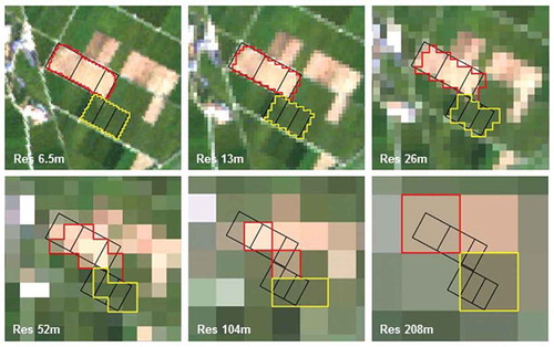
Besides the spectral analysis using vegetation indices, we observed the size and the location of original paddy units in accordance with the degraded spatial resolution. The number of pixels forming a paddy segment with the same cultivar decreased sharply as the spatial resolution degraded (). This implied that very few pixels decide the spectral characteristics at lower spatial resolutions, whereas many pixels can provide a statistical parameterization of the spectral variation at higher resolutions. Hence, at lower resolutions, in cases in which pixels are shifted from the original sample sites, the selected pixels or pixel segments can represent spectral characteristics significantly different from those of the original field. As shows, the segmentation resulted from higher- to lower-resolution shifts at each level, and the traceability of segmentation change decreased markedly from 26- to 52-m resolution and afterwards.
Table 7. Mean number of pixels comprising a paddy segment at each resolution level.
Figure 3. Example of segmentation results as spatial resolution is degraded (red polygon: early transplanted rice, yellow polygon: conventionally transplanted rice, black polygon: paddy units registered in cadaster map).
4. Discussion and conclusion
We examined the sensitivity of vegetation indices verifying paddy rice crops in three rice cultivars corresponding well with the growth stages at two time points (July and September) as the spatial resolution of the satellite images changed. Ozdogan and Woodcock (Citation2006) indicated that insufficient reflection of the agricultural field sizes due to pixel resolution in remotely sensed imagery influences spectral values and hampers the precise classification of cultivated areas. Hence, it is important to determine the optimal spatial resolution for cost-effective crop monitoring. Generally, higher spatial resolution differentiates similar crop species and growth processes better than lower resolution in relatively small, paddy-dominated landscape areas. For most cases in practice, however, high-resolution image data over a wide area of coverage with a short revisit period are not available and require a costly and time-consuming data processing procedure before use. Therefore, for efficient crop monitoring fulfilling the need of private farmers for precise information on their own paddy units, as well as the needs of policy makers for general overview over wide areas, an experimental investigation of the appropriate spatial resolution is warranted. In this study, we suggest three discussion points: (1) what is the appropriate resolution? (2) How does the phenology or crop growth influence the vegetation indices on the same spatial resolution level? (3) What are the advantages of the broad red-edge spectral band for detecting fine differences in similar crop species, as well as condition?
First, regarding the appropriate spatial resolution, this study showed that the difference gap of vegetation indices exhibited the greatest change between 26 and 52 m resolution. Moreover, the shape of segments becomes conspicuously vague going from 26 to 52 m resolution. Therefore, spatial resolutions lower than 26 m fail to reflect homogeneous agricultural field conditions and, hence, cannot effectively classify different crop species in small and diversely structured agricultural landscapes. Therefore, regarding commercially available satellite image data, we suggest that the 30 m resolution in multispectral bands is an appropriate alternative, such as the 30 m Landsat series. In this case, the swath width is generally substantial, for example, 185 km in Landsat, so that the image coverage over a short period, as well as the multi-temporal data acquisition over the whole nation, is advantageous. However, we stress that the appropriate resolution might be dependent on the actual paddy size in the fields, and our suggestion of around 30 m as the appropriate resolution assumes that the average paddy size is around 1.5 ha, which corresponds to the average sample paddy size in this study.
Second, regarding the influence of crop growth in two seasons, the difference gap of vegetation indices in the three paddy rice classes from higher to lower spatial resolution was more distinctive in July than in September. The rice cultivars could be differentiated in July by length and density, so that vegetation indices can indicate fine differences at higher spatial resolutions. Nevertheless, by lowering the spatial resolution by fusing neighborhood pixels in small and heterogeneous paddy landscapes, the increasingly mixed spectral signature influences the spectral characteristics of the paddy units. In September, the rice plants enter the grain-filling period and reach maturity. With the exception of paddies already harvested, the difference of vegetation indices among the three paddy rice classes is comparatively minor at all resolutions because the mixed signatures, even though the pixels of different rice cultivars are fused, exert relatively little influence at a lower resolution. Therefore, the change in vegetation indices from higher to lower spatial resolution is relatively unnoticeable. In addition, the unnoticeable difference in vegetation indices in September is related to the spectral saturation caused by dense canopy vegetation. Previous studies revealed that the NDVI tends to reach early saturation in dense biomass regions (Asrar et al. Citation1984; Gu et al. Citation2013). Because paddy rice crops are almost fully mature by the September harvest, the vegetation indices show few differences among early, conventionally, and late-transplanted rice. Hence, even if the spatial resolution is degraded, the mixed spectral signature does not reveal a large difference.
Third, the comparison of the four vegetation indices used in this study showed that only NDVI and edgNDVI were capable of demonstrating statistically significant differences among early, conventional-, and late-transplanted paddy rice crops in both July and September at all spatial resolutions. In addition, when using edgNDVI, the spectral differences among paddy rice classes were slightly more distinctive. The red-edge band applied to calculate edgNDVI covers wavelengths of 680–750 nm, in which the chlorophyll reflectance changes from very low in the red to very high in the NIR (Steven et al. Citation1990). Previous studies found the red-edge change to be a useful parameter for estimating the chlorophyll content and the positive effect for classifying different vegetation types (Thomas and Gausman Citation1977; Horler, Dockray, and Barber Citation1983; Filella and Penuelas Citation1994; Haboudane et al. Citation2002; Ramoelo et al. Citation2012; Schuster, Förster, and Kleinschmit Citation2012; Kim and Yeom Citation2014). Based on these previous findings, we confirm that a transformed vegetation index that makes use of the red-edge band, edgNDVI in this study, facilitates differentiation of paddy rice crops in homogeneous rice cultivation.
In this study, we were interested mainly in the spectral changes caused by degrading spatial resolution. Because, although various optic satellites offer imagery with the same multispectral bands, each satellite has its own camera system, the detected multispectral reflectance varies depending on the wavelength region, sensor sensitivity, or bidirectional reflectance distribution function. Therefore, we limited the scope of this work by using one sensor of RapidEye and varying its spatial resolution. In future work, we will perform comparisons with commercially available satellite image data of comparable spatial resolution and evaluate the possibility of using the appropriate resolution in real practice.
Disclosure statement
No potential conflict of interest was reported by the authors.
Related Research Data
References
- Asrar, G., M. Fuchs, E. T. Kanemasu, and J. L. Hatfield. 1984. “Estimating Absorbed Photo-Synthetic Radiation and Leaf Area Index from Spectral Reflectance in Wheat.” Agronomy Journal 76: 300–306. doi:10.2134/agronj1984.00021962007600020029x.
- Barnes, E. M., T. R. Clarke, S. E. Richards, P. D. Colaizzi, J. Haberland, M. Kostrzewski, P. Waller, et al. 2000. “Coincident Detection of Crop Water Stress, Nitrogen Status and Canopy Density Using Ground-Based Multispectral Data.” Proceedings of the 5th International Conference on Precision Agriculture, Bloomington, MN, July 16–19.
- BlackBridge. 2013. “Satellite Imagery Product Specifications.” Accessed January 5, 2015. http://www.blackbridge.com/rapideye/upload/RE_Product_Specifications_ENG.pdf
- Castillejo-González, I. L., F. López-Granados, A. García-Ferrer, J. M. Peña-Barragán, M. Jurado-Expósito, M. S. de la Orden, and M. González-Audicana. 2009. “Object- and Pixel-Based Analysis for Mapping Crops and Their Agro-Environmental Associated Measures Using Quickbird Imagery.” Computers and Electronics in Agriculture 68: 207–215. doi:10.1016/j.compag.2009.06.004.
- Chen, C.-F., C.-R. Chen, and N.-T. Son. 2012. “Investigating Rice Cropping Practices and Growing Areas from MODIS Data Using Empirical Mode Decomposition and Support Vector Machines.” GIScience & Remote Sensing 49 (1): 117–138. doi:10.2747/1548-1603.49.1.117.
- Easterling, D. R., G. A. Meehl, C. Parmesan, S. A. Changnon, T. R. Karl, and L. O. Mearns. 2000. “Climate Extremes: Observations, Modeling, and Impacts.” Science 289 (5487): 2068–2074. doi:10.1126/science.289.5487.2068.
- Eitel, J. U. H., L. A. Vierling, M. E. Litvak, D. S. Long, U. Schulthess, A. Ager, D. J. Krofcheck, and L. Stoscheck. 2011. “Broadband, Red-Edge Information from Satellites Improves Early Stress Detection in a New Mexico Conifer Woodland.” Remote Sensing of Environment 115: 3640–3646. doi:10.1016/j.rse.2011.09.002.
- Filella, I., and J. Penuelas. 1994. “The Red Edge Position and Shape as Indicators of Plant Chlorophyll Content, Biomass and Hydric Status.” International Journal of Remote Sensing 15 (7): 1459–1470. doi:10.1080/01431169408954177.
- Frohn, R. C. 2005. “Satellite Mapping and Monitoring of Wild Rice.” GIScience & Remote Sensing 42 (4): 358–367. doi:10.2747/1548-1603.42.4.358.
- Gitelson, A. A., Y. J. Kaufman, and M. N. Merzlyak. 1996. “Use of a Green Channel in Remote Sensing of Global Vegetation From EOS-MODIS.” Remote Sensing of Environment 58: 289–298.
- Gu, Y., B. K. Wylie, D. M. Howard, K. P. Phuyal, and L. Ji. 2013. “NDVI Saturation Adjustment: A New Approach for Improving Cropland Performance Estimates in the Greater Platte River Basin, USA.” Ecological Indicators 30: 1–6. doi:10.1016/j.ecolind.2013.01.041.
- Gumma, M. K., A. Nelson, P. Thenkabail, and A. Singh. 2011. “Mapping Rice Areas of South Asia Using MODIS Multitemporal Data.” Journal of Applied Remote Sensing 5 (1): 053547. doi:10.1117/1.3619838.
- Gutierrez, J., S. Y. Kim, and P. J. Kim. 2013. “Effect of Rice Cultivar on CH4 Emissions and Productivity in Korean Paddy Soil.” Field Crops Research 146: 16–24. doi:10.1016/j.fcr.2013.03.003.
- Haboudane, D., J. R. Miller, N. Tremblay, P. J. Zarco-Tejada, and L. Dextraze. 2002. “Integrated Narrow-Band Vegetation Indices for Prediction of Crop Chlorophyll Content for Application to Precision Agriculture.” Remote Sensing of Environment 81: 416–426. doi:10.1016/S0034-4257(02)00018-4.
- Horler, D. N. H., M. Dockray, and J. Barber. 1983. “The Red Edge of Plant Leaf Reflectance.” International Journal of Remote Sensing 4: 273–288. doi:10.1080/01431168308948546.
- Hossain, M., D. Gollin, V. Cabanilla, E. Cabrera, N. Johnson, G. S. Khush, and G. McLaren. 2003. “International Research and Genetic Improvement in Rice: Evidence from Asia and Latin America.” In Crop Variety Improvement and its Effect on Productivity: The Impact of International Agriculture Research, edited by R. E. Evenson and D. Gollin, 71–108. Oxon: CABI publishing.
- Jensen, J. R. 2000. Remote Sensing of Environment: An Earth Resource Perspective, 333–377. Upper Saddle River, NJ: Prentice Hall.
- Kang, Y., S. Khan, and X. Ma. 2009. “Climate Change Impacts on Crop Yield, Crop Water Productivity and Food Security? A Review.” Progress in Natural Science 19: 1665–1674. doi:10.1016/j.pnsc.2009.08.001.
- Karkee, M., B. L. Steward, L. Tang, and S. A. Aziz. 2009. “Quantifying Sub-Pixel Signature of Paddy Rice Field Using an Artificial Neural Network.” Computers and Electronics in Agriculture 65: 65–76. doi:10.1016/j.compag.2008.07.009.
- Kim, H. O., and J. M. Yeom. 2012. “Multi-Temporal Spectral Analysis of Rice Fields in South Korea Using MODIS and Rapideye Satellite Imagery.” Journal of Astronomy and Space Sciences 29 (4): 407–411. doi:10.5140/JASS.2012.29.4.407.
- Kim, H. O., and J. M. Yeom. 2014. “Effect of Red-Edge and Texture Features for Object-Based Paddy Rice Crop Classification Using Rapideye Multispectral Satellite Image Data.” International Journal of Remote Sensing 35 (19): 7046–7068.
- Long, J. L., R. L. Lawrence, M. C. Greenwood, L. Marshall, and P. R. Miller. 2013. “Object-Oriented Crop Classification Using Multitemporal ETM+ SLC-Off Imagery and Random Forest.” GIScience & Remote Sensing 50 (4): 418–436.
- Maxwell, A. E., M. P. Strager, T. A. Warner, N. P. Zégre, and C. B. Yuill. 2014. “Comparison of NAIP Orthophotography and Rapideye Satellite Imagery for Mapping of Mining and Mine Reclamation.” GIScience & Remote Sensing 51 (3): 301–320. doi:10.1080/15481603.2014.912874.
- Mestre-Sanchís, F., and M. L. Feijóo-Bello. 2009. “Climate Change and Its Marginalizing Effect on Agriculture.” Ecological Economics 68: 896–904. doi:10.1016/j.ecolecon.2008.07.015.
- Mondal, P., and M. Basu. 2009. “Adoption of Precision Agriculture Technologies in India and in Some Developing Countries: Scope, Present Status and Strategies.” Progress in Natural Science 19: 659–666.
- Mulla, D. J. 2013. “Twenty Five Years of Remote Sensing in Precision Agriculture: Key Advances and Remaining Knowledge Gaps.” Biosystems Engineering 114: 358–371.
- NICS (National Institute of Crop Science). 2014. “Crop Information: Rice.” Accessed May 19. http://www.nics.go.kr/home.nics?method=sub2.
- Ozdogan, M., and C. E. Woodcock. 2006. “Resolution Dependent Errors in Remote Sensing of Cultivated Areas.” Remote Sensing of Environment 103: 203–217. doi:10.1016/j.rse.2006.04.004.
- Park, K.-H. 2014. Rice-Cropping Technology. Seoul: Hyangmunsa. (in Korean).
- Park, P.-S., and S.-D. Lee. 2008. “A Cause for Agflation and Countermeasures against Food Crisis.” The Journal of the Korean Society of International Agriculture 20 (4): 278–285 (in Korean, with English abstract).
- Peña-Barragán, J. M., M. Ngugi, R. E. Plant, and J. Six. 2011. “Object-Based Crop Identification Using Multiple Vegetation Indices, Textural Features and Crop Phenology.” Remote Sensing of Environment 115: 1301–1316. doi:10.1016/j.rse.2011.01.009.
- Phinn, S. R. 1998. “A Framework for Selecting Appropriate Remotely Sensed Data Dimensions for Environmental Monitoring and Management.” International Journal of Remote Sensing 19 (17): 3457–3463. doi:10.1080/014311698214136.
- Ramoelo, A., A. K. Skidmore, M. A. Cho, M. Schlerf, R. Mathieu, and I. M. A. Heitkönig. 2012. “Regional Estimation of Savanna Grass Nitrogen Using the Red-Edge Band of the Spaceborne RapidEye Sensor.” International Journal of Applied Earth Observation and Geoinformation 19: 151–162. doi:10.1016/j.jag.2012.05.009.
- RDA (Rural Development Administration). 2011a. Weekly farming information, Nr. 23 (in Korean).
- RDA (Rural Development Administration). 2011b. Weekly farming information, Nr. 36 (in Korean).
- Rouse, J. W. 1974. “Monitoring the Vernal Advancement of Retrogradation of Natural Vegetation.” NASA/GSFC, Type III Final Repot, Greenbelt, MD, pp. 371.
- Running, S. W., C. O. Justice, V. Salomonson, D. Hall, J. Barker, Y. J. Kaufmann, A. H. Strahler, et al. 1994. “Terrestrial Remote Sensing Science and Algorithms Planned for EOS/MODIS.” International Journal of Remote Sensing 15 (17): 3587–3620. doi:10.1080/01431169408954346.
- Schuster, C., M. Förster, and B. Kleinschmit. 2012. “Testing the Red Edge Channel for Improving Land-Use Classifications Based on High-Resolution Multi-Spectral Satellite Data.” International Journal of Remote Sensing 33 (17): 5583–5599. doi:10.1080/01431161.2012.666812.
- Steven, M. D., T. J. Malthus, T. H. Demetriades-Shah, F. M. Danson, and J. A. Clark. 1990. “High Spectral Resolution Indices for Crop Stress.” In Applications of Remote Sensing in Agriculture, edited by M. D. Steven and J. A. Clark, 209–228. London: Butterworths.
- Thomas, J. R., and H. W. Gausman. 1977. “Leaf Reflectance vs. Leaf Chlorophyll and Carotenoid Concentrations for Eight Crops.” Agronomy Journal 69: 799–802. doi:10.2134/agronj1977.00021962006900050017x.
- Vermote, E. F., D. Tanre, J. L. Deuze, M. Herman, and -J.-J. Morcette. 1997. “Second Simulation of the Satellite Signal in the Solar Spectrum, 6S: An Overview.” IEEE Transactions on Geoscience and Remote Sensing 35 (3): 675–686. doi:10.1109/36.581987.
- Wertz, J. R., and W. J. Larson. 1999. Space Mission Analysis and Design. 3rd ed. El Segundo, CA: Space Technology Library.
- Wu, B., and Q. Li. 2012. “Crop Planting and Type Proportion Method for Crop Acreage Estimation of Complex Agricultural Landscapes.” International Journal of Applied Earth Observation and Geoinformation 16: 101–112. doi:10.1016/j.jag.2011.12.006.
- Xiao, X., S. Boles, S. Frolking, C. Li, J. Y. Babu, W. Salas, and B. Moore III. 2006. “Mapping Paddy Rice Agriculture in South and Southeast Asia Using Multi-Temporal MODIS Images.” Remote Sensing of Environment 100: 95–113. doi:10.1016/j.rse.2005.10.004.