A k-d tree-based algorithm to parallelize Kriging interpolation of big spatial data

Abstract

Parallel computing provides a promising solution to accelerate complicated spatial data processing, which has recently become increasingly computationally intense. Partitioning a big dataset into workload-balanced child data groups remains a challenge, particularly for unevenly distributed spatial data. This study proposed an algorithm based on the k-d tree method to tackle this challenge. The algorithm constructed trees based on the distribution variance of spatial data. The number of final sub-trees, unlike the conventional k-d tree method, is not always a power of two. Furthermore, the number of nodes on the left and right sub-trees is always no more than one to ensure a balanced workload. Experiments show that our algorithm is able to partition big datasets efficiently and evenly into equally sized child data groups. Speed-up ratios show that parallel interpolation can save up to 70% of the execution time of the consequential interpolation. A high efficiency of parallel computing was achieved when the datasets were divided into an optimal number of child data groups.

Keywords:

• parallel computing
• unevenly distributed data
• k-d tree
• balanced workloads

1. Introduction

Spatial data processing has become increasingly computationally intensive due to rapid growth in data volume and increased sophistication and complexity of geoprocessing algorithms and models (Armstrong 2000). Although the computation power of personal computers, workstations, and mono-processor systems is continuously increasing, the computational performance is still a bottleneck for complicated geoprocessing, particularly for applications that require timely responses while working with big datasets. Parallel computing, in contrast to sequential computation, provides a promising solution to the intense computation of geoprocessing (Guan and Clarke 2010).

The attempts to integrate GIS and parallel computing began more than 20 years ago. Most studies aimed to improve computation efficiency in big data compilation and spatial modeling (Turton and Openshaw 1998; Hawick, Coddington, and James 2003; Wang and Armstrong 2003; Guan, Kyriakidis, and Goodchild 2011; Pesquer, Cortés, and Pons 2011; Filippi et al. 2012). The studies can generally be categorized into either developing new or parallelizing existing GIS operations that are computationally intensive (Clematis, Mineter, and Marciano 2003). From an implementation perspective, Yin et al. (2012) presented a framework to integrate GIS and parallel computing to solve control problems in geography. Guan and Clarke (2010) developed a general purpose parallel raster processing programming library (pRPL), which allows users to efficiently process geospatial data without the prerequisite of having parallel computing knowledge.

Parallel computing can be implemented by either parallelizing tasks or data (Farber 2012). Task parallelism partitions operations across multiple processors, respectively (Wu et al. 2014), whereas data parallelism divides a large dataset into different child groups, which are then processed by different processors. A good scheme for data parallelism should ensure both optimal computing performance and a balanced workload at different processors. Such requirements pose more challenges with spatial data, which tend to be spatially correlated and unevenly distributed. Different methods have been developed to tackle these challenges. Spatial data can be grouped into different partitions simply based on their locations (latitude and/or longitude; Abugov 2004). This method is able to quickly partition data into different groups, but it gives no consideration to workload balance. The use of space-filling curves, such as Z-order, Hilbert, and snake curves, is another way to partition big data. Among all filling curves, the Hilbert space-filling curves (HSFCs) are probably the best at dividing large datasets into different child groups while keeping local contiguity intact and providing a balanced workload (Abel and Mark 1990). However, indexing the HSFCs is time consuming and computationally intensive. The third group of methods splits big data by iteratively partitioning space into regular regions with different sizes yet with similar computing workloads. Different approaches, such as the k-d tree (Al-Furajh et al. 2000), LSD tree (Henrich et al. 1989), quadtree (Samet 1980, 1982; Wang and Armstrong 2003), and the R tree (Brinkhoff, Kriegel, and Seeger 1996), have been developed. These approaches are essentially similar, although they define partition rules differently. One of the challenges in defining rules is to ensure a balanced workload, particularly when spatial data are unevenly distributed. For example, a quadtree approach was developed by Wang and Armstrong (2003) and used for parallel interpolation. The initial space was first divided into four equally sized subregions. A tree was constructed with a root node showing the initial space and four leaf nodes representing the divided subregions. The workload of each subregion was calculated and the one with the largest workload was further partitioned into four child subregions of the same size. This process continued until all quadtrees have the maximum number of leaf nodes or each subregion has the same number of control points (i.e., the same workload). The pRPL developed by Guan and Clarke (2010) also utilized a similar quadtree approach to divide raster data for parallel computing. One of the concerns with these methods, however, is the time they take to construct a quadtree and calculate the workload of each subregion. Such a time cost may significantly influence the efficiency of parallel computing. Other approaches, such as the k-d tree (Choi et al. 2010) and R-tree (Kamel and Faloutsos 1994), also suffer similar drawbacks.

This study presented a data partitioning algorithm based on the k-d tree method (DPAKDT), which is able to efficiently partition big data into equally sized child data groups and mitigate the aforementioned drawbacks. Parallel Kriging interpolation was then performed on the child data groups on individual computing worker nodes in a virtualized environment. Experiments show that the parallel Kriging interpolation was completed in a much shorter time than the sequential interpolation over the same data due to the use of an efficient parallel computing framework and assignment of balanced workloads to individual computing nodes.

2. A data parallelism algorithm based on the k-d tree method

The k-d tree method was originally developed as a data structure for storage of information that can be queried and retrieved by associative searchers (Bentley 1975). Construction of a k-d tree is a process to partition the space by splitting hyperplanes, which are perpendicular to the direction specified by the splitting dimension. Such a process can thus be used to split big data into multiple groups for the purpose of data parallelism. Typically, the median was used to split a dataset into multiple child data groups of approximately the same size. However, building a k-d tree can be time consuming (Wald and Havran 2006). Furthermore, the number of nodes (child data groups) in each sub-tree must be a power of two, which is not always appropriate for all applications.

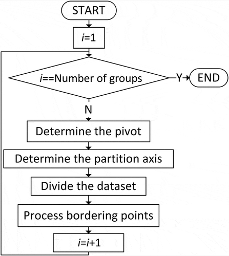
The partition algorithm proposed in this study is based on the k-d tree method, yet with a different tree construction strategy. There are two important steps in the tree construction process (Figure 1). The first is to select a pivot, which determines the data partition ratio between the left and right sub-trees. Some points may be exactly located along the splitting planes. The second step, then, is to develop a method to assign these points to subjacent sub-trees. These two steps are elaborated in the sections that follow.

Figure 1. A flow chart showing the data partition process.

2.1. The pivot values

This study used two different methods to determine the pivot values depending upon the total number (N) of data groups to be generated. Like the conventional k-d tree method, the median of data is used if N is a power of two. Otherwise, the pivot is set to ensure that the difference in layer numbers in the left and right sub-trees is no more than one to guarantee balanced workloads. In this study, the median was determined by the x and y coordinates of the point that ranks in the middle of the point dataset. Figure 2 shows the pseudo codes used to determine the pivot to partition the dataset into N groups.

Figure 2. The pseudo codes used to determine the partition pivot.

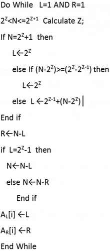
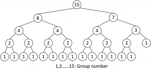
Where N is the total number of child data groups; Z is a positive integer; L and R are the numbers of layers in the left and right sub-trees, respectively; and A_L[i] and A_R[i] are the number of layers in the left and right sub-trees at level i, respectively. Figure 3 shows an example illustrating how the pseudo codes were used to determine the pivot values and construct the tree. The dataset was divided into 15 child data groups, which are represented by 15 leaf nodes. The whole dataset was first partitioned into two groups in the first level (Z = 2), with eight and seven child groups (nodes) on the left and right sub-trees, respectively. As the total number of nodes in the left sub-tree is a power of 2, it was further partitioned at its median. The right sub-tree was further partitioned using a pivot ratio of 4:3 to ensure that the maximum difference of layer numbers in the resulting left and right sub-trees is no more than one. The same procedure was utilized to further partition the sub-trees at the next level until the complete tree was constructed.

Figure 3. An example that illustrates how a k-d tree was constructed using different pivots at different levels to partition the whole dataset into 15 child data groups (nodes).

2.2. Points on the splitting planes

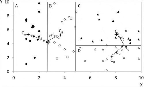
Some points may fall exactly on the splitting planes that partition the original dataset into different child data groups. This study used the distance to the mean centers of the child data groups to determine to which group the points should be assigned (Figure 4). In the example in Figure 4, point p is located exactly on the splitting plane that splits child data groups A and B. The distance from point p to the mean centers of groups A and B (C_A and C_B) was calculated. Point p was assigned to group B because d_B is less than d_A (Figure 4). A similar procedure was applied to point q, which is located on the splitting plane between groups C and D. Point q was assigned to group D as it is closer to its mean center. A point would be randomly assigned to one of the adjacent child data groups if its distance to the mean centers of these groups is exactly the same.

Figure 4. Points that are exactly on the splitting lines were assigned to a subgroup based on its distance to the mean centers (shown by stars) of the adjacent child data groups.

3. Experiment design

3.1. The study area and data

We tested the performance of our algorithm by partitioning a big sea surface temperature (SST) observation dataset in the South China sea (SCS) basin (Figure 5). The SCS is the largest semi-enclosed marginal sea in the northwest Pacific Ocean. Its total area is approximately 3.5 × 10⁶ km² with a mean depth of 1212 m. The SCS has a large NE–SW oriented abyssal basin with a greatest depth of 5567 m. The SCS is connected to the Pacific Ocean, the Sulu sea, the East China sea, and the Java sea through the Luzon strait, the Mindoro strait, the Taiwan strait, and the Karimata strait, respectively.

Figure 5. A map showing the study area and the SST observation data in the SCS.

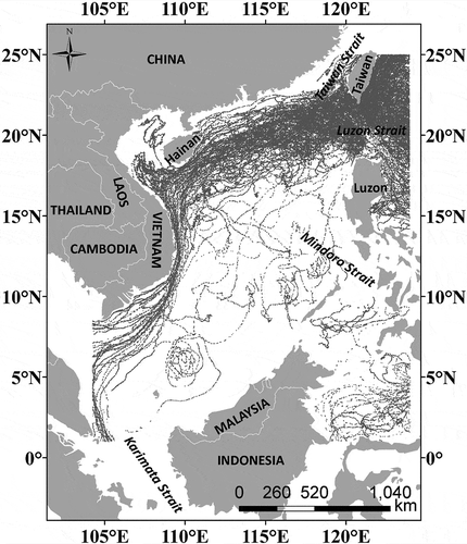
The SST dataset is recorded by Argo, which is a global array of more than 3000 free-drifting profiling floats that measure the upper water temperature and salinity in the ocean. A total of 3,27,546 data points were downloaded (ftp://www.usgodae.org/pub/outgoing/argo, http://www.meds-sdmm.dfo-mpo.gc.ca/isdm-gdsi/drib-bder/index-eng.htm, retrieved on 26 August 2014) for this study (Figure 5). We further prepared six datasets by randomly extracting different numbers of data points from the dataset (Table 1). These six datasets were used to evaluate the performance of our algorithm in data partitioning.

Table 1. Number of SST observations in the six sub-datasets.

Dataset	DS-1	DS-2	DS-3	DS-4	DS-5	DS-6
Points	327,546	265,894	212,488	122,479	113,219	71,372

3.2. Kriging interpolation

We then performed a parallel Kriging interpolation on the child data groups that were partitioned from the six datasets (Table 1). The Kriging method first creates the empirical semivariogram from the observation data to describe the spatial autocorrelation of the attribute to be interpolated (Burrough 1986). A model is used to fit the semivariogram and then predict the unknown values with minimum prediction errors, which are also estimated (Oliver and Webster 1990). The computational cost of Kriging interpolation significantly increases when it is applied to large datasets (Pesquer, Cortés, and Pons 2011). Therefore, it has been widely used to test the performance of parallel computing (e.g., Guan, Kyriakidis, and Goodchild 2011; Shi and Ye 2013; Shi et al. 2014).

Different strategies have been proposed to mitigate the computational costs associated with geostatistical simulations in Kriging interpolation. For instance, Tahmasebi et al. (2012) proposed a parallel fast simulation of spatial data based on graphics processing units (GPUs). Cheng (2013) used a compute unified device architecture (CUDA)-enabled GPU as a mathematical coprocessor to parallelize the universal Kriging algorithm on the NVIDIA CUDA platform. Cloud computing has recently emerged as a new approach to ad hoc parallel data processing (Dobre and Xhafa 2013).

In this study, the empirical semivariogram was first constructed from the SST datasets:

where h is the spatial distance between two measured points; N(h) is the total number of point pairs with a distance h; and and are the observation values (SST in this study) at points x_i and x_i+h (i = 1,2,…N(h)), respectively.

The spherical, exponential, and Gaussian functions are the three most widely used methods in Kriging interpolation. We evaluated the goodness of fit of these functions to the empirical semivariograms of our SST datasets, as well as their child data groups, using the standard errors of cross-validation and the coefficient of determination (R²) values (Healy 1984) between the predicated and actual values. A series of t-tests were performed, and no statistically significant difference was found between the goodness of fit of these three functions in fitting the empirical semivariograms. As a result, we chose the spherical function in this study for fitting the empirical semivariograms of our SST data.

Parameters of the spherical functions (range, sill, and nugget) were then determined from the empirical semivariograms. We first calculated the parameters from the empirical semivariograms of datasets DS-1 to DS-6, respectively, and those of the child data groups that were partitioned from a specified dataset. Hereafter, the former (Table 2) and latter (Table 3) parameters are referred to as global and local parameters, respectively. Both the global and local parameters were then optimized using the Levenberg–Marquardt algorithm (Madsen, Nielsen, and Tingleff 2004).

Table 2. The global parameters used to interpolate datasets DS-1 to DS-6.

Datasets	Nugget (m^2)	Range (m)	Partial sill (m^2)	Lag size (m)	Number of lags
DS-1	1.91	10,384.14	1.44	1298.02	12
DS-2	2.15	11,832.84	1.58	1479.11	12
DS-3	2.15	10,404.50	1.35	1300.56	12
DS-4	1.72	11,962.33	2.02	1495.29	12
DS-5	2.02	10,430.70	1.78	1303.84	12
DS-6	2.38	11,475.39	2.08	1434.42	12

Table 3. Examples of the local parameters used to interpolate child data groups.

Number of groups	Nugget (m^2)	Range (m)	Partial sill (m^2)	Lag size (m)	Number of lags
Dataset DS-1 was partitioned into 6 child data groups
1	0.38	21,466.72	0.90	2683.34	12
2	1.49	10,869.85	2.35	1358.73	12
…	…	…	…	…	…
6	2.27	10,903.88	0.74	1362.99	12
Dataset DS-3 was partitioned into 11 child data groups
1	1.03	11,514.13	1.23	1439.27	12
2	1.03	10,079.20	2.34	1259.90	12
…	…	…	…	…	…
11	2.42	9005.04	0.74	1125.63	12
Dataset DS-5 was partitioned into 5 child data groups
1	1.937	12,551.628	2.351	1568.954	12
2	2.447	9562.948	1.519	1195.368	12
…	…	…	…	…	…
5	1.731	12,564.171	1.216	1570.521	12

We then further evaluated whether the global or local parameters are more appropriate in parallel Kriging interpolation. For a specific child data group, the local parameters calculated from its empirical semivariogram and the global parameters calculated from the dataset from which the data group was partitioned were both used in the interpolation. The root mean square error (RMSE; Chai and Draxler 2014) was calculated by comparing the surfaces generated from the child data groups against the surface generated over the whole data. A t-test (0.458 > 0.05) was performed, and no statistically significant difference was found between the surfaces generated using the global parameters and the ones generated using the local parameters in terms of the RMSE values. Obviously, calculating the local parameters from each child data group would require more time, particularly when a dataset was partitioned into more child data groups. As a result, we used the global parameters in the parallel interpolation; the discussion hereafter is based on the surfaces generated using the global parameters unless otherwise specified.

3.3. Parallel computing framework

All experiments were conducted in a gigabit ethernet environment. We used two servers and four desktop computers with different hardware configurations (Table 4). Data partitioning and parallel Kriging interpolation were executed in a virtualized environment built with VMware Workstation v9.01. Computing nodes may change from 1 to 13 by either adding or deleting the virtual machines. A master/worker parallel framework was used in this study. The master node first reads the datasets; then their empirical semivariograms are built, from which the global parameters of the spherical function were calculated.

Table 4. Machine hardware configuration used in this study.

Machines	Number of machines	Number of cores	Core frequency	Internal memory
Intel Xeon	1	16	2.40 GHz	16 GB
Intel Xeon	1	16	2.40 GHz	12 GB
Intel Core i5-3470	4	4	3.20 GHz	4 GB

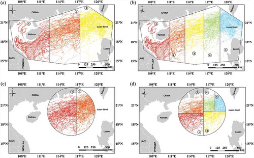
All datasets in Table 1 were, respectively, partitioned into 2 to 13 child data groups using our DPAKDT algorithm. All child data groups were indexed and assigned to individual worker nodes using the time slice round-robin method (Arpaci-Dusseau and Arpaci-Dusseau 2012). The local parameters of the spherical function were calculated from each child data group, and Kriging interpolation was then performed on individual worker nodes. Two or more spatially adjacent child data groups may be processed on the same work node. For this situation, surfaces generated from individual child data groups were stitched together on this worker node. In the end, surfaces generated on all worker nodes were spatially stitched together on the master node. The master node also monitored the progress of interpolation and stitching on each worker node.

3.4. Buffer zone settings and validation of interpolation results

A buffer zone was set for each child data group to ensure accurate interpolation results along the edges. Data points within the buffer zone were all considered in the calculation of the parameters of the spherical functions. In this study, we tested two different ways of determining an optimal buffer distance. The first method was to use the range of the global parameters in the spherical function (hereafter referred to as ‘global range’ unless otherwise specified) as the buffer distance for all its child data groups. The second was to use the range of the local parameters of each individual child dataset (hereafter referred to as ‘local range’ unless otherwise specified) as the buffer distance. Parallel Kriging interpolation was then performed on all 72 child data groups and the execution time was recorded to identify the optimal range for the interpolation.

A SST surface was also generated throughout our whole study area with all observation data using a similar Kriging interpolation method. The surface was compared against those produced from the parallel interpolation to evaluate influences of the buffer distance on the prediction accuracy/error. Such a comparison was also used to evaluate whether the process to stitch surfaces generated from individual child data groups influences the accuracy of the final output.

3.5. Data partitioning performance evaluation

Performance of our algorithm in partitioning data was evaluated using two methods. The first was to check whether it could evenly partition a big dataset to different child groups. All datasets in Table 1 were divided into 2 to 13 child groups. We counted and compared the number of points in each set of child data groups. The second method was to compare the data partitioning execution time against that of a conventional k-d tree method and two other partitioning algorithms. The conventional k-d tree algorithm first constructed a tree from all data points and then divided the tree into workload-balanced sub-trees. The spatial data partitioning algorithm based on decomposing hierarchy (SDPADH) first preliminarily partitioned a big dataset into child data groups using sparse Hilbert curves (Zhou, Zhu, and Zhang 2007). The resulting coarse grids were further adjusted using more Hilbert curves to ensure that all grids had the same data volume (workload). The spatial data partitioning algorithm based on grid (SDPAG) developed by Abugov (2004) partitioned big data using regularly spaced grids. This algorithm is able to quickly partition a big dataset, but it gives no consideration to workload balance. All three algorithms were programmed with the c# language and used to partition our SST datasets into the desired number of child data groups. Speed-up ratios of the execution time of our algorithm to that of the conventional k-d tree, the SDPADH, and the SDPAG algorithms were used to evaluate their performance in data partitioning.

3.6. Parallel interpolation performance evaluation

We then evaluated the performance of our algorithm in parallelizing Kriging interpolation. An interpolation of observation SST data in each child group was implemented on individual worker nodes. The execution time was recorded to evaluate workload balance and computing efficiency. Parallel interpolation was also performed on the child data groups that were generated using the SDPADH and the SDPAG algorithms. Speed-up ratios of the execution time of our algorithm to that of the SDPADH and the SDPAG were used to compare the influences of different partitioning algorithms on the performance of parallel Kriging interpolation.

4. Results and discussion

4.1. Evaluation of parallel interpolation results

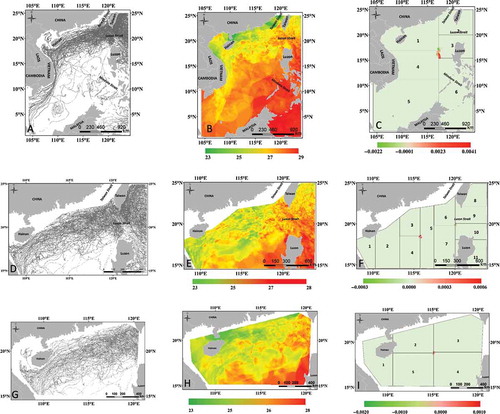
The parallel interpolation surfaces were first compared against the surface generated with the whole dataset. The surfaces are almost exactly the same, except for a few pixels along the splitting planes between adjacent child data groups. Figure 6 shows the comparison of the surfaces generated by parallel and sequential interpolation of datasets DS-1, DS-3, and DS-5. Figure 6C shows that different values were found at 892 pixels along the boundaries between child data groups 1, 3, 4, and 6 of dataset DS-1 when it was partitioned into six child groups. These pixels account for only 1.12% of the whole surface and the difference ranges only from −0.002 to 0.004 degrees. Figure 6F and I shows that the difference of surfaces generated from DS-3 (partitioned into 11 groups) and DS-5 (partitioned into 6 groups) ranges from −0.003 to 0.006 degrees and from −0.002 to 0.001 degree, respectively. The number of pixels with different predicted values account for only 0.25% and 0.09% of the whole surfaces of DS-3 and DS-5, respectively. There is no prominent discontinuity problem (Pesquer, Cortés, and Pons 2011) when the surfaces were generated using the global parameters. However, the problem is more prominent when the local parameters were used.

Figure 6. Comparison of parallel Kriging interpolation results against those produced by sequential Kriging interpolation results of the corresponding bulk datasets.

4.2. Performance in data partitioning

Our algorithm is fully capable of partitioning all datasets in Table 1 into the desired numbers of child data groups. Each child data group of the same dataset has almost the same number of points. Figure 7 shows the partitioning results of datasets DS-4 and DS-6 into different numbers of child groups. The DS-4 dataset was extracted from the bulk Argo data by an irregular polygon. As shown in Figure 7A, the polygon was partitioned into three different zones, with each zone representing one child data group. The zones have different areas yet contain almost exactly the same number of points. Zones 1 and 2 both have 40,826 points, whereas zone 3 has only one additional point. Dataset DS-4 was also partitioned into five child groups with an average point number of 24,495.8 and a standard deviation of 0.84 (Figure 7B). Points in dataset DS-6 were extracted from the bulk Argo data by a circle with a radius of 322 km. The dataset was partitioned into two child groups and each contains exactly 35,686 points (Figure 7C). The five child groups partitioned from dataset DS-6 have an average point number of 14,274.2 with a standard deviation of 0.84 (Figure 7D).

Figure 7. Partition results of datasets DS-4 and DS-6, which were extracted by a planar circle and an irregular polygon, respectively. DS-4 was partitioned into 3(A) and 5(B) groups. DS-6 was partitioned into 2(C) and 5(D) groups.

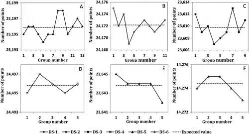
Figure 8 shows the number of points in each child data group, which were created from datasets DS-1 to DS-6 against the expectation values (the averages). The first three datasets were partitioned into 13, 11, and 9 child groups, whereas datasets DS-4 to DS-6 were all divided into five groups. All child groups from a specified dataset contain almost the same number of points with a very limited deviation from the averages. For example, when DS-2 was divided into 11 groups, the average number of points in each child group is 24,172. Partition results show that the actual number of points in the groups is very close to the average. The maximum deviation was found in the first and fourth groups, which have three points more and less than the average, respectively. Table 5 lists the average and deviation of the number of points in the child data groups that were created by dividing dataset DS1 into 2–13 groups. The maximum deviation is 7 when dataset DS-1 was divided into 12 groups, and the minimum deviation of 1 was found when it was divided into two groups. We further randomly selected 32 out of all our 72 child data groups and performed a two-tail t-test. The results (t = 2.571 > 0.4, P > 0.05 at a significance level of 0.95) show that there is no statistically significant difference between the actual numbers of points and the corresponding averages in each partition scenario.

Table 5. Parallel interpolation execution time of dataset DS-1, which was partitioned into 2 to 13 child data groups.

Numbers of group	Partition time (ms)	Number of points in each child group		Interpolation time (ms)		Distribution, emergence time (ms)	Total (ms)
		Average	Std.	Average	Std.
2	2123	163,773.00	1.40	259,865.50	4.95	9769	2,710,761
3	2141	109,182.00	2.60	221,658.70	2.52	16,297	245,099
4	2159	81,886.50	1.70	158,204.50	3.87	27,265	187,633
5	2175	65,509.20	2.80	123,346.20	5.97	32,618	158,147
6	2186	54,591.00	2.00	103,629.80	6.74	40,812	146,627
7	2195	46,792.29	2.80	85,567.14	5.46	96,755	184,505
8	2212	40,943.25	2.70	74,715.88	5.74	118,456	195,359
9	2225	36,394.00	3.00	66,675.11	7.62	152,543	221,406
10	2236	32,754.60	3.30	59,010.20	6.80	176,027	237,221
11	2248	29,776.91	2.90	52,240.00	7.82	209,145	263,579
12	2259	27,295.50	4.30	47,526.83	9.29	273,497	323,221
13	2268	25,195.69	1.30	43,022.38	10.11	334,335	379,554

Figure 8. Comparison of the actual number of points in each child data group against the corresponding expectation values.

Speed-up ratios of data partitioning execution times between our algorithm and the conventional k-d tree, the SDPADH, and the SDPAG algorithms were calculated, respectively, to further evaluate the performance of our algorithm in data partitioning (Figure 9). The speed-up ratios of our algorithm compared to the conventional k-d tree are always much higher than one (Figure 9A), indicating that our partition algorithm significantly outperforms the conventional k-d tree algorithm in data partitioning. Figure 9A also shows that the speed-up ratios increased significantly with an increasing data amount but dropped with an increase in the number of child data groups. For example, the average ratio increased from 17.11 of dataset DS-6 to 26.68 of DS-1. These two datasets have 71,372 and 327,546 points respectively. The speed-up ratio of DS-1 dropped from 30.23 to 25.68 when the numbers of child data groups increased from 5 to 10.

Figure 9. Data partitioning performance evaluation results of our algorithm as shown by speed-up ratios of execution time between our algorithm and the conventional k-d tree (7A). (B) and (C) The speed-up ratios of execution time of the SDPADH, the SDPAG, and our algorithm, respectively.

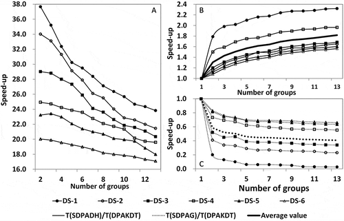
Figure 9B and C shows the speed-up ratios of partitioning time of the SDPADH/SDPAG and our algorithm, respectively. For all datasets, the T_SDPADH/T_DPAKDT speed-up ratios and the average are always lower than one, whereas the T_SDPAG/T_DPAKDT ratios are higher than one. In other words, our algorithm significantly outperforms the SDPADH, particularly in partitioning a bigger dataset (Figure 9C). For example, the speed-up ratios are about 0.25 and 0.65 when the SDPADH and our algorithms were used to divide datasets DS-2 and DS-5 into more than 6 groups. However, our algorithm is not as efficient as the SDPAG in data partitioning, particularly when a dataset was partitioned into more child groups, as shown by a gradual increase in the speed-up ratios with an increasing number of child data groups. However, the SDPAG tends to oversimplify the data partitioning process without any guarantee of balanced workloads, as further illustrated in the following section.

4.3. Performance in parallel interpolation

Our algorithm also shows outstanding performance in parallel Kriging interpolation. Table 5 shows its execution time in parallel Kriging interpolation of the child data groups that were generated from dataset DS-1. As mentioned in the previous section, our algorithm is able to evenly divide the dataset into the desired number of child groups. There is no significant difference in partitioning execution time (usually around 2200 ms), no matter how many child data groups the dataset DS-1 was partitioned into. The average interpolation time dropped significantly with an increased number of child groups. The standard deviation of interpolation time is insignificant compared with the averages. The distribution and emergence time significantly increased when the parallel interpolation was performed in more child data groups. It took more time to stitch together the interpolated surfaces produced on individual worker nodes. The total execution time gradually dropped when dataset DS-1 was partitioned into more groups. It reached its minimum when the dataset was divided into six groups. After that, the execution time increased quickly when the dataset was divided into more child groups. Exactly the same variation patterns were also observed on the variations of execution times for datasets DS-2 to DS-6 and thus were not presented in this section.

Figure 10A–C shows speed-up ratios of parallel interpolation execution time of our algorithm, the SDPADH, and the SDPAG in relation to that of the sequential interpolation. With an increase in the total number of groups, the speed-up ratios gradually increased and then dropped after they reached their maxima when the datasets were divided into four to seven child groups. The speed-up ratios became higher when the algorithms were applied to interpolate bigger datasets. For instance, the DPAKDT achieved an average speed-up ratio of 2.78 when it was applied to interpolate the DS-1 dataset. It dropped to 2.11 for DS-6, which has significantly fewer data points than DS-1 (Table 2). Therefore, the DPAKDT shows some advantages in parallelizing the Kriging interpolation of large datasets. For a specific dataset, the speed-up ratios gradually increased when the dataset was partitioned into more child data groups. The algorithms usually achieved their maximum speed-up ratios when the datasets were divided into four to six groups. The ratios significantly dropped when the datasets were divided into more groups.

Figure 10. Comparison of execution time of parallel versus sequential interpolation: (A) DPAKDT, (B) SDPADH, (C) SDPAG, and (D) average of speed-up ratios of all datasets.

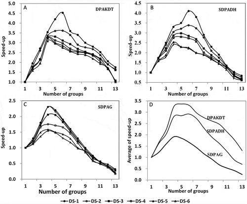
It is also interesting to note that our algorithm always outperforms the sequential interpolation regardless of the number of data points in a specific dataset and the number of child groups the datasets were divided into. For the SDPADH and ADPAG algorithms, speed-up ratios dropped to less than one when the datasets were partitioned into more than 11 and 8 child groups, respectively (Figure 10B–C), indicating poorer computing performance than the sequential interpolation. In particular, the speed-up ratios of the SDPADH and the SDPAG dropped to ~0.84 and 0.32, respectively, when the datasets were divided into 13 groups. Such low speed-up ratios are mainly due to unbalanced workloads assigned to individual worker nodes. As a result, achieving higher performance of parallel computing requires an optimal number of subgroups that a dataset should be divided into and balanced workloads assigned to each worker node. In general, our algorithm outperforms the other two algorithms in terms of dividing the datasets into the optimal number of child groups and ensuring balanced workloads assigned to individual worker nodes. It can achieve a maximum average speed-up ratio of 4.53, which is significantly higher than that of the SDPADH (4.1) and SDPAG (2.3) (Figure 10D).

5. Conclusions

Unevenly distributed spatial data pose a challenge to data partitioning in parallel computing. We proposed a new algorithm, DPAKDT, to optimize the data partition process in this research. Although it is based on the conventional k-d tree data structure, the DPAKDT is able to build a tree with a number of final sub-trees that are not always a power of two. The algorithm also created balanced left and right sub-trees, of which the difference between their leaf nodes is always no more than one. Such a workload-balanced tree structure ensures balanced workloads on individual worker nodes in parallel computing.

The performance of the DPAKDT was tested using six different datasets. The algorithm was also compared against two other data partition algorithms (SDPADH and SDPAG) in terms of their performance in data partitioning and creating a balanced workload on individual worker nodes. The results show that with an increase in the data amount and number of groups, the DPAKDT shows significantly higher speed-up ratios in data partitioning than the SDPADH. The DPAKDT also shows more efficiency in parallel Kriging interpolation than the sequential interpolation.

Data parallelism is one efficient way to handle large spatial data. However, special algorithms are needed to partition spatial data, which tend to be spatially auto-correlated. Such algorithms need to further consider the characteristics of spatial data and for what applications parallel computing is used. The algorithm we proposed in this study is able to partition unevenly distributed point data into workload-balanced child groups. For a specified dataset, there is no statistically significant difference in the interpolation results derived from different Kriging models. For the child data groups partitioned from a specified dataset, there is also no statistically significant difference in the interpolation results derived using the global and local parameters in the spherical semivariogram model. There is a slight difference between the surfaces generated from the parallel Kriging interpolation of child data groups compared to those derived from the whole dataset. The difference is mainly found along the boundaries of child data groups. However, setting up an optimal buffer zone for the interpolation successfully minimized the difference and ensured the accuracy of parallel interpolation results. For other applications, such as delineating watersheds from high spatial resolution digital elevation data, it is more challenging to partition large datasets into workload-balanced groups while ensuring that elevation points contributing to one watershed are partitioned into the same group or stitched together after parallel computing. Further studies are needed to meet such challenges in spatial data parallel computing.

Disclosure statement

No potential conflict of interest was reported by the authors.

Acknowledgment

The authors thank the anonymous reviewers for their constructive comments, which have helped to improve the manuscript significantly.

Additional information

Funding

This work was supported by the Oceanic Department Public Benefit Research Foundation [grant number 201105033], [grant number 201105017].

References

- Abel, D. J., and D. M. Mark. 1990. “A Comparative Analysis of Some Two-Dimensional Orderings.” International Journal of Geographical Information Systems 4 (1): 21–31. doi:10.1080/02693799008941526.
- Abugov, D. 2004. Oracle Spatial Partitioning: Best Practices (an Oracle White Paper). Redwood Shores, CA: Oracle Inc.
- Al-Furajh, I., S. Aluru, S. Goil, and S. Ranka. 2000. “Parallel Construction of Multidimensional Binary Search Trees.” IEEE Transactions on Parallel and Distributed Systems 11 (2): 136–148. doi:10.1109/71.841750.
- Armstrong, M. P. 2000. “Geography and Computational Science.” Annals of the Association of American Geographers 90 (1): 146–156. doi:10.1111/0004-5608.00190.
- Arpaci-Dusseau, R. H., and A. C. Arpaci-Dusseau. 2012. “Scheduling Introduction.” In Operating Systems: Three Easy Pieces, Arpaci-Dusseau Books, 7–8, University of Wisconsin: Madison.
- Bentley, J. L. 1975. “Multidimensional Binary Search Trees Used for Associative Searching.” Communications of the ACM 18 (9): 509–517. doi:10.1145/361002.361007.
- Brinkhoff, T., H. P. Kriegel, and B. Seeger. 1996. “Parallel Processing of Spatial Joins Using R-Trees.” In Proceedings of the Twelfth International Conference on Data Engineering, February 258–265. New Orleans, LA: IEEE.
- Burrough, P. A. 1986. Principles of Geographical Information Systems for Land Resources Assessment, 193. Oxford: Oxford University Press.
- Chai, T., and R. R. Draxler. 2014. “Root Mean Square Error (RMSE) or Mean Absolute Error (MAE)?-Arguments Against Avoiding RMSE in the Literature.” Geoscientific Model Development 7: 1247–1250. doi:10.5194/gmd-7-1247-2014.
- Cheng, T. 2013. “Accelerating Universal Kriging Interpolation Algorithm Using CUDA-Enabled GPU.” Computers & Geosciences 54: 178–183. doi:10.1016/j.cageo.2012.11.013.
- Choi, B., R. Komuravelli, V. Lu, H. Sung, R. L. Bocchino, S. V. Adve, and J. C. Hart. 2010. “Parallel SAH K-D Tree Construction.” In Proceedings of the Conference on High Performance Graphics, Switzerland, June 77–86.
- Clematis, A., M. Mineter, and R. Marciano. 2003. “High Performance Computing with Geographical Data.” Parallel Computing 29 (10): 1275–1279. doi:10.1016/j.parco.2003.07.001.
- Dobre, C., and F. Xhafa. 2013. “Parallel Programming Paradigms and Frameworks in Big Data Era.” International Journal of Parallel Programming 42 (5): 701–738. doi:10.1007/s10766-013-0272-7.
- Farber, R. 2012. “Data and Task Parallelism.” In CUDA Application Design and Development, Robyn Day, 18–19, San Francisco: Morgan Kaufmann.
- Filippi, A. M., B. L. Bhaduri, T. Naughton, A. L. King, S. L. Scott, and I. Güneralp. 2012. “Hyperspectral Aquatic Radiative Transfer Modeling Using a High-Performance Cluster Computing-Based Approach.” GIScience & Remote Sensing 49 (2): 275–298. doi:10.2747/1548-1603.49.2.275.
- Guan, Q., and K. C. Clarke. 2010. “A General-Purpose Parallel Raster Processing Programming Library Test Application Using a Geographic Cellular Automata Model.” International Journal of Geographical Information Science 24 (5): 695–722. doi:10.1080/13658810902984228.
- Guan, Q., P. C. Kyriakidis, and M. F. Goodchild. 2011. “A Parallel Computing Approach to Fast Geostatistical Areal Interpolation.” International Journal of Geographical Information Science 25 (8): 1241–1267. doi:10.1080/13658816.2011.563744.
- Hawick, K. A., P. D. Coddington, and H. A. James. 2003. “Distributed Frameworks and Parallel Algorithms for Processing Large-Scale Geographic Data.” Parallel Computing 29 (10): 1297–1333. doi:10.1016/j.parco.2003.04.001.
- Healy, M. J. R. 1984. “The Use of R2 as a Measure of Goodness of Fit.” Journal of the Royal Statistical Society 147 (4): 608–609. doi:10.2307/2981848.
- Henrich, A., H. W. Six, F. Hagen, and P. Widmayer. 1989. “The LSD-Tree: Spatial Access to Multidimensional Point and Non-Point Objects.” In Proceedings of the 15th International Conference on Very Large Data Bases, San Francisco, July 45–53.
- Kamel, I., and C. Faloutsos. 1994. “Hilbert R-tree: An Improved R-Tree Using Fractals.” In Proceedings of the 20th International Conference on Very Large Data Bases, San Francisco, September 500–509.
- Madsen, K., H. B. Nielsen, and O. Tingleff. 2004. “The Levenberg–Marquardt Method.” In Methods for Non-Linear Least Squares Problems, 24–29. Lyngby: Informatics and Mathematical Modelling. Technical University of Denmark.
- Oliver, M. A., and R. Webster. 1990. “Kriging: A Method of Interpolation for Geographical Information Systems.” International Journal of Geographical Information Systems 4 (3): 313–332. doi:10.1080/02693799008941549.
- Pesquer, L., A. Cortés, and X. Pons. 2011. “Parallel Ordinary Kriging Interpolation Incorporating Automatic Variogram Fitting.” Computers & Geosciences 37 (4): 464–473. doi:10.1016/j.cageo.2010.10.010.
- Samet, H. 1980. “Region Representation: Quadtrees from Binary Arrays.” Computer Graphics and Image Processing 13 (1): 88–93. doi:10.1016/0146-664X(80)90118-5.
- Samet, H. 1982. “Neighbor Finding Techniques for Images Represented by Quadtrees.” Computer Graphics and Image Processing 18 (1): 37–57. doi:10.1016/0146-664X(82)90098-3.
- Shi, X., M. Huang, H. You, C. Lai, and Z. Chen. 2014. “Unsupervised Image Classification over Supercomputers Kraken, Keeneland and Beacon.” GIScience & Remote Sensing 51 (3): 321–338. doi:10.1080/15481603.2014.920229.
- Shi, X., and F. Ye. 2013. “Kriging Interpolation over Heterogeneous Computer Architectures and Systems.” GIScience & Remote Sensing 50 (2): 196–211. doi:10.1080/15481603.2013.793480.
- Tahmasebi, P., M. Sahimi, G. Mariethoz, and A. Hezarkhani. 2012. “Accelerating Geostatistical Simulations Using Graphics Processing Units (GPU).” Computers & Geosciences 46: 51–59. doi:10.1016/j.cageo.2012.03.028.
- Turton, I., and S. Openshaw. 1998. “High-Performance Computing and Geography: Developments, Issues, and Case Studies.” Environment and Planning A 30 (10): 1839–1856. doi:10.1068/a301839.
- Wald, I., and V. Havran. 2006. “On Building Fast KD-Trees for Ray Tracing, and on Doing That in O (N log N).” In IEEE Symposium on Interactive Ray Tracing, Salt Lake City, September 61–69. doi:10.1109/RT.2006.280216.
- Wang, S., and M. P. Armstrong. 2003. “A Quadtree Approach to Domain Decomposition for Spatial Interpolation in Grid Computing Environments.” Parallel Computing 29 (10): 1481–1504. doi:10.1016/j.parco.2003.04.003.
- Wu, W., Y. Rui, F. Su, L. Cheng, and J. Wang. 2014. “Novel Parallel Algorithm for Constructing Delaunay Triangulation Based on a Twofold-Divide-and-Conquer Scheme.” GIScience & Remote Sensing 51 (5): 537–554. doi:10.1080/15481603.2014.946666.
- Yin, L., S.-L Shaw, D. Wang, E. A. Carr, M. W. Berry, L. J. Gross, and E. J. Comiskey. 2012. “A Framework of Integrating GIS and Parallel Computing for Spatial Control Problems - a Case Study of Wildfire Control.” International Journal of Geographical Information Science 26 (4): 621–641. doi:10.1080/13658816.2011.609487.
- Zhou, Y., Q. Zhu, and Y. T. Zhang. 2007. “A Spatial Data Partitioning Algorithm Based on Spatial Hierarchical Decomposition Method of Hilbert Space-Filling Curve.” Geography and Geo-Information Science 4 5. doi:10.11834/jig.20131016.