Extracting buildings from airborne laser scanning point clouds using a marked point process

Abstract

Automatic extraction of buildings from airborne laser scanning (ALS) point clouds is essential for 3D building reconstruction. This paper presents a two-part approach for extracting buildings from ALS data. First, building objects are extracted from ALS data by a marked point process using the Gibbs energy model of buildings and sampled by a reversible jump Markov chain Monte Carlo algorithm. Second, a refinement operation is performed to filter the non-building points and false building objects before extracting buildings from the detected building objects. Experimental results and evaluation using ISPRS benchmark data-sets showed the robustness of the proposed method.

Keywords:

• building extraction
• marked point process
• airborne laser scanning
• point clouds filtering

1. Introduction

Data for building outlines are an invaluable data source for automatic generation of cadastral maps, 3D building reconstructions, change detection and so on. Airborne laser scanning (ALS) systems have become an accepted means of capturing accurate spatial data because of their short data acquisition and processing times, relatively high accuracy and point density, and low acquisition costs (Brennan and Webster 2006; Yang et al. 2012). ALS data have been widely used for many applications such as man-made objects detection, trees detection and forest CO₂ storage (e.g. Brenner 2005; Lee, Kim, and Choi 2013). Various approaches for extracting buildings have been reported in the last decade (e.g. Brenner 2005).

One solution is first to resample ALS data into grids and then to extract buildings using image processing methods (e.g. planar detection) (Alharthy and Bethel 2002; Rottensteiner and Briese 2002; Lodha, Fitzpatrick, and Helmbold 2007; Meng, Wang, and Currit 2009; Lu, Im, and Quackenbush 2011; Yang, Wei, et al. 2013). Nevertheless, the gridding of ALS data involves the loss of information and accuracy in building detection. Miliaresis and Kokkas (2007) extracted buildings from a digital surface modelling (DSM)-guided image according to geomorphometric segmentation principles. The extracted results depended on the seed cells and region-growing criteria specified. Approaches that use segmentation to distinguish building objects from ALS data have also been reported in recent years. Im, Jensen, and Hodgson (2008) classified high-posting-density LiDAR data by machine-learning decision trees based on eight object-based metrics. But most of the classification errors were found along the boundaries between objects, such as the boundary between a building and a road. Poullis and You (2009) presented processes to reconstruct simplified building models of urban areas where the input point clouds are segmented as regularized buildings or building parts. Niemeyer, Rottensteiner, and Soergel (2013) used a supervised classification of ALS points based on conditional random fields which incorporated a statistical context model (Niemeyer et al. 2011). To obtain binary object masks for both classes, the resulting point clusters for each class were projected into a label image, which finally was smoothed by morphological operations. The classification results provided beneficial sources for building detection. Lafarge and Mallet (2012) presented a solution for reconstructing buildings, trees and topologically complex grounds from ALS data by incorporating an unsupervised method and template fitting of geometric primitives. Henn et al. (2013) reconstructed 3D building models from ALS data and building footprints using random sample consensus (RANSAC) and support vector machine (SVM) methods. Nevertheless, the segmentation of relatively small roof structures and accurate determination of roof edges are always difficult (Huang, Brenner, and Sester 2013).

Another solution is to extract building objects by fusing ALS data and auxiliary data (e.g. aerial imagery, 2D maps) (Cheng et al. 2011; Sohn and Dowman 2007; Vosselman and Dijkman 2001). Bartels and Wei (2006) performed pixel-based classification of ALS data and aerial imagery using the Bayesian maximum-likelihood approach. Rottensteiner et al. (2004) and Lu, Trinder, and Kubik (2006) extracted buildings from ALS data and aerial imagery based on the Dempster–Shafer theory. Moussa and El-Sheimy (2012) classified ALS data into building, tree and ground segments using rule-based segmentation and classification by combining ALS data with an ortho-rectified colour infrared image. With the help of auxiliary data, building extraction performance can be improved. However, up-to-date auxiliary data (e.g. imagery) are not always available, and registration with point clouds is still a non-trivial issue.

The marked point process has been widely used to extract objects from high-resolution imagery because approaches that use marked point processes do not require initial information (e.g. plane detection, localization information, number of buildings) for object extraction. Stoica, Descombes, and Zerubia (2004) proposed a marked point process approach to detect road networks from remotely sensed images. Perrin, Descombes, and Zerubia (2005a) presented a stochastic geometry approach to extract 2D and 3D parameters of trees from remotely sensed imagery by modelling the stands as realizations of a marked point process involving ellipses and ellipsoids. However, this approach required conversion of remotely sensed imagery into binary images. Ortner, Descombes, and Zerubia (2007) and Tournaire et al. (2010) presented methods to extract buildings from high-resolution digital evaluation methods (DEMs) in urban areas using a marked point process. The Ortner energy model requires many parameters to be tuned simultaneously, leading to heavy computational costs and time complexity. On the other hand, the data-coherence energy term of Tournaire et al. (2010) was calculated using the average gradient of each edge of building roof outlines. Nevertheless, the extraction result was poor when the boundaries of building were not obvious or when buildings were close to each other. Tournaire and Paparoditis (2009) proposed a marked point process–based approach to detect the dashed lines of road markings from very high-resolution aerial images. Lafarge, Gimel’farb, and Descombes (2010) presented a multi-marked point process for extracting multiple kinds of objects (e.g. linear objects, areal objects) from images. Huang, Brenner, and Sester (2013) presented processes to reconstruct building roofs using a reversible jump Markov chain Monte Carlo (RJMCMC) strategy to search roofs according to a predefined library of roof primitives. The reconstruction results reported by Huang, Brenner, and Sester (2013) are promising, although the completeness of the reconstruction is influenced by the predefined library of roof primitives and the scene complexity.

The high density of urban areas and the complexity of man-made objects make the building extraction process difficult to perform successfully. Although reported building detection methods have achieved considerable progress, the robustness and omission errors of existing methods still need to be improved. This paper presents a marked point process method for extracting buildings from ALS point clouds by improving and extending the work of Yang, Xu, and Dong (2013). The proposed method aims to detect buildings from large urban scenes with an unknown number of buildings of various sizes and shapes. The main differences from the work of Yang, Xu, and Dong (2013) are two folders: (1) the energy model of building objects is modelled to fit the building points by isolating building façade points, particularly for small buildings (e.g. shacks) and (2) a refinement operation is integrated to discard trees like objects and to detect the buildings without flat roofs, resulting in the completeness improvement in building detection. The proposed method consists of three key steps. First, the Gibbs energy model of building objects is fitted to the building shapes (data-coherence term) and the spatial relationships between buildings (prior-constraint term). Then, RJMCMC coupled with simulated annealing is used to find a maximum a posteriori estimate of the number, locations and sizes of building objects from the Markov chain made up of the Gibbs energy model of the building objects. Finally, a refinement operator is used to extract buildings from the identified building objects by filtering out false buildings and merging connecting parts of buildings.

Following the Introduction, Section 2 elaborates upon the proposed building object detection method. Section 3 provides details of the extraction of building roof outlines. Section 4 presents the results for the benchmark data-set provided by ISPRS and compares the results of the proposed method with those of Yang, Xu, and Dong (2013). Concluding remarks are then provided in Section 5. Figure 1 shows the flow chart of our method.

Figure 1. The flow chart of building extraction based on marked point process.

2. Detecting buildings using a marked point process

The method presented here is based on a marked point process and generates a cuboid layout representing the building objects. A marked point process is an object-oriented statistical geometrical method. Complex marked point processes introduce both consistent measurements within data and interactions between objects that can be defined by specifying a density with respect to the distribution of a reference Poisson process (Lafarge, Gimel’farb, and Descombes 2010). The proposed method is well adapted to this problem because it describes buildings with complex shapes and diverse forms as simple cuboids, enables the use of prior knowledge of building layout and does not require any initialization (e.g. location, size). Each building is described by an energy model associated with a configuration. The global minimum of the energy model is then found by applying an RJMCMC strategy sampler coupled with a simulated annealing scheme (Green 1995). Finally, a refining process is used to achieve further improvements in the quality of the building set detected.

2.1. Marked point process

Let be a marked point process in data space . Each object of is defined by its position in a data space and its mark in a marked space . Generally, the position corresponds to the centre of the object. is a measurable mapping from a probability space to configurations of points of , in other words a random variable whose realizations are random configurations of objects (Perrin, Descombes, and Zerubia 2005b). The process of building extraction from an ALS data space can be regarded as a Poisson process, which is a kind of spatial stochastic point process. More details on Poisson processes can be found in Yang, Xu, and Dong (2013). The marked space consists of a marked point process of cuboids that are defined to describe buildings. The associated set space can be described as

(1)

where , and are the centre coordinates of a cuboid, , and are the length, width and height of the cuboid, respectively, and is the orientation of the cuboid in the X–Y plane. Each cuboid represents a building object as described by the Gibbs energy model.

2.2. Gibbs energy model of buildings

Let us consider a marked point process defined through its probability density with respect to the law of a Poisson process known as the reference process. can be defined through a Gibbs energy . Thus, the density of a configuration can be written as in Equation (2):

(2)

where is a normalizing constant, , is the configuration space of the objects, and configuration contains a series of objects. Moreover, the Gibbs energy can be expressed as a sum of a data-coherence energy term , which represents the quality of the objects (external energy), and a prior-constraint energy , which measures the spatial quality of the collection of objects (prior or internal energy). The Gibbs energy can be written as:

(3)

2.2.1. Data-coherence term for buildings

The data-coherence energy term measures the quality of the match between building objects and ALS data. can be decomposed into the sum of the local energy related to each object of configuration :

(4)

where is a measure of the coherence of building object with respect to ALS data, and is the number of objects in configuration As far as building objects are concerned, the inside region (roof) elevation of one building is relatively consistent, and a large elevation difference occurs between the inside and outside regions. The inside region of a particular building object is the envelope region of the building outline. The outside region of one building is formed by expanding the inside region outward over a certain width ranging from 1 to 3 m in practice. The Mahalanobis distance was used in the Gibbs energy model of buildings because it is a useful way of determining the similarity of two unknown sample sets. It differs from Euclidean distance in that it takes into account the correlations in the data-set and is scale-invariant (Yang, Xu, and Dong 2013). can be written as:

(5)

where is the Mahalanobis distance between the inside and outside regions of one cuboid, and are the mean elevations of the ALS points in the inside and outside regions of the cuboid, and are the standard deviations of the elevations of ALS points in the inside and outside regions of the cuboid, and and are the numbers of ALS points in the inside and outside regions of the cuboid. The threshold makes it possible to tune the data-fitting sensitivity. When the cuboids match well with the building objects in the ALS data, a highly negative data-coherence energy term is obtained.

The façade points of buildings have a large effect on the elevation difference between the inside and outside regions of small buildings (e.g. low buildings) and should be excluded from the calculation of the data-coherence energy term. The normal vectors of the points in the cuboid are estimated by decomposing the local covariance matrix of each point, which is formatted using its neighbouring points in the corresponding region according to principal component analysis (PCA). The angle between the normal vector of each point and the Z-direction is then calculated to eliminate façade points. In practice, if the angle between the normal vector of one point and the Z-direction is > 75°, the point is marked as a façade point and excluded from the calculation of the data-coherence energy term. This step is beneficial for performing accurate data-coherence energy term calculations for small buildings.

2.2.2. Prior-constraint term for buildings

introduces prior knowledge of buildings by taking into account pairwise interactions between buildings, strong structural constraints, edge gradients of buildings and fill percentages of points in cuboids. The prior energy associated with buildings can be described as:

(6)

The prior-knowledge or penalty term embodies the overlapping relationship between buildings and penalizes overlapping buildings. The larger the overlap, the larger will be the penalty. To avoid too much overlap, the overlapping threshold is empirically specified as 0.1. If the overlapping volume between cuboids is greater than this threshold, an infinite energy is specified. The calculation of the penalty term between two overlapping buildings can be written as

(7)

where and are the building objects in configuration , is a penalty term between buildings and , and are the volumes of and , respectively, and is the volume of the overlapping part of and .

To prevent extreme closeness between the detected cuboids, an infinite energy is assigned to pairs of too close objects. This is to avoid marking one area with multiple marks. A distance threshold is specified to control the minimum distance between the centre points of the cuboids. In this research, was set to 3 m for extracting buildings, which means that the maximum width of the overlap between two cuboid outlines should be greater than 3 m:

(8)

where is the width of the overlap between the outlines of cuboid and cuboid .

On the other hand, a gradient constraint for building roof outlines was added to the prior-knowledge term for buildings. The gradient of a point is calculated as the maximum value of the height differences between that point and its neighbouring points. The neighbouring points of one point are searched within a radius equal to the average point spacing. If no points are searched, the gradient value of the point is set to zero. The gradient of each edge of a cuboid is set to the average gradients of the points along the edge. Suppose that the gradient of a cuboid edge is less than a threshold. The cuboid will be assigned a penalty factor, which is written as

(9)

where is the number of the edge having a gradient less than the threshold. The gradient threshold is specified as 1.0, indicating that the minimum height between building roof points and neighbouring points (e.g. ground points, vegetation points) should be greater than 1.0 m.

For a discrete random distribution of ALS data, it is hard to guarantee that each cuboid has enough roof points in it. Hence, the fill percentage of a cuboid was defined as the number of points in each cuboid divided by the area enclosed by the cuboid outline. The prior term associated with the fill factor of each cuboid is calculated as:

(10)

Equation (10) indicates that if the fill percentage of a cuboid is less than 0.5/m², the cuboid constitutes a poor match to the potential building objects in the ALS data, and an infinite energy is therefore assigned.

2.3. Finding the minimum Gibbs energy

The minimum energy of must then be found to achieve the optimal match between building objects and their corresponding ALS data. An RJMCMC sampler algorithm coupled with a simulated annealing optimization method is particularly well adapted to obtaining the global minimum solution of the Gibbs energy (Lafarge et al. 2008; Tournaire and Paparoditis 2009). This solution effectively overcomes the shortcomings of traditional methods, which could find only a local minimum solution.

2.3.1. The RJMCMC algorithm

The Markov chain Monte Carlo (MCMC) algorithm is a simple and effective Bayesian calculation method. This iterative algorithm does not depend on the initial state. Green (1995) proposed a RJMCMC method, which is a special Metropolis–Hastings method which can reversibly jump between the different subspaces. The jump probability is determined by the Green’s ratio, which ensures the reversibility of the Markov chain. RJMCMC makes it possible to build a new configuration from a random starting configuration by modifying an already existing object or by adding or removing an object from the current configuration, thus involving a change in the dimension space. Reversible jumps between the different subspaces are performed according to the families of moves called proposition kernels. Each proposition kernel is associated with a different Green’s ratio. For each proposition kernel used in this paper, the Green’s ratio computation can be found in Green (1995), Perrin, Descombes, and Zerubia (2005b) and Lafarge, Gimel’farb, and Descombes (2010).

The proposition kernels contain birth, death, translation, rotation, dilation, split and merge operations that have been proven effective for the convergence of the Markov chain (Tournaire and Paparoditis 2009). To obtain the minimum solution rapidly, the various proposition kernels should be endowed with different selection probabilities. The translation, rotation and dilation proposition kernels are generally endowed with a high probability in applications (Perrin, Descombes, and Zerubia 2005a). In our study, the probabilities of the proposition kernels for birth, death, translation, rotation, dilation, split and merge were assigned as 0.1, 0.1, 0.2, 0.2, 0.2, 0.1 and 0.1, respectively.

The birth and death proposition kernels serve to add an object to the current configuration with a given probability or to remove an object from the current configuration with a given probability. This research has assumed that objects with higher data-coherence energy are chosen first to perform death proposition kernel processing. The translation, rotation and dilation proposition kernels do not change the number of objects, but rather modify the parameters of the chosen objects. Moreover, the transformation type and objects are chosen randomly. This guarantees quick convergence and a finer position adjustment at the end of the process until all objects are detected. The split and merge proposition kernels are used to avoid under-detection or over-detection of objects.

2.3.2. Simulated annealing

Some local search algorithms (e.g. the gradient descent method) are prone to getting stuck in local minima. The RJMCMC sampler is coupled with a simulated annealing algorithm to find the minimum global value of the Gibbs energy . The density function is replaced by the function , where is a decreasing sequence of temperatures which tends to zero as becomes infinitesimal (Tournaire and Paparoditis 2009). Then, the density function can be expressed as:

(11)

This ensures convergence to the global optimum from any initial configuration using a logarithmic decrease in temperature. In practice, it is impossible to use such a cooling approach because the algorithm has a long running time. Hence, a geometric temperature decrease is used in the simulated annealing algorithm to obtain a good solution close to the minimum. The cooling formula can be written as:

(12)

where is the initial temperature, is a coefficient of decrease which is close to, but less than 1, and is the time of the temperature decrease. The coefficient of decrease can be modified according to variations in energy. However, the time savings are usually relatively minor in practice. This is why a constant coefficient of decrease is generally used in the simulated annealing algorithm (Lafarge, Gimel’farb, and Descombes 2010). During the cooling procedure, the temperature cools by one unit for every iterations. The purpose of this is to make the energy reach balance at every single temperature. The energy of each building object is recorded and tracked during each iteration. Suppose that the total energy of all objects in the Markov chain remains stable for successive iterations or else that a termination temperature is reached. At this point, simulated annealing will be stopped, and the objects in the Markov chain will be presented as output. On the other hand, if the data-coherence energy of one object remains stable for consecutive iterations ( > 100), the object will be removed from the Markov chain and be presented as a final output. The strategy described above is beneficial for accelerating the convergence speed of .

3. Extracting building roof outlines

Once the minimum solution for the Gibbs energy has been obtained by RJMCMC coupled with simulated annealing, the building objects in the ALS data have been detected. However, many objects with similar cuboid shapes or low heights might have been detected as buildings as well. In addition, a single building may have attachments or different levels, resulting in incomplete detection. These cases lead to poor building roof outline extraction. Hence, a refinement operation is required to solve the problems just described before extracting building roof outlines.

3.1. Building object refinement

The refinement operator first filters false building objects from the detected cuboids and then removes false building points from the filtered cuboids. Because the energy model of buildings considers only the coherence of the inside region and the difference between the inside and outside regions, many objects (e.g. dense stands of trees) can be detected as building objects. Although many sensors record multiple laser beam echoes and last pulse laser data are commonly used to filter vegetation points in building detection, these kinds of data are not always available. To eliminate misclassified objects, the average curvatures of each detected cuboid are calculated. The average curvatures of tree crowns are several times greater than those of building objects because tree crowns and building roofs exhibit different shapes. Hence, a smaller value (e.g. 0.003) can be specified to remove tree crowns from the detected cuboids. On the other hand, the areas, heights and widths of detected cuboids can be used to filter objects (e.g. vehicles) of smaller area and lower height.

The points in each detected cuboid may include tree crown points or terrain points, which are located near the boundaries of the detected cuboids and should be removed. To fulfil this requirement, the average height of the points in each detected cuboid is calculated, and points with heights greater than the average height are selected as seed points. The seed points are then used to cluster neighbouring points using the rule of similar normals. Generally, the angle between the normal vectors of roof points and façade points is greater than 30 degrees. In the proposed method, suppose that the angle between seed points and neighbouring points is less than 30 degrees. This step is used to exclude façade points from roof points. The points are regarded as having similar normals and will be clustered. If the roof is flat, it will be clustered as one patch. If the roof is made up of two or more patches and the angles between these are less than 30 degrees, the roof will also be clustered as one patch. Otherwise, the roof will be clustered as several patches, as illustrated in Figure 2b.

Figure 2. Output of the key steps of the proposed method (a) detecting building objects by the proposed method, (b) filtering false building objects and points (dotted in black colour), (c) merging adjoin building objects, (d) extracting building roof outlines. Colour figures are available in the online version of this article.

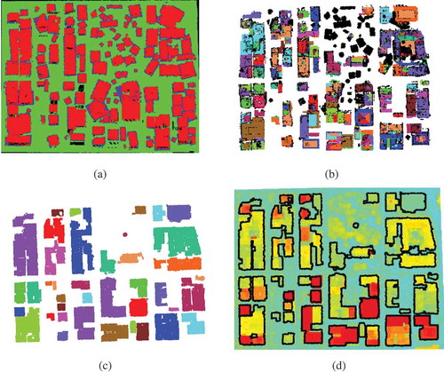
The refinement operator eliminates many false building objects and building points. Nevertheless, it may segment one building with a complex shape into several parts (Figure 2b), which should be merged to extract a complete building roof outline. The proposed method first compares the intensity of points in the adjacent cuboids detected. Then, it merges detected adjacent cuboids if the intensity difference in the adjacent cuboids is less than a threshold (e.g. 20). Figure 2c shows the results of merging detected adjacent objects. Different buildings are indicated by different colours.

3.2. Building roof outline extraction

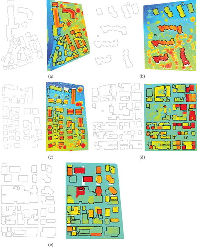
To extract the roof outlines of detected building objects, the modified convex hull method of Kwak (2013) is used. In the modified convex hull method, the size of the search window is the key factor. A too small search window cannot provide enough points, and therefore, tracing of the outline may be stopped by failure to find a subsequent point. A too large search window may contain several points of the outline, and therefore, important points of the outline may be missed. Empirically, it has been found that three times the average point spacing of the point cloud data is an appropriate size for the radius of the search window (Lahamy 2008). Using this empirical size of search window, the outlines of buildings can be extracted very well. Figure 2d shows the results of building roof outline extraction and overlap with raw point clouds.

4. Experiments and analysis

4.1. Test data-sets

The proposed model was tested with LiDAR data-sets from Vaihingen, Germany (Cramer 2010), and Toronto, Canada (five data-sets in total), in the context of the ‘ISPRS Test Project on Urban Classification and 3D Building Reconstruction’. The three areas of Vaihingen, Germany, present a typical ‘old-world’ scenario. Area 1 is characterized by dense development consisting of historic buildings with fairly complex shapes, roads and trees. Area 2 is characterized by a few high-rise residential buildings surrounded by trees. Area 3 is a purely residential area with small detached houses and many surrounding trees. The two areas of Toronto, Canada, present a typical ‘new-world’ scenario. Area 4 contains a mixture of low and high multi-story buildings, which show various degrees of shape complexity in roof structure. Area 5 presents a cluster of high-rise buildings, which is typical of North American cities. A description of the five standard data-sets is given in Table 1.

Table 1. Description of ISPRS benchmark data-sets.

Test area	Test area 1	Test area 2	Test area 3	Test area 4	Test area 5
Area range	125 × 200 m^2	170 × 190 m^2	150 × 220 m^2	530 × 600 m^2	530 × 600 m^2
Point density	3.6/m^2	4.0/m^2	3.6/m^2	6.6/m^2	6.1/m^2
Point number	70,785	111,440	106,330	1,429,369	1,312,192

4.2. Building detection results

According to the proposed method, the number, length, width, height and orientation of the cuboids should be first specified. Because the values of these parameters are not related to the final output of the Markov chain according to the principles of the marked point process, the values of these parameters are specified within a loosely defined range; for example, the length of a cuboid can range from 5 to 50 m. To avoid extreme closeness of objects, the minimum distance between objects is specified as 3.0 m. The gradient threshold for objects is set to 1.0, which means that the elevation difference between an object and its surroundings should be greater than 1.0 m. On the other hand, the parameter of the data-coherence energy term is used to distinguish objects from their surroundings and is measured by Mahalanobis distance, which is calculated as the ratio of the mean differences squared between the object’s interior and neighbouring regions and their covariances. Suppose that the inside and outside regions of a particular object have a larger Mahalanobis distance. This means that the object can be more easily distinguished from its surroundings. This is why the Mahalanobis distance was chosen to calculate the data-coherence energy term for building objects. If more false objects are detected, will be assigned a larger value to make objects and their surroundings more distinguishable, and vice versa. Second, the initial temperature has a major effect on the search for the minimum solution and its associated time costs. A high initial temperature may lead to a huge time cost; a too low initial temperature may trap the search process in a local minimum. In the present experiments, was set to 1 because the energy variation of was found to become disordered when the temperature decreased from 1000 to 1, and the energy of decreased gradually when the temperature was less than 1.0. The coefficient of decrease was set to 0.9995 to avoid a rapid decrease in temperature. The termination temperature was set to 1.0 × 10⁻⁶.

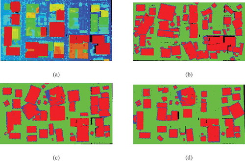
Figure 3 shows the raw ALS data and building extraction results for the five test areas. Figure 4 shows the results for building roof outlines and overlaps with the corresponding raw ALS data. The red colour and dotted blue colour in the middle figure of Figure 3 indicate the interior and the neighbourhood, respectively, of buildings. Finally, each detected building object was plotted in a single colour.

Figure 3. Benchmark data-sets and building objects detection by the proposed method (from left to right, raw point cloud, marked point process extraction results, final results after refinement). Colour figures are available in the online version of this article.

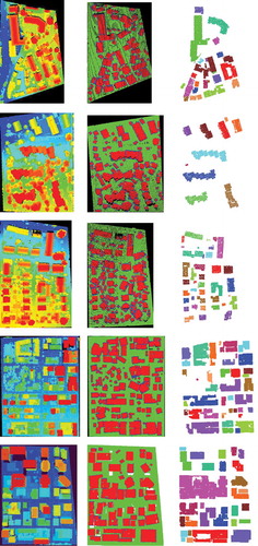
Figure 4. Building roof outlines extraction results of ISPRS benchmark data-sets by the proposed method. Colour figures are available in the online version of this article.

4.3. Evaluation and analysis

A comprehensive evaluation and comparison of building extraction performance was performed by ISPRS Workgroup III/4 based on the method described in Rutzinger, Rottensteiner, and Pfeifer (2009), which provides the completeness, correctness and quality of the results on both a per-object and a per-area level. For object-level evaluation, a building was considered to be a true positive (TP) if at least 50% of its area overlapped with the reference building. The 2D root mean square (RMS) errors of the plan metric distances of the extracted boundary points to their nearest neighbours on the corresponding reference boundaries were also provided. The per-pixel level–based evaluation results for building extraction are illustrated in Figure 5. Yellow areas represent TPs, blue areas are false negatives (FNs) and red areas are false-positive extractions (FP). Table 2 gives an evaluation of the building extraction results for the five areas. The experimental results show that the proposed method obtained very promising building extraction results. The majority of the buildings were extracted correctly (Figure 5). A few parts of buildings under ground level were missed because the proposed method assumes that buildings are higher than their surroundings. A few buildings that were surrounded by large amounts of vegetation were misclassified. In addition, a few buildings with complex shapes were not detected completely. The reason for this was that the undetected parts had a lower elevation than the main part. In test area 3, the points did not describe the complete shape of one building, also leading to incomplete detection. In test area 1, many trees were wrongly detected as buildings, resulting in a few FPs. The reason for this was that the points on the canopy exhibited a shape similar to the tops of buildings. The evaluation also shows that the RMS errors of the extracted building boundaries were less than or equal to those of the reference data-sets, demonstrating that the proposed method obtains good accuracy of building extraction.

Figure 5. Evaluation results of building extraction by the proposed method at a per-pixel level. Colour figures are available in the online version of this article.

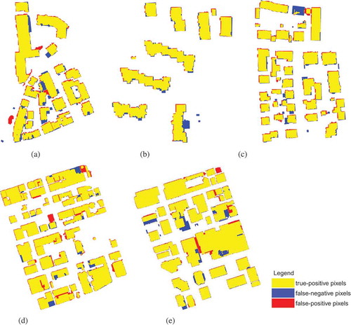
Table 2. Correctness and completeness of building extraction results by the proposed method.

Evaluation method		Area 1	Area 2	Area 3	Area 4	Area 5
Per-area	Completeness (%)	89.7	90.0	89.4	95.1	93.5
	Correctness (%)	89.6	93.9	89.1	89.3	93.2
Per-object	Completeness (%)	81.1	85.7	82.1	96.6	84.2
	Correctness (%)	96.8	100.0	95.7	94.6	97.0
Per-object >50 m^2	Completeness (%)	100.0	100.0	97.4	98.2	91.4
	Correctness (%)	96.6	100.0	97.5	94.6	97.0
RMS errors (m)		1.0	0.8	0.9	1.2	1.0

It can be seen from Table 2 that the proposed method achieves good correctness and completeness performance in extracting building objects from ALS point clouds. It extracts building objects with an average completeness of 91.5% and a correctness of 91.0% at the pixel level and with an average completeness of 85.9% (97.4%) and a correctness of 96.8% (97.1%) at the object (object >50 m²) level.

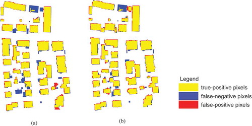
Compared with the work of Yang, Xu, and Dong (2013), the completeness of object-level building extraction was improved from 77.6 to 85.9%. The main difference from the work of Yang, Xu, and Dong (2013) is the calculation of the data-coherence energy term . The proposed method does not use the average elevation, but the lowest elevation of points in the cuboid to calculate the standard deviations of the inside and neighbouring regions of the cuboid. Simultaneously, the façade points are excluded from the calculation of the data-coherence energy term . Hence, the distinguishability of low buildings from their surroundings is significantly improved, resulting in better building detection performance, particularly in areas of buildings with small sizes and lower height. Figure 6 shows a comparison of building detection in test area 3. The completeness of the object-level evaluation increased from 73.2 to 82.1%. A full comparison between the new method (WHU_Y2) and that of Yang, Xu, and Dong (2013) (WHU_Y) and other methods can be found on the ISPRS website (ISPRS Benchmark Test 2013).

Figure 6. Comparison of building detection from test area 3 at a per-pixel level (a) building detection by Yang, Xu, and Dong (2013) and (b) building detection by the proposed method. Colour figures are available in the online version of this article.

The F1 measure was also used to compare the building extraction performance of the proposed method with that of Yang, Xu, and Dong (2013). In statistics, F1 is a measure of a test’s accuracy. The correctness and completeness of a test are both used to compute its F1 measure (Van Rijsbergen 1979). The F1 measures of the proposed method and that proposed by Yang, Xu, and Dong (2013) have been calculated and are listed in Table 3, from which it can be seen that the building extraction performance of the proposed method represents an improvement. The F1 measure can be expressed as:

(13)

Table 3. Comparison of the F1 measure of building extraction.

Name	Per-area (%)	Per-object (%)	Per-object > 50 m^2 (%)
Area 1
Yang, Xu, and Dong (2013)	89.5	88.3	98.3
The proposed method	89.6	88.3	98.3
Area 2
Yang, Xu, and Dong (2013)	91.3	88.0	100
The proposed method	91.9	92.3	100
Area 3
Yang, Xu, and Dong (2013)	87.3	83.7	94.6
The proposed method	89.2	88.4	97.4

In the light of the proposed method, the parameter is closely related to the calculation of the data-coherence energy term and has a strong effect on building extraction performance. Figure 7 provides a visual comparison of building extraction results with different values of the parameter . It shows that more false buildings were detected with a smaller value of  = 0.6 and that many buildings were omitted with a larger value of  = 1.0. The best building extraction performance was achieved with a value of  = 0.8. Hence, the value of was set to 0.8 for calculating the data-coherence energy term in this study, resulting in good extraction performance in terms of pixel-based and object-based completeness, correctness and RMS errors. However, as with all sampling-based approaches, the disadvantage of this approach is a relatively long running time. For example, the running time for the first test area was 25 minutes. The efficiency of the proposed method is related to many factors: data size, extracted object size, object discrepancies, object quantity, requirement for precision of extraction results, background complexity, parameter settings for simulated annealing and so on. Introducing graph theory or another high-efficiency optimization algorithm to improve algorithm efficiency will be a key element of future research.

Figure 7. Building extraction with different values of the data-coherence term parameter (a) raw point clouds, (b) the number of buildings = 61 (), (c) the number of buildings = 44 (), (d) the number of buildings = 42 (). Colour figures are available in the online version of this article.

5. Conclusions

This paper presents a new method based on the marked point process for extracting building objects from ALS data. Although the proposed method uses a number of algorithmic parameters, the final output is not sensitive to the majority of the parameters (e.g. the parameters of the cuboids). The experimental results showed that the proposed building detection method can achieve good performance in terms of pixel-based and object-based completeness, correctness and RMS errors. They also showed that the proposed method provides a functional and effective solution for directly extracting building objects from ALS data for a variety of scenes without resampling or gridding the input data. On the other hand, the proposed method is an object-oriented statistical geometrical method and effectively delimits the influence of noise on object detection. It is applicable for detecting buildings from ALS data with good properties. Nevertheless, the proposed method is relatively time-consuming. Improving the time performance of the proposed method for ALS data representing large scenes will be tackled in future research.

Funding

Work described in this paper is jointly supported by the National Basic Research Program of China [grant number 2012CB725301] and the National Science Foundation of China project [grant number 41071268].

Acknowledgements

The Vaihingen data-set was provided by the German Society for Photogrammetry, Remote Sensing and Geoinformation (DGPF). Special thanks go to Dr Markus Gerke at ITC, the Netherlands, for evaluating the building roof outlines extracted by the proposed method.

References

- Alharthy, A., and J. Bethel. 2002. “Heuristic Filtering and 3D Feature Extraction from LiDAR Data.” International Archives of Photogrammetry Remote Sensing and Spatial Information Sciences XXIV (part 3): 212–223.
- Bartels, M., and H. Wei. 2006. “Maximum Likelihood Classification of LIDAR Data Incorporating Multiple Co-Registered Bands.” 4th International Workshop on Pattern Recognition in Remote Sensing in Conjunction with the 18th International Conference on Pattern Recognition, Hong Kong, August 20, 17–20. Compact disc.
- Brennan, R., and T. L. Webster. 2006. “Object-Oriented Land Cover Classification of Lidar-Derived Surfaces.” Canadian Journal of Remote Sensing 32: 162–172. doi:10.5589/m06-015.
- Brenner, C. 2005. “Building Reconstruction from Images and Laser Scanning.” International Journal of Applied Earth Observation and Geoinformation 6 (3–4): 187–198. doi:10.1016/j.jag.2004.10.006.
- Cheng, L., J. Y. Gong, M. C. Li, and Y. X. Liu. 2011. “3D Building Model Reconstruction from Multi-view Aerial Imagery and LiDAR Data.” Photogrammetric Engineering & Remote Sensing 77 (2): 125–139. doi:10.14358/PERS.77.2.125.
- Cramer, M. 2010. “The DGPF-Test on Digital Airborne Camera Evaluation – Overview and Test Design.” Photogrammetrie – Fernerkundung – Geoinformation 2010 (2): 73–82. doi:10.1127/1432-8364/2010/0041.
- Green, P. 1995. “Reversible Jump Markov Chain Monte Carlo Computation and Bayesian Model Determination.” Biometrika 82 (4): 711–732. doi:10.1093/biomet/82.4.711.
- Henn, A., G. Gröger, V. Stroh, and L. Plümer. 2013. “Model Driven Reconstruction of Roofs from Sparse LIDAR Point Clouds.” ISPRS Journal of Photogrammetry and Remote Sensing 76 (2013): 17–29. doi:10.1016/j.isprsjprs.2012.11.004.
- Huang, H., C. Brenner, and M. Sester. 2013. “A Generative Statistical Approach to Automatic 3D Building Roof Reconstruction from Laser Scanning Data.” ISPRS Journal of Photogrammetry and Remote Sensing 79 (2013): 29–43. doi:10.1016/j.isprsjprs.2013.02.004.
- Im, J., J. R. Jensen, and M. E. Hodgson. 2008. “Object-Based Land Cover Classification Using High-Posting-Density LiDAR Data.” GIScience and Remote Sensing 45 (2): 209–228. doi:10.2747/1548-1603.45.2.209.
- ISPRS Benchmark Test. 2013. “Results of ‘ISPRS Test Project on Urban Classification and 3D Building Reconstruction’.” Accessed June 23, 2013. http://www2.isprs.org/commissions/comm3/wg4/results.html
- Kwak, E. 2013. “Automatic 3D Building Model Generation by Integrating LiDAR and Aerial Images Using a Hybrid Approach.” PhD thesis, University of Calgary, Canada.
- Lafarge, F., X. Descombes, J. Zerubia, and M. Pierrot-Deseilligny. 2008. “Automatic Building Extraction from DEMs Using an Object Approach and Application to the 3D-City Modeling.” ISPRS Journal of Photogrammetry and Remote Sensing 63 (3): 365–381. doi:10.1016/j.isprsjprs.2007.09.003.
- Lafarge, F., G. Gimel’farb, and X. Descombes. 2010. “Geometric Feature Extraction by a Multi-Marked Point Process.” IEEE Transactions on Pattern Analysis and Machine Intelligence 32 (9): 1597–1609. doi:10.1109/TPAMI.2009.152.
- Lafarge, F., and C. Mallet. 2012. “Creating Large-Scale City Models from 3D-Point Clouds: A Robust Approach with Hybrid Representation.” International Journal of Computer Vision 99 (1): 69–85. doi:10.1007/s11263-012-0517-8.
- Lahamy, H. 2008. “Outlining Buildings Using Airborne Laser Scanner Data.” MSc thesis, International Institute for Geo-Information Science and Earth Observation (ITC), the Netherlands.
- Lee, S. J., J. R. Kim, and Y. S. Choi. 2013. “The Extraction of Forest CO2 Storage Capacity Using High-Resolution Airborne Lidar Data.” GIScience & Remote Sensing 50 (2): 154–171.
- Lodha, S. K., D. M. Fitzpatrick, and D. P. Helmbold. 2007. “Aerial LiDAR Data Classification Using Adaboost.” International Conference on 3D Digital Imaging and Modeling, August 21–23, Montreal, QC, 435–442. IEEE.
- Lu, Y. H., J. C. Trinder, and K. Kubik. 2006. “Automatic Building Detection Using the Dempster-Shafer Algorithm.” Photogrammetric Engineering and Remote Sensing 72 (4): 395–403. doi:10.14358/PERS.72.4.395.
- Lu, Z., J. Im, and L. J. Quackenbush. 2011. “A Volumetric Approach to Population Estimation Using LiDAR Remote Sensing.” Photogrammetric Engineering & Remote Sensing 77 (11): 1145–1156. doi:10.14358/PERS.77.11.1145.
- Meng, X., L. Wang, and N. Currit. 2009. “Morphology-Based Building Detection from Airborne LIDAR Data.” Photogrammetric Engineering & Remote Sensing 75 (4): 437–442. doi:10.14358/PERS.75.4.437.
- Miliaresis, G., and N. Kokkas. 2007. “Segmentation and Object-Based Classification for the Extraction of the Building Class from LIDAR DEMs.” Computers & Geosciences 33: 1076–1087. doi:10.1016/j.cageo.2006.11.012.
- Moussa, A., and El-Sheimy. 2012. “A New Object Based Method for Automated Extraction of Urban Objects from Airborne Sensors Data.” International Archives of the Photogrammetry, Remote Sensing and Spatial Information Sciences, XXII ISPRS Congress, Vol. XXXIX-B3, Melbourne, August 25– September 1.
- Niemeyer, J., F. Rottensteiner, and U. Soergel. 2013. “Classification of Urban LiDAR Data Using Conditional Random Field and Random Forests.” Proceedings of the JURSE 2013, São Paulo, Brazil, April 21–23.
- Niemeyer, J., J. D. Wegner, C. Mallet, F. Rottensteiner, and U. Soergel. 2011. “Conditional Random Fields for Urban Scene Classification with Full Waveform LiDAR Data.” In PIA 2011, LNCS 6952, edited by U. Stilla, F. Rottensteiner, H. Mayer, B. Jutzi, and M. Butenuth, 233–244. Berlin: Springer.
- Ortner, M., X. Descombes, and J. Zerubia. 2007. “Building Outline Extraction from Digital Elevation Models Using Marked Point Processes.” International Journal of Computer Vision 72 (2): 107–132. doi:10.1007/s11263-005-5033-7.
- Perrin, G., X. Descombes, and J. Zerubia. 2005a. Point Processes in Forestry: An Application to Tree Crown Detection. Research Report, vol. 5544. Paris: INRIA.
- Perrin, G., X. Descombes, and J. Zerubia. 2005b. “A Marked Point Process Model for Tree Crown Extraction in Plantations.” IEEE International Conference on Image Processing, Genoa, September 11–14, 661–664. IEEE.
- Poullis, C., and S. You. 2009. “Automatic Reconstruction of Cities from Remote Sensor Data.” IEEE Computer Society Conference on Computer Vision and Pattern Recognition (CVPR 2009), Miami, FL, June 20–25, 2775–2782. IEEE.
- Rottensteiner, F., and C. Briese. 2002. “A New Method for Building Extraction in Urban Areas from High-Resolution LiDAR Data.” International Archives of Photogrammetry Remote Sensing and Spatial Information Sciences XXIV (part 3): 295–301.
- Rottensteiner, F., J. Trinder, S. Clode, K. Kubik, and B. Lovell. 2004. “Building Detection by Dempster-Shafer Fusion of LIDAR Data and Multispectral Aerial Imagery.” Proceedings of the 17th International Conference on Pattern Recognition, ICPR’04, Cambridge, August 23–26, 339–342. IEEE.
- Rutzinger, M., F. Rottensteiner, and N. Pfeifer. 2009. “A Comparison of Evaluation Techniques for Building Extraction from Airborne Laser Scanning.” IEEE Journal of Selected Topics in Applied Earth Observations and Remote Sensing 2 (1): 11–20. doi:10.1109/JSTARS.2009.2012488.
- Sohn, G., and I. Dowman. 2007. “Data Fusion of High-resolution Satellite Imagery and LiDAR Data for Automatic Building Extraction.” ISPRS Journal of Photogrammetry and Remote Sensing 62 (1): 43–63. doi:10.1016/j.isprsjprs.2007.01.001.
- Stoica, R., X. Descombes, and J. Zerubia. 2004. “A Gibbs Point Process for Road Extraction from Remotely Sensed Images.” International Journal of Computer Vision 57 (2): 121–136. doi:10.1023/B:VISI.0000013086.45688.5d.
- Tournaire, O., M. Brédif, D. Boldo, and M. Durupt. 2010. “An Efficient Stochastic Approach for Building Footprint Extraction from Digital Elevation Models.” ISPRS Journal of Photogrammetry and Remote Sensing 65 (4): 317–327. doi:10.1016/j.isprsjprs.2010.02.002.
- Tournaire, O., and N. Paparoditis. 2009. “A Geometric Stochastic Approach Based on Marked Point Processes for Road Mark Detection from High Resolution Aerial Images.” ISPRS Journal of Photogrammetry and Remote Sensing 64 (6): 621–631. doi:10.1016/j.isprsjprs.2009.05.005.
- Van Rijsbergen, C. J. 1979. Information Retrieval. 2nd ed. London: Butterworths.
- Vosselman, G., and S. Dijkman. 2001. “3D Building Model Reconstruction from Point Clouds and Ground Plan.” International Archives and Remote Sensing XXXIV-3/W4: 37–43.
- Yang, B. S., Z. Wei, Q. Q. Li, and J. Li. 2012. “Automated Extraction of Street-Scene Objects from Mobile Lidar Point Clouds.” International Journal of Remote Sensing 33 (18): 5839–5861. doi:10.1080/01431161.2012.674229.
- Yang, B. S., Z. Wei, Q. Q. Li, and J. Li. 2013. “Semiautomated Building Facade Footprint Extraction from Mobile LiDAR Point Clouds.” IEEE Geoscience and Remote Sensing Letters 10 (4): 766–770. doi:10.1109/LGRS.2012.2222342.
- Yang, B. S., W. X. Xu, and Z. Dong. 2013. “Automated Extraction of Building Outlines from Airborne Laser Scanning Point Clouds.” IEEE Geoscience and Remote Sensing Letters 10 (6): 1399–1403. doi:10.1109/LGRS.2013.2258887.