Effect of point density and interpolation of LiDAR-derived high-resolution DEMs on landscape scarp identification

Abstract

Recognition of geomorphic features, such as landslide scarps, is the first key step for landslide risk assessment and mitigation. Geomorphic features can be identified from high-resolution digital elevation model (DEM). Light Detection and Ranging (LiDAR) is a useful tool to collect high-density point elevation data from ground surfaces. LiDAR ground points are used to generate high-resolution DEMs. However, LiDAR sample sizes and interpolation methods are critical parameters for DEM estimation under various land cover types. To discuss the effect of the parameters, this study used a series of cases to estimate the DEMs and identify the landslide scarps, especially potential landslide scarps hidden in the forest.

Results show that LiDAR sample size affects the visual identification rate of the landslide scarps. The point density of LiDAR data controls the level of detail that can be resolved in the LiDAR-derived DEM. Given low-density LiDAR ground points, the DEM accuracy is the worst, especially in dense forest. Particularly in sparse samples, the identification rate of the landslide scarp is sensitive to the interpolation method. In sparse samples, landslide scarp identification based on Kriging-estimated DEM showed the best results among the three interpolation methods. Hence, this study provides information for the assessment of the effects of sample sizes under land cover for further geomorphic monitoring, assessment and management.

Keywords:

• LiDAR
• high-resolution DEM
• geomorphic feature identification
• landslide scarp
• point density
• interpolation

1. Introduction

Airborne laser scanning or Light Detection and Ranging (LiDAR) data are increasingly applied to identify tectonic–geomorphic features hidden by vegetation (Glenn et al. 2006; Grebby et al. 2012; Trevisani, Cavalli, and Marchi 2012; Zandbergen 2010). Regional high-resolution digital elevation models (DEMs) can be generated from airborne LiDAR data (Glenn et al. 2006). Traditional aerial photography hardly detects large-scale geomorphic features hidden under forest canopies (Lin et al. 2013b). The penetration capabilities of LiDAR facilitate the identification of geomorphic features hidden under forests in mountainous areas. LiDAR offers an opportunity to capture ground elevation data in the forest and has potential for geomorphic feature identification based on high-density LiDAR data. High-resolution DEM data can be used to derive geomorphic and hydrological parameters such as basin relief and flow path (Xie, Pearlstine, and Gawlik 2012). Previous studies showed that geomorphic features such as channel networks, debris flow channel, debris flow deposits, erosion scars and landslide scarps can be extracted using high-resolution DEM (Lin et al. 2013a, 2013b; Tarolli, Sofia, and Dalla Fontana 2012). In areas covered by vegetation, the geomorphic features related to deep-seated landslides such as their crowns and scarps could be recognized from high-resolution DEMs (Lin et al. 2013a). Lin et al. (2013b) demonstrated that geomorphic features such as fault scarps hidden under vegetation can be extracted from high-resolution DEM from an airborne LiDAR survey. High-resolution DEM aided by visualization (e.g. hillshade) provided reliable information for detailed geomorphological mapping. They found that 2-m resolution DEMs failed to detect small geomorphic features (Lin et al. 2013b). Thus, a 1-m resolution DEM is generated from a highly dense LiDAR survey in the current study to identify detailed geomorphic features (Petroselli 2012). Through the shaded relief map from high-resolution DEMs, recognition of landslide is a first key step in general for landslide monitoring and risk mitigation (Lin et al. 2013a). Clarifying the components of landslide hidden in the forest can provide information on the land cover change and land movement during and after typhoons and earthquakes (Lin et al. 2013a).

Sampling density considerably influences the accuracy of LiDAR-derived high-resolution DEMs (Heritage et al. 2009; Milan and Heritage 2012; Chu et al. 2014). Heritage et al. (2009) identified the effects of survey strategies from terrestrial laser scanning (TLS) data on geomorphological investigations of a gravel bar. They concluded that the use of a sufficient set of samples results in the correct representation of the terrain. Generally, the more LiDAR points collected, the better resolved ground surface is. However, airborne LiDAR sampling density is usually limited by flying altitude and laser shot frequency, which are budget-related factors. To discuss the effect of sampling density on DEM accuracy under land cover, a series of high-resolution DEMs were generated based on various sizes of LiDAR samples. Using various interpolation methods in sparse LiDAR samples, estimated DEM quality affected geomorphic feature identification. Past studies applied a triangulated irregular network (TIN) and various interpolation methods for DEM generation (Chaplot et al. 2006; Guo et al. 2010). In the current study, we considered three commonly used interpolation methods, namely inverse distance weighting (IDW), Kriging and TIN, with linear interpolation to generate high-resolution DEMs for landslide scarp identification under various land cover types. Landslide scarp features were identified from the shaded relief maps from the DEMs, and then, the landslide scarp length was then determined based on DEMs with respect to various sample sizes.

This study applied LiDAR-derived DEM information for landslide scarp identification in mountainous areas. A progressive procedure was conducted to demonstrate the influence of sample size and interpolation methods in landslide scarp feature identification under various land cover types. A field validation was used to assess the interpolated DEM errors when compared to reference points under various land cover types. Finally, the effects of sample size and interpolation on landslide scarp identification were determined primarily based on shaded relief maps.

2. Study area and material

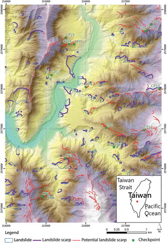
The study area covers 22 km² in the watershed (Figure 1) that is located upstream of the Tseng-Wen river in southern Taiwan. The average elevation and slope in the study area are approximately 520 m and 32°. In the study area, the land cover types are categorized as bare (bare ground), road, forest, dense forest, vegetation and low vegetation. Forest mainly comprises broadleaved trees and dense forest contains high-density ones over 1000 trees/ha. The major species of broadleaved forests include Chinese Banyan (Ficus Retusa Linn), large-leaved Nanmu (Machilus kusanoi Hayata), red cedar (Bischofia javanica Blume), Common Free Ferm (Cyathea lepifera Copel) and Chinese guger-tree (Schima superba Gardn). Areca, tea tree and bamboo are classified into vegetation; grass and crop are classified into low vegetation. In the geomorphic highlighted area (blue-green square in Figure 1), the average elevation and slope are approximately 644 m and 39°, respectively.

Figure 1. Topography and location of the study area including landslides, landslide scarps, potential landslide scarps hidden in the forest and landslide scarp checkpoints (blue-green square: highlighted area).

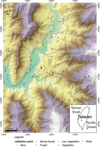
LiDAR measurements were performed in the summer, on the 23 and 24 July 2013. Global positioning system (GPS) and orientation with IMU (inertial measurement unit) were used to position the acquired LiDAR data. The airborne LiDAR data were acquired using an Optech ALTM Pegasus system (Optech Incorporated, Ontario, Canada) at 1800 m above the mean sea level. The sensors used in the systems emitted laser pulses at a wavelength of 1064 nm and a frequency of 100 KHz. The overlapped point density in the study area was approximately 37 points/m² on average, whereas the strip side overlap was more than 50%. The 269 reference points in whole study area were used based on the ground survey (Figure 2). In the study, the accuracy of LiDAR data is about 10 cm root mean square error (RMSE) vertically and 40 cm RMSE horizontally.

Figure 2. Location of 269 reference points (DEM accuracy validation points) under six land cover types, that is, bare, road, forest, dense forest, vegetation and low vegetation.

3. Method

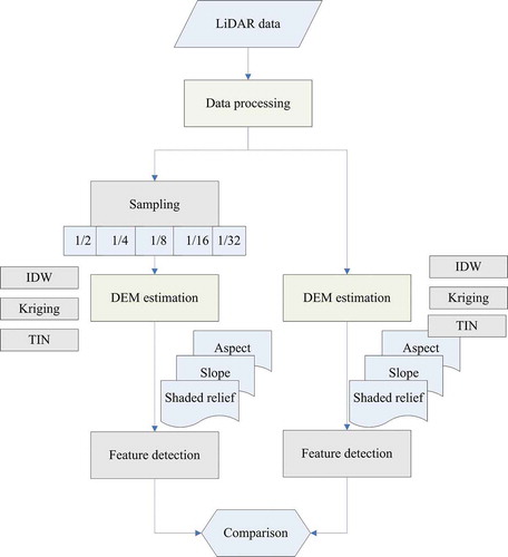
Figure 3 shows the flowchart of landslide scarp identification in the whole study area based on LiDAR-derived DEMs. The main processes in this study included data processing, sampling, DEM estimation, feature detection (landslide scarp identification) and comparison of identification results.

Figure 3. Flowchart of the landslide scarp identification based on LiDAR-derived DEMs including data processing, sampling, DEM estimation, feature detection and result comparison.

3.1. Data processing

Ground elevation was determined by the point clouds processing using TerraScan. First, non-ground points were removed out automatically. Manual editing and inspection were subsequently applied to ensure the points laying at the expected ground surface.

3.2. Sampling (LiDAR data reduction)

To evaluate the effect of point density of LiDAR data on the geomorphic feature identification, we resampled the original high-density LiDAR data with five different sizes of the original data. LiDAR samples were reacquired based on uniform sampling from laser pulse sequences. For example, a case with 1/2 samples, one is selected per two laser pulses. In this study, five sample sizes, which included 1/2, 1/4, 1/8, 1/16 and 1/32 samples, were applied. The overlapped point (total shot) densities for 1/2, 1/4, 1/8, 1/16 and 1/32 samples were equal to 18.8, 9.4, 4.7, 2.3 and 1.2 points/m², respectively. The corresponding average densities of ground points for 1/2, 1/4, 1/8, 1/16 and 1/32 samples are equal to 1.7, 0.9, 0.4, 0.2 and 0.1 points/m².

3.3. DEM estimation

High-resolution DEM can be used to detect geomorphic features without a major loss of accuracy with respect to finer resolutions (Cavalli et al. 2008). In the current study, 1-m resolution DEM was estimated from the LiDAR sampling data. In DEM estimation, three commonly used interpolation methods were applied to determine the elevation for any unmeasured location based on the measured values surrounding the estimated location. After DEM generation, a validation was applied to assess the interpolated LiDAR elevation error in each reference point under various land cover types. The elevations in 269 reference points were measured by GPS and Total Station (Figure 2).

The three interpolation approaches are described as follows:

3.3.1. IDW

IDW is a simple interpolation method. This approach assumes that each measured point has a local influence based on the weighted inverse distance. The weights are stronger where the points are closer to the estimated location than those farther away. The influence of known points on the interpolated values based on their distance from the estimated point can be controlled by defining the power. The general equation for IDW is

(1)

where is the estimated elevation value at location , is the elevation value at known location , is the distance between and for the specified power k, and s is the sample number (Equation (1); Shepard 1968). In our study, we used a power of 0.5 for interpolation.

3.3.2. Kriging

Kriging is a method that uses variogram to express the spatial variation of variables. Ordinary Kriging, which is the most widely used among the Kriging methods, is applied in this study. The longitude, latitude and elevation of LiDAR point data are Kriging inputs. Ordinary Kriging minimizes the error variance with an unbiased constraint and assigns weights according to a data-driven function (i.e. variogram model). A relatively consistent set of best-fit models with maximum r² values was generated using the least square model fitting method to fit the variogram models. An experimental variogram for the interval lag distance class h, γ(h), can be represented as

(2)

where h denotes the lag distance that separates pairs of points. Z(x_i + h) and Z(x_i) denote the elevation values at location x_i + h and location x_i, respectively. n(h) denotes the number of pairs with lag distance h (Equation (2); Journel and Huijbregts 1978; Chu et al. 2014). In this study, Surfer software was applied to determine experimental variograms and the Kriging interpolation.

3.3.3. TIN with linear interpolation

A TIN is arranged in a network of non-overlapping triangles. For the representation of a grid surface terrain, TINs combined with linear interpolation were used to generate rasterized elevation data. The interpolated elevation is the linear weighted sum of elevations of its surrounding triangle vertices (Heritage et al. 2009).

3.4. Feature detection (landslide scarp identification)

Geomorphic features directly appear from the three-dimensional (3D) visualization of DEMs. From the DEMs, commonly used geomorphic images, including shaded relief, slope and aspect maps, were obtained. Among these images, the shaded relief image allowed a 2.5D geomorphic expression that impressively represented the subtle topography in detail and was useful in identifying the landslide scarp hidden in the forest. Since landslide scarp is a relatively steep surface at the upper edge of the landslide, landslide scarp can be easily identified from the shaded relief map of high-resolution DEMs. After feature detection, field validations of scarp detection were checked at 15 locations of study area (green points in Figure 1).

3.5. Comparison of identification results

In this study, the feature identification was primarily based on shaded relief maps from DEMs. After feature detection in various cases, the landslide scarp length percentages (i.e. the ratio of the total scarp length in the sampled DEM versus the total scarp length in the reference DEM) were evaluated using sampling data compared with results using whole data (like-for-like comparisons, e.g. IDW-derived DEM vs. IDW-derived reference DEM). In this study, the reference DEM was interpolated using each interpolation based on whole data.

4. Results and discussion

4.1. Feature identification from high-resolution DEMs

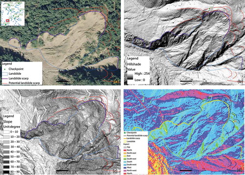
A set of terrain parameters, which include shaded relief, slope, curvature and aspect, from the high-resolution DEMs can be enhanced by the visual interpretation of geomorphologies (Trevisani, Cavalli, and Marchi 2012). Figure 4 shows a landslide example in shaded relief, slope and aspect maps. The principal data-set used in landslide mapping is the shaded relief because the most landslides contain the slide body with steepened sides occurring towards the toe. Landslide scarps are identified due to relatively steep surfaces at the upper edge of the landslides. In addition, the slope in the example contributes most whose aspect is towards south, west and south-west (Figure 4(d)). Figure 1 also shows the results from geomorphic feature identification using high-resolution DEMs that considered the whole LiDAR data-set. The purple line represents the explicit landslide area and landslide scarp, most of which are shallow landslides that can be identified easily using only multitemporal satellite or aerial images. The red line represents the potential landslide scarp hidden in forest, and some belong to deep-seated landslides. However, deep-seated landslides are difficult to detect using multitemporal images (Lin et al. 2013a). From LiDAR-derived high-resolution DEMs, the DEMs allowed the detection of detailed damage signatures, such as deep-seated landslides and their scarps (Lin et al. 2013a). High-resolution DEMs also provide the ability to characterize the local topographic surface texture and high-resolution geomorphology in large areas. For geomorphology, the DEM texture provides useful information that is strictly linked to active geomorphic processes (Chambers et al. 2011).

Figure 4. Landslides, landslide scarps and potential landslide scarps hidden in the forest in (a) photo, (b) shaded relief, (c) slope and (d) aspect maps at the checkpoint (CP3).

4.2. Effects of sample density on DEM accuracy

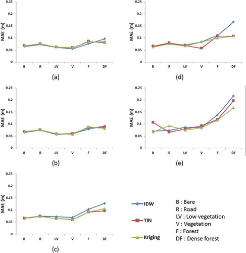
Figure 5 shows the spatial pattern of sampling density in highlighted area (blue-green square in Figure 1). Because LiDAR penetration depends on land cover types, spatial patterns of LiDAR densities are heterogeneous in various land cover types. In highlighted area, average ground point densities from various land cover types for 1/2, 1/4, 1/8, 1/16 and 1/32 samples are shown in Table 1. At the upper-right corner (yellow polygon) of Figure 5, LiDAR point clouds hardly penetrate the dense forest, and few ground point samples are found. The sampling density is higher in bare land and low vegetation than other land cover (Table 1 and Figure 5). Sampling density under various land cover types generally affects the accuracy of high-resolution DEM. Upon validation (Figure 6) based on reference points in study area, the results of the mean absolute errors (MAEs) of elevations were less than 10 cm, which are consistent in the three interpolation methods when sample sizes are greater than 1/8 samples (4.7 points/m² in total shots). In sparse samples (lower than 4.7 points/m²), the MAEs were greater than 10 cm, especially in forest and dense forest. For high-density LiDAR samples, IDW is a simple and suitable interpolator (Liu 2008). To reduce data redundancy and increase the computation efficiency, LiDAR data sampling (data reduction) is important in DEM generation (Liu 2008). For geomorphic application, data reduction will cause some problems. When sample density decreases in forest and dense forest, the DEM accuracy decreases, particularly in IDW. Given a low-density of ground point data, the DEM accuracy is the worst in the dense forest. In 1/32 samples (1.2 points/m²), the MAEs using three methods are greater than 15 cm in the dense forest. Results show that the performance in Kriging is better than in other methods in sparse samples. These results are consistent with the results from previous studies (Guo et al. 2010; Lloyd and Atkinson 2002), in which the interpolation methods used, such as IDW and TIN with linear interpolation, efficiently generated DEMs from sufficient LiDAR data; Kriging methods are the most reliable. LiDAR sample density is the key factor affecting the accuracy of high-resolution DEM. Increasing sampling density can reduce the uncertainty of interpolation. Generally, the vertical accuracy of LiDAR-derived DEM that is estimated at approximately 15 cm using ground survey points depends on various terrain, land cover types and LiDAR systems (Habib 2008; Jaboyedoff et al. 2012). In the current study, the vertical accuracy of DEM in most cases was under 15 cm. From the results, the vertical accuracy of DEM is highly dependent on sample density and interpolation methods, particularly in 1/32 samples. For increasing DEM accuracy, a critical factor is the proper selection of the sample points in sparse samples to eliminate extrapolations from the computational process (Gosciewski 2013).

Table 1. Average ground point densities from various land cover types for 1/2, 1/4, 1/8, 1/16 and 1/32 samples in geomorphic highlighted area (unit: points/m²).

	1/2 samples	1/4 samples	1/8 samples	1/16 samples	1/32 samples
Dense forest	0.86	0.43	0.22	0.11	0.06
Forest	1.35	0.67	0.33	0.17	0.08
Low vegetation	1.95	0.98	0.49	0.25	0.12
Bare	3.81	1.91	0.97	0.48	0.24

Figure 5. Spatial pattern of sample density (unit: points/m²) in geomorphic highlighted area for (a) 1/2, (b) 1/4, (c) 1/8, (d) 1/16, (e) 1/32 samples and (f) aerial photo image.

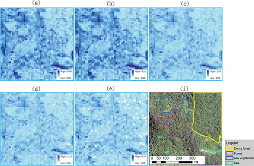
Figure 6. Mean absolute errors (MAEs) of estimated DEMs based on three interpolation methods for (a) 1/2, (b) 1/4, (c) 1/8, (d) 1/16 and (e) 1/32 samples under various land cover types (number of reference points are 42 in bare land (B), 65 in road (R), 42 in low vegetation (LV), 40 in vegetation (V), 38 in forest (F) and 42 in dense forest (DF)).

4.3. Effects of sample sizes and interpolation methods for scarp identification

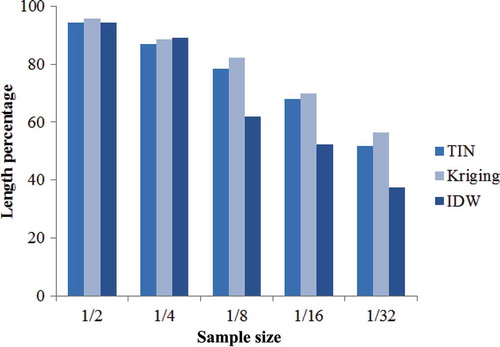
Identification results of landslide scarp were validated in 15 field locations (field photographs shown in Figure 7). Figures 8–10 show the landslide scarp identification results in the highlighted area on the basis of the DEMs with various sample sizes using the three interpolation methods. The DEMs become fuzzy when sparse sample sizes are used, particularly in IDW. In IDW, the DEMs for 1/8, 1/16 and 1/32 samples are non-smooth and rugged (Figure 8). The landslide scarp identification based on the DEMs of Kriging and TIN with linear interpolation (Figures 9 and 10) is better than that of IDW (Figure 8), particularly in sparse sample sizes. In 3D model, the DEM difference (e.g. mountainous roads) can be easily detected, especially between 1/2 samples (Figure 11(a)) and 1/32 samples (Figure 11(b)) based on TIN method. The large triangular surface exists due to few sample points in Figure 11(b). In geomorphic investigations, the more common LiDAR point densities are 1 point/m² to 3 points/m², but the suitable ones are over 5 points/m² under vegetation (Milan and Heritage 2012; Chu et al. 2014). This rule is similar to the current study, in which poor-quality high-resolution DEM was obtained when the sample size was under 1/8 samples (i.e. density is about 4.7 points/m²). The sample size under 4.7 points/m² is not allowable when DEM accuracy is the major concern for geomorphic feature identification in the mountainous area. Figure 12 shows that, in terms of identification (detection) rate, Kriging outperforms other methods in the same sampling sets, particularly for few samples. Kriging provides the information on the spatial structure of data (i.e. distance and variation between sampling data), particularly in the low-density LiDAR data (Liu 2008). The identification rate for landslide scarp length decreases as the sample size decreases. Based on 1/8 samples, the identification rates for length percentages relative to whole samples were 82.2%, 78.4% and 61.8% for Kriging, TIN with linear interpolation and IDW, respectively. The performances of feature detection on the basis of various DEMs for Kriging and TIN with linear interpolation are better than those of IDW, particularly in sparse sample sizes. In sparse samples (lower than 4.7 points/m²), geomorphic feature identification is sensitive to interpolation methods. Based on IDW, the estimated DEM becomes fuzzy, and the scarp feature is difficult to recognize in sparse samples. The results also show that feature identification rates using Kriging are larger than 80% when the LiDAR data are over 1/8 samples (4.7 points/m²). From the case studies, LiDAR density over 4.7 points/m² is required in the identification of landslide scarps.

This study reveals the potential of geomorphic applications from LiDAR data when high-resolution DEM becomes available. From a practical standpoint, it would be useful to combine LiDAR and multispectral images for further geomorphic applications.

Figure 7. Field photographs of landslide scarps and potential landslide scarps hidden by vegetation in the checkpoints ((a) CP1, (b) CP7, (c) CP10, (d) CP3, (e) CP5, (f) CP6) referring to Figure 1.

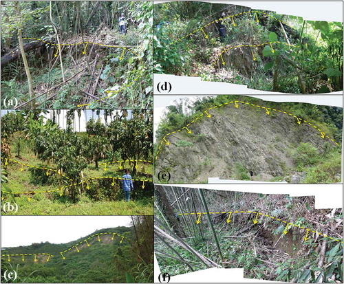
Figure 8. Landslide scarp identification from IDW-derived DEMs based on (a) whole data, (b) 1/2, (c) 1/4, (d) 1/8, (e) 1/16 and (f) 1/32 samples in geomorphic highlighted area.

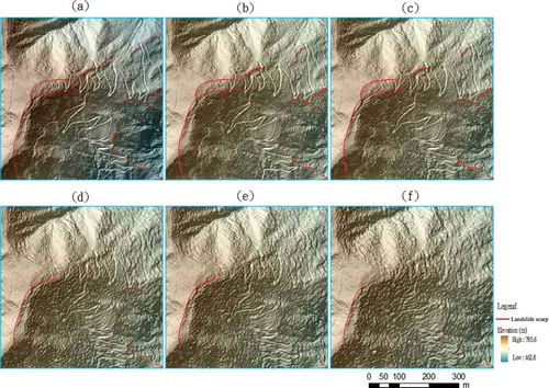
Figure 9. Landslide scarp identification from Kriging-derived DEMs based on (a) whole data, (b) 1/2, (c) 1/4, (d) 1/8, (e) 1/16 and (f) 1/32 samples in geomorphic highlighted area.

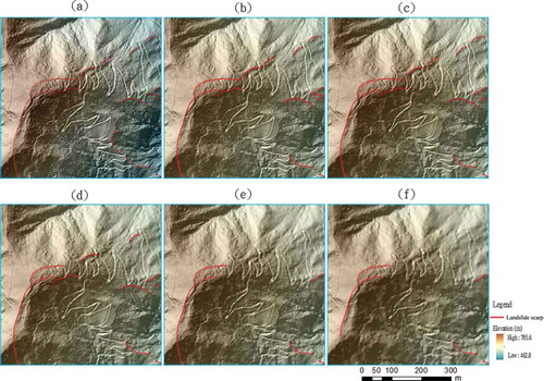
Figure 10. Landslide scarp identification from TIN-derived DEMs based on (a) whole data, (b) 1/2, (c) 1/4, (d) 1/8, (e) 1/16 and (f) 1/32 samples in geomorphic highlighted area.

Figure 11. 3D model of TIN based on (a) 1/2 samples and (b) 1/32 samples.

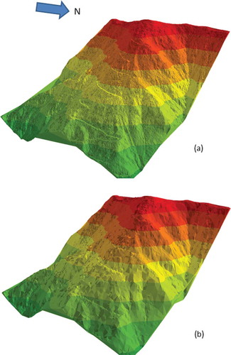
Figure 12. Length percentage of landslide scarp identification (i.e. the ratio of the total scarp length in the sampled DEM to the total scarp length in the reference DEM) based on various sizes of samples and three interpolation methods, that is, IDW, Kriging and TIN with linear interpolation.

5. Conclusion

This study quantified the effects of sample sizes and interpolation methods on geomorphic feature identification in a mountainous area. Results showed that LiDAR offers a reasonably efficient approach to ensure excellent identification of geomorphic features hidden under vegetation. Sample size substantially influences high-resolution DEM estimation, and the DEM quality affects landslide scarp identification. Generally, an increase in sampling density can reduce the DEM uncertainty. The penetration of LiDAR usually depends on land cover types. DEM uncertainty is highly dependent on the land cover types in sparse LiDAR samples. In a dense forest, penetrating LiDAR points are few, reducing the DEM accuracy. Landslide scarp identification is also primarily based on the details of shaded relief maps from DEMs. The LiDAR-derived DEMs in the recognition of geomorphological features provided the feasibility of distinguishing landslide scarps in the study area. Based on sampling data, the landslide scarp length percentages were evaluation indices compared with results using whole data-set. In sparse LiDAR samples, landslide scarp identification is sensitive to interpolation methods in the dense forest. The performances of feature detection on the basis of various DEMs for Kriging and TIN with linear interpolation are better than those of IDW, particularly in sparse sample sizes. Kriging- and TIN-estimated high-resolution DEMs display the excellent performance in visual identification of landslide scarp. The proposed model, which underwent a series of tests, can provide information that can effectively facilitate the identification of geomorphic features from high-resolution DEMs. Further study will develop the automatic scheme for landslide scarp identification.

Funding

This work was supported by Department of Land Administration, Ministry of Interior of Taiwan, R.O.C. [grant number SYC1020117].

Conflict of Interest

The authors declare no conflict of interest.

Acknowledgements

The authors thank the editors and reviewers for their valuable comments and suggestions and Dr JoChi Lin for the data processing discussion.

References

- Cavalli, M., P. Tarolli, L. Marchi, and G. Dalla Fontana. 2008. “The Effectiveness of Airborne LiDAR Data in the Recognition of Channel Bed Morphology.” Catena 73: 249–260. doi:10.1016/j.catena.2007.11.001.
- Chambers, J. E., P. B. Wilkinson, O. Kuras, J. R. Ford, D. A. Gunn, P. I. Meldrum, C. V. L. Pennington, A. L. Weller, P. R. N. Hobbs, and R. D. Ogilvy. 2011. “Three-Dimensional Geophysical Anatomy of an Active Landslide in Lias Group Mudrocks, Cleveland Basin, UK.” Geomorphology 125 (4): 472–484. doi:10.1016/j.geomorph.2010.09.017.
- Chaplot, V., F. Darboux, H. Bourennane, S. Leguédois, N. Silvera, and K. Phachomphon. 2006. “Accuracy of Interpolation Techniques for the Derivation of Digital Elevation Models in Relation to Landform Types and Data Density.” Geomorphology 77 (1–2): 126–141. doi:10.1016/j.geomorph.2005.12.010.
- Chu, H.-J., R.-A. Chen, Y.-H. Tseng, and C.-K. Wang. 2014. “Identifying LiDAR Sample Uncertainty on Terrain Features from DEM Simulation.” Geomorphology 204: 325–333. doi:10.1016/j.geomorph.2013.08.016.
- Glenn, N. F., D. R. Streutker, D. J. Chadwick, G. D. Thackray, and S. J. Dorsch. 2006. “Analysis of LiDAR-Derived Topographic Information for Characterizing and Differentiating Landslide Morphology and Activity.” Geomorphology 73 (1–2): 131–148. doi:10.1016/j.geomorph.2005.07.006.
- Gosciewski, D. 2013. “Selection of Interpolation Parameters Depending on the Location of Measurement Points.” GIScience & Remote Sensing 50 (5): 515–526.
- Grebby, S., D. Cunningham, J. Naden, and K. Tansey. 2012. “Application of Airborne LiDAR Data and Airborne Multispectral Imagery to Structural Mapping of the Upper Section of the Troodos Ophiolite, Cyprus.” International Journal of Earth Sciences 101 (6): 1645–1660. doi:10.1007/s00531-011-0742-3.
- Guo, Q., W. Li, H. Yu, and O. Alvarez. 2010. “Effects of Topographic Variability and LiDAR Sampling Density on Several DEM Interpolation Methods.” Photogrammetric Engineering and Remote Sensing 76 (6): 701–712. doi:10.14358/PERS.76.6.701.
- Habib, A. 2008. “Accuracy, Quality Assurance and Quality Control of LiDAR Data, Chap 9.” In Topographic Laser Ranging and Scanning: Principles and Processing, edited by J. Shan and C. K. Toth, 269–294. Boca Raton, FL: CRC Press, Taylor & Francis.
- Heritage, G. L., D. J. Milan, A. R. G. Large, and I. C. Fuller. 2009. “Influence of Survey Strategy and Interpolation Model on DEM Quality.” Geomorphology 112: 334–344. doi:10.1016/j.geomorph.2009.06.024.
- Jaboyedoff, M., T. Oppikofer, A. Abellán, M.-H. Derron, A. Loye, R. Metzger, and A. Pedrazzini. 2012. “Use of LiDAR in Landslide Investigations: A Review.” Natural Hazards 61 (1): 5–28. doi:10.1007/s11069-010-9634-2.
- Journel, A. G., and C. H. J. Huijbregts. 1978. Mining Geostatistics. London: Academic Press.
- Lin, C.-W., C.-M. Tseng, Y.-H. Tseng, L.-Y. Fei, Y.-C. Hsieh, and P. Tarolli. 2013a. “Recognition of Large Scale Deep-Seated Landslides in Forest Areas of Taiwan Using High Resolution Topography.” Journal of Asian Earth Sciences 62: 389–400. doi:10.1016/j.jseaes.2012.10.022.
- Lin, Z., H. Kaneda, S. Mukoyama, N. Asada, and T. Chiba. 2013b. “Detection of Subtle Tectonic Geomorphic Features in Densely Forested Mountains by Very High-Resolution Airborne LiDAR Survey.” Geomorphology 182: 104–115. doi:10.1016/j.geomorph.2012.11.001.
- Liu, X. 2008. “Airborne LiDAR for DEM Generation: Some Critical Issues.” Progress in Physical Geography 32 (1): 31–49. doi:10.1177/0309133308089496.
- Lloyd, C. D., and P. M. Atkinson. 2002. “Deriving DSM from LiDAR Data with Kriging.” International Journal of Remote Sensing 23 (12): 2519–2524. doi:10.1080/01431160110097998.
- Milan, D. J., and G. L. Heritage. 2012. “LiDAR and ADCP Use in Gravel Bed Rivers: Advances since GBR6.” In Gravel-bed Rivers: Processes, Tools, Environments, edited by M. Church, P. Biron, and A. Roy, 286–302. Chichester: John Wiley & Sons.
- Petroselli, A. 2012. “LiDAR Data and Hydrological Applications at the Basin Scale.” GIScience & Remote Sensing 49 (1): 139–162. doi:10.2747/1548-1603.49.1.139.
- Shepard, D. 1968. “A Two-dimensional Interpolation Function for Irregularly-spaced Data.” Proceedings of the 1968 ACM National Conference, 517–524. doi:10.1145/800186.810616.
- Tarolli, P., G. Sofia, and G. Dalla Fontana. 2012. “Geomorphic Features Extraction from High-Resolution Topography: Landslide Crowns and Bank Erosion.” Natural Hazards 61: 65–83. doi:10.1007/s11069-010-9695-2.
- Trevisani, S., M. Cavalli, and L. Marchi. 2012. “Surface Texture Analysis of a High-Resolution DTM: Interpreting an Alpine Basin.” Geomorphology 161–162: 26–39. doi:10.1016/j.geomorph.2012.03.031.
- Xie, Z., L. Pearlstine, and D. E. Gawlik. 2012. “Developing a Fine Resolution Digital Elevation Model to Support Hydrological Modeling and Ecological Studies in the Northern Everglades.” GIScience and Remote Sensing 49: 664–686. doi:10.2747/1548-1603.49.5.664.
- Zandbergen, P. A. 2010. “Accuracy Considerations in the Analysis of Depressions in Medium-Resolution LiDAR Dems.” GIScience & Remote Sensing 47 (2): 187–207. doi:10.2747/1548-1603.47.2.187.