Expansion of LISS III swath using AWiFS wider swath data and contourlet coefficients learning

Abstract

Spaceborne sensors have limited capability to acquire images with wider swath at high spatial and high temporal resolutions simultaneously. This study reports a ground processing technique that combines images from two sensors onboard Resourcesat-2 (RS2) Linear Imaging and Self-Scanning Sensor (LISS III) and an Advanced Wide-Field Sensor (AWiFS) to overcome this limitation. The spatial resolution of LISS III is 23.5 × 23.5m and that of AWiFS is 56 × 56m. The temporal resolution of LISS III is 24 days and that of AWiFS is 5 days. The 140-km swath of the LISS III overlaps at center portion of 740-km swath of AWiFS in simultaneous acquisition. Assume that the nonoverlapping region of the AWiFS contains similar Earth’s surface features of the LISS III overlapping region; then, it is possible to enhance the spatial resolution of AWiFS to the spatial resolution of LISS III in the nonoverlapping region. With this assumption, we propose a novel technique to enhance the spatial resolution of the nonoverlapping region through a single-image super-resolution technique using nonsubsampled contourlet transform (NSCT) and evaluated it on RS2 data-sets. The proposed method can create a synthetic image with 740-km swath at 23.5 × 23.5m spatial and 5-day temporal resolutions. Experimental results demonstrated that it outperforms the support vector regression (SVR)-based methods in prediction accuracy and computational time.

Keywords:

• single-image super-resolution
• swath expansion
• nonsubsampled contourlet transform (NSCT)
• AWiFS and LISS III sensors data

1. Introduction

In precision agriculture, identifying the spatial and temporal variability of crops in larger study areas is vital for the generalized decision support systems that are defined for an agricultural land use (Auernhammer 2001). Floods may affect the agricultural lands in monsoon (Sanyal and Lu 2004). Flood forecasting and natural hazard monitoring require wider swath data as, for example, data of the entire watersheds with high temporal repetition and high spatial resolution (Loew, Ludwig, and Mauser 2006). Watershed is a basic ecosystem. An ecosystem function over larger areas (entire ecosystems) is an invaluable integrated measurement of the environment and land cover (Kerr and Ostrovsky 2003). Land cover classification of high spatial data is useful for straightforward identification of vegetation types and derivation of habitats (Gillespie et al. 2008). Temporal analysis can be extrapolated to predict future ecological and land-cover changes, for instance, to estimate the result of anthropogenic land-use practices on protected species (Kerr and Ostrovsky 2003). All these remote sensing applications such as precision agriculture, flood forecasting, natural hazard monitoring, entire ecosystems and land-cover changes require images with wider swath at high spatial and temporal resolutions.

But global satellite remote sensing systems have technological limitations to acquire an image with wider swath at high spatial and temporal resolutions simultaneously. Swath width is directly proportional to the ground sampling distance (GSD) and inversely proportional to the revisit time (Coops et al. 2006). Another possible way to get images with larger swath at high spatial and high temporal resolutions is to enhance the coarser spatial resolution of an image to the fine spatial resolution at ground data processing system. Coarser spatial resolution of an image can be enhanced through single-image super-resolution techniques (Jiji and Chaudhuri 2006).

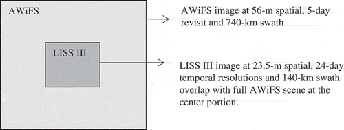
The Resourcesat-2 that is one of the Indian Space Research Organization (ISRO) mission carries the Linear Imaging and Self-Scanning Sensor (LISS III) and an Advanced Wide-Field Sensor (AWiFS). The spatial resolution of LISS III is and that of AWiFS is . The temporal resolution of LISS III is 24 days and that of AWiFS is 5 days. Table 1 describes the Resourcesat-2 AWiFS and LISS III sensors’ characteristics (ISRO 2012). The 140-km swath of LISS III overlaps with the 740-km swath of AWiFS at center portion in simultaneous acquisition as shown in Figure 1. The 140-km swath of LISS III can be expanded to the 740-km swath if the nonoverlapping region of AWiFS contains similar Earth’s surface features of LISS III overlapping region. The overlapped LISS III image and its corresponding AWiFS image were used as a prior knowledge to enhance the spatial resolution of nonoverlapping region by using a single-image super-resolution technique.

Table 1. Resourcesat-2 AWiFS and LISS III sensors’ characteristics.

	AWiFS	LISS III
Spatial resolution	56 m	23.5 m
Swath width	740 km	140 km
Spectral bands ()	B2: 0.52–0.59	B2: 0.52–0.59
	B3: 0.62–0.68	B3: 0.62–0.68
	B4: 0.77–0.86	B4: 0.77–0.86
	B5: 1.55–1.70	B5:1.55–1.70
Temporal resolution	(Revisit) 5 days	24 days

Figure 1. Overlapped LISS III at the center portion of full AWiFS scene in simultaneous acquisition.

Single-image super-resolution (Baker and Kanade 2002; Freeman, Jones, and Pasztor 2002; Chang, Yeung, and Xiong 2004; Elad and Datsenko 2009) was first proposed by Baker and Kanade (2002). They attempts to capture prior correspondence between low-resolution (LR) and high-resolution (HR) image patches and apply this correspondence to predict an HR image from an LR image. Single-image super-resolution is formulated as a kernel learning problem and predicted the high frequency details using a support vector regression (SVR) (Kim, Kim, and Kim 2004; Ni and Nguyen 2007; Srivastava et al. 2013; Islam et al. 2014).

Zhang and Huang (2013) recently proposed a single-image super-resolution through an SVR for the remote sensing images. Support vector machines (SVM) typically used for pattern recognition problems with small number of training samples (Kim et al. 2014; Güneralp, Filippi, and Hales 2013; La Rosa and Wiesmann 2013; Li, Im, and Beier 2013; Ishak et al. 2013). An SVM was later applied to the regression estimation, known as SVR (Drucker et al. 1997). An SVR takes a vector-valued input and gives a scalar-valued output. In SVR, for each pixel, we have to train an SVR model with a set of relevant HR pixel–LR patch pairs. The trained model predicts an HR pixel corresponding to the given LR patch. Although SVR has good prediction accuracy with minimum number of trained data samples, it cannot preserve the neighborhood relationship with surrounding pixels because its prediction process is pixelwise. If we predict patchwise with one or two pixels overlap, we can preserve the neighborhood relationship with the surrounding pixels. Consequently, the computational time also reduced.

2. Background

Single-image super-resolution creates an HR image from an LR image by using a set of relevant LR–HR local patches as prior. This prior knowledge is obtained from a numerous LR–HR image pairs (Kim and Kwon 2010). These image pairs would not contain the input LR image and its corresponding HR image. Our swath expansion through spatial resolution enhancement is considered as a single-image super-resolution problem. A single-image super-resolution requires a prior knowledge about the desired HR image. A prior knowledge regularizes the predicted HR image in single-image super-resolution (Milanfar 2010). But in our swath expansion problem, prior knowledge is limited to the overlapped LISS III image and its corresponding AWiFS image. Assume that the nonoverlapping region of AWiFS contains similar Earth’s surface features of overlapped LISS III image. Then, it is possible to enhance the spatial resolution of AWiFS to spatial resolution of LISS III in the nonoverlapping region. With this assumption, the limited prior knowledge makes it possible to enhance the spatial resolution of the nonoverlapping region.

Single-image super-resolution methods either make use of training data of LR–HR local patches obtained from numerous LR–HR image pairs or use an appropriate smoothness constraint with the learning prior to improving the results (Milanfar 2010). But in our method, the training data of LR–HR local patches are limited to the overlapped LISS III image and its corresponding AWiFS image. Also, any smoothness constraint was not applied in our method because LR–HR local patches were extracted over the contourlet domain. The contourlet transform (CT) has the capability to capture smoothness along contours while learning the edge primitives from the training data of LR–HR local patches over the contourlet domain (Jiji, Joshi, and Chaudhuri 2004).

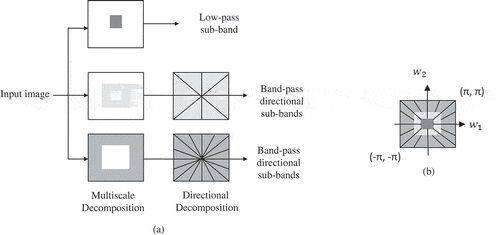
Multiresolution decomposition of an image in multiple directions gives detailed geometrical information of the content in an image (Li, Yang, and Hu 2011). This geometrical information gives high prediction accuracy in training and prediction of local patches over multiresolution domain than in spatial domain. If we predict patchwise with one or two pixels overlap, we can make it possible to preserve the neighborhood relationship with the surrounding pixels. Edges and its surrounding pixels are important to enhance the spatial resolution of an image in single-image super-resolution. The nonsubsampled contourlet transform (NSCT) preserves edges in multiresolution decomposition due to its shift invariance property (Da Cunha, Zhou, and Do 2006).

2.1. Nonsubsampled contourlet transform (NSCT)

Do and Vetterli (2005) proposed CT to represent two-dimensional singularities of an image. The CT composed of Laplacian pyramid (LP) and directional filter bank (DFB). Although CT represents curves sparsely due to its directionality and anisotropy, there is a frequency aliasing in the process of decomposition and reconstruction of an image in the CT. To reduce the frequency aliasing and enhance directional selectivity and shift invariance, Da Cunha, Zhou, and Do (2006) proposed NSCT based on nonsubsampled pyramid decomposition and nonsubsampled filter banks (NSFB). NSCT is the shift-invariant version of CT. NSCT uses iterated nonseparable two-channel NSFB to obtain the shift invariance and to avoid pseudo-Gibbs phenomena around singularities.

NSCT not only provides multiresolution analysis, but also contains geometric and directional representation. Figure 2 shows the overview of the NSCT, and Figure 2(a) shows NSFB structure. The NSCT structure is composed of filter banks which split the 2D frequency plane into sub-bands. Frequency partitioning is illustrated in Figure 2(b). NSCT gets the perfect reconstruction through reconstructing filter banks (Hu and Li 2012). NSCT is more efficient than other multiresolution analysis in image denoising and image enhancement due to its multiscale, multidirection, anisotropy and shift invariance (Da Cunha, Zhou, and Do 2006). Therefore, we perform multiresolution decomposition on remote sensing images by NSCT to enhance the spatial resolution through contourlet coefficients learning (CCL).

Figure 2. Nonsubsampled contourlet transform. (a) Nonsubsampled filter banks structure that implements the NSCT. (b) Frequency partitioning which is obtained with the filter banks shown in (a). Source: Da Cunha, Zhou, and Do (2006). © IEEE. Reproduced by permission of IEEE.

2.2. Contourlet coefficients learning (CCL)

The NSCT decomposes an image into sub-bands in multiple directions, multiple levels with shift invariance property. Each sub-band represents contourlet coefficients. These contourlet coefficients were used to build the training data between the overlapped LISS III image and its corresponding AWiFS image. These training data were used to predict the LISS III pixels with AWiFS image for the nonoverlapping region in each sub-band. This learning process of the coefficients in the contourlet transform domain is referred to as CCL.

In this article, we propose a novel technique to enhance the spatial resolution through a single-image super-resolution technique over NSCT domain. For each sub-band, training data are created in the NSCT domain. The training data contain contourlet coefficients in patchwise, and these patches have AWiFS and LISS III correspondence. This correspondence gives a desired LISS III patch through proposed CCL for a given AWiFS patch in both overlapping and nonoverlapping regions for each sub-band. The predicted sub-bands reconstruct the desired image with inverse NSCT. The reconstructed image contains the spatial resolution of LISS III in both overlapping and nonoverlapping regions of AWiFS.

3. Methodology

3.1. Training phase

To maintain AWiFS and LISS III image pixels in one-to-one correspondence, AWiFS image pixels are interpolated to the size of LISS III image pixels in geometric correction. Consequently, pixels in the overlapping region of AWiFS and LISS III images are in one-to-one correspondence. Training data for each sub-band were created by applying the NSCT to the overlapped LISS III and its corresponding interpolated AWiFS image as shown in Figure 3.

Figure 3. Training phase of the overlapping regions of AWiFS and LISS III images over NSCT domain.

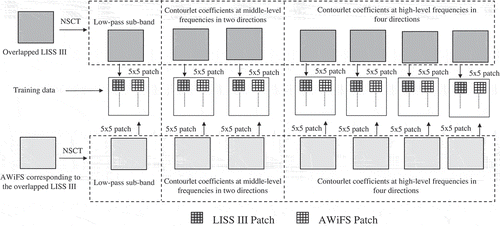
1. Extract the overlapped LISS III and its corresponding AWiFS image portion from the full AWiFS scene.

2. Apply the NSCT to the LISS III and its AWiFS image. The two-level decomposition was applied in the NSCT. Middle-level frequencies were decomposed into two directions, and high-level frequencies were decomposed into four directions. The remaining frequencies were in low-pass sub-band.

3. Extract patches with moving window, this window moves toward right side by one column. After the end of the columns, it moves down by one row. Repeat the same procedure until covering the whole sub-band. The training data were created for each sub-band in each level and direction.

Each row in training data contains pixels of LISS III patch and its corresponding pixels of AWiFS patch of the overlapping region as shown in second row of the Figure 3. These patches are rearranged into arrays to simplify the searching and identification of the desired LISS III patch corresponding to a given AWiFS patch. Training phase of the overlapped LISS III image and its corresponding AWiFS image is shown in Figure 3. Dark gray color sub-bands in the first row correspond to the overlapped LISS III image and light gray color sub-bands in the third row correspond to AWiFS image in the overlapping region. Second row represents the training data for each level and direction.

3.2. Prediction phase

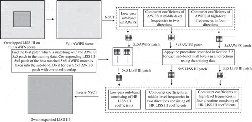
Objective of the current study was to enhance the spatial resolution of nonoverlapping region of AWiFS image to the spatial resolution of LISS III image. Interpolated full AWiFS image contains both overlapping and nonoverlapping regions. The interpolated full AWiFS image is taken as an input image to enhance the spatial resolution of the nonoverlapping region.

1. Apply NSCT to the interpolated full AWiFS scene. The number of levels and the number of directions are same as in training phase.

2. Extract a patch from a sub-band. Identify the best matched AWiFS sub-band patch in the training data where the root mean squared error (RMSE) is minimum between the given AWiFS patch and all AWiFS patches in the training data.

3. The corresponding LISS III patch of the best matched AWiFS patch is the desired LISS III patch. Move this window with one-pixel overlap and repeat the same procedure until covering the whole sub-band. An average was taken between the pixels in one-pixel overlap.

4. Apply inverse NSCT to the predicted sub-bands. The HR LISS III image is created for both the overlapping and nonoverlapping regions. Hence, the spatial resolution of nonoverlapping region is enhanced to the spatial resolution of LISS III.

In Figure 4, light gray color represents the AWiFS image pixels and dark gray color represents the LISS III image pixels. The patches were taken with one-pixel overlap to maintain the neighborhood relationship with the surrounding patches. The proposed method creates a synthetic image with wider swath at high spatial resolution. Since the revisit time of AWiFS image is 5 days, we can create a synthetic image at 740-km swath at spatial and 5-day temporal repetition.

Figure 4. Prediction of AWiFS data in the nonoverlapping region at LISS III spatial resolution using the overlapping regions of LISS III and AWiFS as prior knowledge.

4. Experimental results and comparisons

We have evaluated the effect of the proposed CCL method on the spatial resolution difference only. For this, we created a simulated AWiFS image by degrading the LISS III image of size . Then, the size of the simulated AWiFS image is . The LISS III image is a subscene at the center portion of the LISS III original image. It was used as the overlapped LISS III image on the simulated AWiFS image. The starting upper left x and y coordinates of the overlapped LISS III image are (75, 75) and lower right x and y coordinates of the overlapped LISS III image are (225, 225) on the simulated AWiFS image. This created a scenario of the simultaneous acquisition of AWiFS and LISS III images. The simulated AWiFS image and the overlapped LISS III image thus have no radiometric, geometric and spectral difference. They have only spatial resolution difference. We selected two experimental data-sets such that the nonoverlapping region contains almost similar Earth’s surface features of the LISS III overlapping region. These two experimental data-sets have the same size, and they are created in a similar approach. The overlapped LISS III image and its corresponding AWiFS image were used to create the training data over NSCT domain. Pixels in the nonoverlapping region were predicted at LISS III spatial resolution by using the trained data with the proposed CCL. The proposed CCL method is compared against the single-image super-resolution technique of Zhang and Huang (2013) method (ZH method). The ZH method is a recently developed technique by SVR.

In SVR method, the neighborhood pixels of an AWiFS pixel at location I are converted into a column vector which was used as a SVR training input vector. The SVR prediction output corresponding to this input vector is a LISS III pixel at location I. The overlapping regions of the simulated AWiFS image and the LISS III image were used to create the training data. In prediction step of SVR method, for a given AWiFS pixel at location J, a neighborhood window of is used to create the input vector. For this input vector, 100 best training samples were selected from the training data. An SVR model was trained with these 100 training samples. The trained SVR model was used to predict the LISS III pixel at location J for a given AWiFS pixel at location J. We have trained an SVR model with the same set of parameters for the whole image. Radial basis function was used as the kernel function. A grid search was performed to optimize the kernel parameters gamma and the cost of constraint constant. The grid search resulted in values of 10 for gamma and 50 for the cost. Epsilon value is set as 0.1. However, SVR model is a data-driven method; different data-sets may have different parameter settings. In our experiments, we have developed an SVR super-resolution tool with MATLAB using a library for SVM (Chang and Lin 2001).

Quality of the swath-expanded LISS III images was evaluated with quantitative and visual parameters. RMSE was used as quantitative assessment of the image quality. The spectral angle mapper (SAM) was used to evaluate the spectral quality of the predicted images. SAM close to zero indicates the less spectral distortion. Visual quality was computed with structural similarity index map (SSIM) defined by Wang et al. (2004).

(1)

where and are mean and variance values, respectively, for the image and similarly for the image , and is the covariance of the images and . and are constants; in this article, we have taken the constants and as and the dynamic range as . If , Equation (1) becomes the universal image quality index (UIQI) (Wang et al. 2004). The scatter plots of the predicted surface reflectance values against the actual surface reflectance values for each band were shown in Figures 6 and 8 to give a perceptive comparison between the predicted and actual surface reflectance values on the approximation extent of distribution. Prediction accuracy was calculated with a statistical parameter . It can take any value between 0 and 1. The value closer to 1 indicates that the model has high prediction accuracy. Computational time is an important factor in remote sensing data processing for larger study areas. Computational complexity was calculated as total time taken to create one band. All the experiments were executed on an Intel Core 2 Duo CPU @ 2.66 GHz with 2 GB RAM.

4.1. Experimental data-set: 1

In this experiment, we have used the crop lands area nearby Ganganagar of Rajasthan in India. This data-set contains vegetation lands, wetlands and bare soil in both the overlapping and nonoverlapping regions of AWiFS and LISS III images. The overlapped LISS III on the full AWiFS scene is shown in yellow color box in Figure 5(a). Figure 5(b) shows the swath-expanded LISS III using SVR method. Figure 5(c) shows the swath-expanded LISS III with the proposed CCL method. Figure 5(d) is the corresponding original LISS III image.

Figure 5. Swath-expanded LISS III (in green-red-near-infrared (NIR) false color composition) using SVR and the proposed CCL. (a) LISS III overlapped at the center of full AWiFS scene (input image). (b) Swath-expanded LISS III using SVR Zhang and Huang (2013) method. (c) Swath-expanded LISS III using CCL (proposed method). (d) Original LISS III.

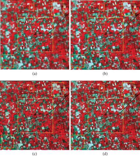
The computational time for SVR method is 16 hours per band and for the proposed method it is 4 hours per band. The proposed method predicts HR data in patchwise but the SVR method predicts pixelwise so that it takes high computational time. Therefore, our method is computationally efficient than the SVR method. The average RMSE of four bands for SVR method is 0.01 and for our method it is 0.009; it indicates that the proposed method shows a better image quality. Training and prediction were done in multiresolution domain of NSCT. The NSCT preserves the smoothness along the edges so that our method got less bias. The average SSIM of four bands for SVR method is 0.9252 and for our method it is 0.9396; the proposed method shows better structural information than the SVR method. The SSIM measures the spatial quality of the local structures in an image (Wang et al. 2004). In our method, training and prediction are patchwise and has one-pixel overlap with neighboring patches. Consequently, local structures in our method maintain a neighborhood relation with the surrounding patches. Because of these local structures, our method got high SSIM than SVR method. The proposed method has less spectral distortion than SVR method with reference to the SAM values shown in Table 2.

Table 2. Quantitative comparison between predicted and actual reflectance for the experimental data-set: 1.

Method	Computational time (in hours per band)	SSIM				RMSE				SAM
		B2	B3	B4	B5	B2	B3	B4	B5
CCL (proposed method)	4	0.9494	0.9344	0.9255	0.9494	0.0062	0.0108	0.0120	0.0071	1.8753
SVR (Zhang and Huang 2013)	16	0.9385	0.9250	0.9058	0.9316	0.0069	0.0118	0.01309	0.0084	1.8942

Note: Bold indicates the proposed method is superior in every quality parameter of the Table 2 when compared to an SVR method.

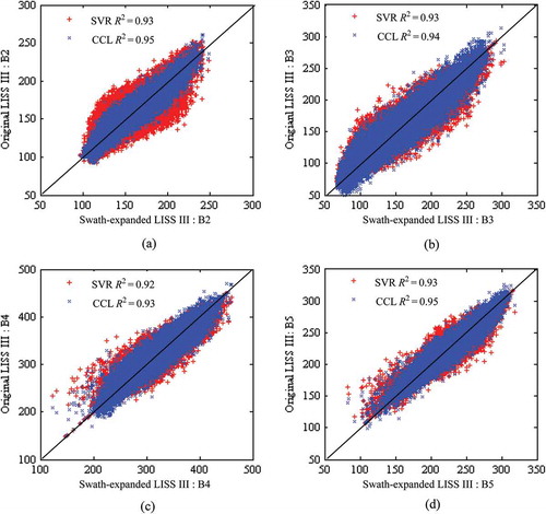
The scatter plots of the predicted against those of the original images for each band are shown in Figure 6(a)–(d). They provide an intuitive comparison between the estimated and actual reflectance on the approximation extent of distribution. These figures clearly distinguished the prediction accuracy of our method against the SVR. Blue color points in Figure 6(a)–(d) correspond to the proposed CCL method, and most of them are converged toward the 1:1 line than the red color points of the SVR method. Some of the red color points of the SVR method are diverged away from the 1:1 line. This divergence from the 1:1 contributes high error. An average of the four bands for the SVR is 0.9275 and for our method it is 0.9425. It indicates the proposed CCL method predicts more accurately than the SVR method.

Figure 6. Scatter plots between the predicted and actual reflectance values of SVR and the proposed CCL methods (where scale factor is 1000).

The yellow color box at the center of the Figure 5(a)–(d) represents the overlapping region of the LISS III and AWiFS. The small yellow color boxes in the nonoverlapping region of Figure 5(c) show the some of the patches that are showing a noticeable sharpness than the patches in Figure 5(b). This visual comparison shows that the proposed CCL method outperforms the SVR in prediction of the high-spatial-resolution image.

4.2. Experimental data-set: 2

In this experiment, we have used the crop lands area nearby Abohar of Punjab in India. This data-set contains vegetation lands, wetlands, bare soil and small water bodies in both the overlapping and nonoverlapping regions of AWiFS and LISS III images. The overlapped LISS III on the full AWiFS scene is shown in yellow color box in Figure 7(a). Figure 7(b) is swath-expanded LISS III with SVR method. Figure 7(c) is swath-expanded LISS III with the proposed CCL method. Figure 7(d) is the corresponding original LISS III image.

Figure 7. Swath-expanded LISS III (in green-red-NIR false color composition) using SVR and the proposed CCL. (a) LISS III overlapped at the center of full AWiFS scene (input image). (b) Swath-expanded LISS III using SVR Zhang and Huang (2013) method. (c) Swath-expanded LISS III using CCL (proposed method). (d) Original LISS III.

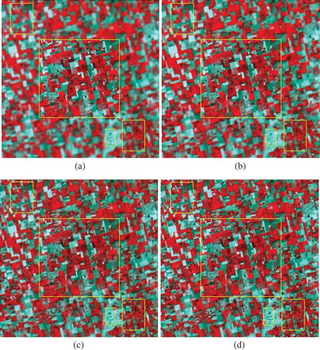
The average RMSE of four bands for SVR method is 0.0106 and for our method it is 0.0093; it indicates that the proposed method shows a better image quality. The average SSIM of four bands for SVR method is 0.9236 and for our method it is 0.9442; the proposed method shows better structural information than the SVR method. The proposed method has less spectral distortion than SVR method with reference to the SAM values shown in Table 3.

Table 3. Quantitative comparison between predicted and actual reflectance for the experimental data-set: 2.

Method	Computational time (in hours per band)	SSIM				RMSE				SAM
		B2	B3	B4	B5	B2	B3	B4	B5
CCL (proposed method)	4	0.9508	0.9418	0.9325	0.9519	0.0064	0.0113	0.0125	0.0071	1.4786
SVR (Zhang and Huang 2013)	16	0.9346	0.9217	0.9076	0.9308	0.0074	0.0127	0.0141	0.0082	1.5251

Note: Bold indicates the proposed method is superior in every quality parameter of the Table 3 when compared to an SVR method.

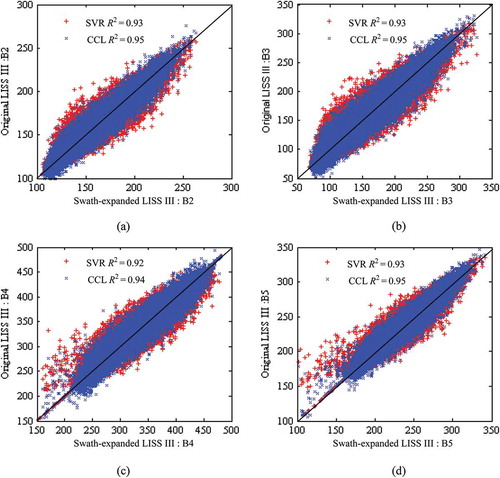
The scatter plots of the experimental data-set 2 for each band are shown in Figure 8(a)–(d). These figures clearly distinguished the prediction accuracy of our method against the SVR. Blue color points in Figure 8(a)–(d) correspond to the proposed CCL method, and most of them are converged toward the 1:1 line than the red color points of the SVR method. Some of the red color points of the SVR method are diverged away from the 1:1 line. This divergence from the 1:1 contributes high error. An average of the four bands for the SVR is 0.9275 and for our method it is 0.9475. It indicates the proposed CCL method predicts more accurately than the SVR method.

Figure 8. Scatter plots between predicted and actual reflectance values of SVR and the proposed CCL methods (where scale factor is 1000).

The yellow color box at the center of the Figure 7(a)–(d) represents the overlapping region of the LISS III and AWiFS. The small yellow color boxes in the nonoverlapping region of Figure 7(c) show the some of the patches that are showing a noticeable sharpness than the patches in Figure 7(b). This visual comparison shows that the proposed CCL method outperforms the SVR in prediction of the high-spatial-resolution images.

5. Discussion

The 740-km swath is acquired with two different sensors (ISRO 2012). First 370-km swath is acquired with AWiFS-A sensor, and the next 370-km swath is acquired with AWiFS-B sensor. The radiometric differences for both the sensors AWiFS-A and AWiFS-B can be normalized. There is no atmospheric, solar illumination and viewing angle differences for the overlapping regions of AWiFS and LISS III images in simultaneous acquisition. Although both the AWiFS and LISS III sensors acquire the data in the same spectral bandwidths, they contain different relative spectral response (RSR) curves as shown in Figure 9. The differences such as solar illumination angle and satellite viewing angle, which are occurred in the nonoverlapping region with respect to the overlapping region, and RSR differences can be normalized with techniques described in the Table 4 before applying the proposed method to the original data-sets. In Table 4, we described the possibility to correct the bidirectional reflectance distribution function (BRDF) effects in the nonoverlapping region (Walthall et al. 1985; Goward et al. 2012; Srivastava et al. 2014). In our experiments, to avoid the radiometric, BRDF, spectral and geometric differences, we created a simulated AWiFS image by degrading the original LISS III. We evaluated the effect of the proposed method with the simulated AWiFS and the original LISS III. The output of both CCL and SVR methods is validated with the original LISS III images.

Figure 9. Relative spectral response (RSR) of Resourcesat-2 AWiFS and LISS III sensors.

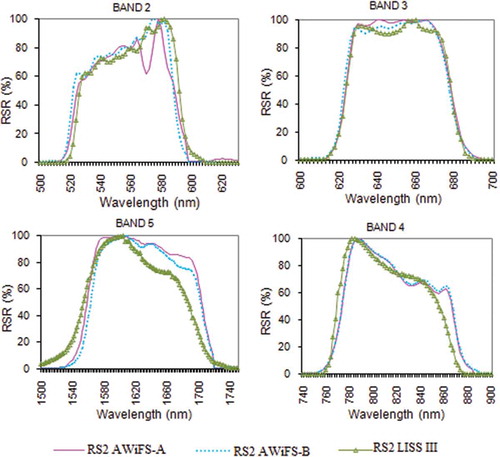
Table 4. Techniques to normalize the differences between AWiFS and LISS III sensor data.

Difference	Techniques to reduce the difference
Atmospheric effect	AWiFS and LISS III images have similar atmospheric effects in the overlapping region because they are acquired at the same time.
Sun elevation angle Sun azimuth angle Sensor elevation angle Sensor azimuth angle	Because the images of AWiFS sensor are across ± 24.3° from nadir, its overlapping and nonoverlapping regions with LISS III have the potential of being impacted by bidirectional reflectance distribution function (BRDF) phenomena. These BRDF biases can be corrected with reflectance correction factor with respect to the view zenith angle (Walthall et al. 1985; Goward et al. 2012; Srivastava et al. 2014).
Spectral bandwidth	Although AWiFS and LISS III sensors have same spectral bandwidths, they have different relative spectral response (RSR) as shown in Figure 9. So the AWiFS reflectance was normalized to LISS III reflectance by the procedure described in Chander, Coan, and Scaramuzza (2008).
Spatial resolution	The nonoverlapping region of AWiFS with LISS III is enhanced to LISS III spatial resolution using CCL (proposed method).

6. Conclusion

Swath expansion through spatial resolution enhancement was investigated. The 140-km swath of LISS III overlaps with the 740-km swath of AWiFS at center portion in simultaneous acquisition. We assumed that the nonoverlapping region of AWiFS contains similar Earth’s surface features of the overlapping region. With this assumption, spatial resolution of the nonoverlapping region of AWiFS is enhanced to the spatial resolution of LISS III using single-image super-resolution technique. Single-image super-resolution requires a prior knowledge about the desired HR image. Although, in our method, prior knowledge is limited to the overlapping region of AWiFS and LISS III, the desired LISS III patch is predicted more accurately than SVR.

Zhang and Huang (2013) recently proposed spatial resolution enhancement through a single-image super-resolution technique. It uses SVR to predict HR pixels from LR patches. Zhang and Huang (2013) prediction process is pixelwise so that it takes more computational time to predict full image and not to maintain a neighborhood relationship with the surrounding pixels. But our prediction process is patchwise. Hence, it took less computational time and maintains neighborhood relationship.

The proposed method can create a synthetic image at 740-km swath, spatial and 5-day temporal repetition. Spaceborne sensors have limited capability to acquire images with wider swath at high spatial and high temporal resolution simultaneously. Our method facilitates an alternative approach to get such images. We investigated effect of the proposed method with two experimental data-sets. These two experiments demonstrated that the proposed method outperforms the SVR-based method in quantitative and qualitative comparisons. Although our method is four times faster than the Zhang and Huang (2013) method, till there is a need to improve the computational efficiency for larger study areas. Future work of this article is to minimizing computational time and improving the prediction accuracy.

Disclosure statement

No potential conflict of interest was reported by the author(s).

Additional information

Funding

This research was supported under Technology Development Project (TDP) at National Remote Sensing Centre, ISRO, Department of Space, Government of India [project code 0606313AE901].

References

- Auernhammer, H. 2001. “Precision Farming—The Environmental Challenge.” Computers and Electronics in Agriculture 30: 31–43. doi:10.1016/S0168-1699(00)00153-8.
- Baker, S., and T. Kanade. 2002. “Limits on Super-Resolution and How to Break Them.” IEEE Transactions on Pattern Analysis and Machine Intelligence 24: 1167–1183. doi:10.1109/TPAMI.2002.1033210.
- Chander, G., M. J. Coan, and P. L. Scaramuzza. 2008. “Evaluation and Comparison of the IRS-P6 and the Landsat Sensors.” IEEE Transactions on Geoscience and Remote Sensing 46: 209–221. doi:10.1109/TGRS.2007.907426.
- Chang, C. C., and C. J. Lin. 2001. “LIBSVM: A Library for Support Vector Machines.” Accessed 30 June, 2014. http://www.csie.ntu.edu.tw/~cjlin/libsvm.
- Chang, H., D. Y. Yeung, and Y. Xiong. 2004. “Super-Resolution through Neighbor Embedding.” Proceedings IEEE Conference CVPR 1: I-275–I-282.
- Coops, N. C., M. Johnson, M. A. Wulder, and J. C. White. 2006. “Assessment of QuickBird High Spatial Resolution Imagery to Detect Red Attack Damage Due to Mountain Pine Beetle Infestation.” Remote Sensing of Environment 103: 67–80. doi:10.1016/j.rse.2006.03.012.
- Da Cunha, A. L., J. Zhou, and M. N. Do. 2006. “The Nonsubsampled Contourlet Transform: Theory, Design, and Applications.” IEEE Transactions on Image Processing 15: 3089–3101. doi:10.1109/TIP.2006.877507.
- Do, M. N., and M. Vetterli. 2005. “The Contourlet Transform: An Efficient Directional Multiresolution Image Representation.” IEEE Transactions on Image Processing 14: 2091–2106. doi:10.1109/TIP.2005.859376.
- Drucker, H., C. J. C. Burges, L. Kauffman, A. Smola, and V. Vapnik. 1997. “Support Vector Regression Machines.” In Neural Information Processing Systems 9, edited by M. C. Mozer, J. I. Joradn, and T. Petsche, 155–161. Cambridge, MA: MIT Press.
- Elad, M., and D. Datsenko. 2009. “Example-Based Regularization Deployed to Super-Resolution Reconstruction of a Single Image.” The Computer Journal 52: 15–30. doi:10.1093/comjnl/bxm008.
- Freeman, W. T., T. R. Jones, and E. C. Pasztor. 2002. “Example-Based Superresolution.” IEEE Computer Graphics and Applications 22: 56–65. doi:10.1109/38.988747.
- Gillespie, T. W., G. M. Foody, D. Rocchini, A. P. Giorgi, and S. Saatchi. 2008. “Measuring and Modelling Biodiversity from Space.” Progress in Physical Geography 32: 203–221. doi:10.1177/0309133308093606.
- Goward, S. N., G. Chander, M. Pagnutti, A. Marx, R. Ryan, N. Thomas, and R. Tetrault. 2012. “Complementarity of Resourcesat-1 AWiFS and Landsat TM/ETM+ Sensors.” Remote Sensing of Environment 123: 41–56. doi:10.1016/j.rse.2012.03.002.
- Güneralp, I., A. M. Filippi, and B. U. Hales. 2013. “River-Flow Boundary Delineation from Digital Aerial Photography and Ancillary Images Using Support Vector Machines.” GIScience & Remote Sensing 50 (1): 1–25.
- Hu, J., and S. Li. 2012. “The Multiscale Directional Bilateral Filter and Its Application to Multisensor Image Fusion.” Information Fusion 13: 196–206. doi:10.1016/j.inffus.2011.01.002.
- Ishak, A. M., R. Remesan, P. K. Srivastava, T. Islam, and D. Han. 2013. “Error Correction Modelling of Wind Speed through Hydro-Meteorological Parameters and Mesoscale Model: A Hybrid Approach.” Water Resources Management 27 (1): 1–23. doi:10.1007/s11269-012-0130-1.
- Islam, T., P. K. Srivastava, M. Gupta, X. Zhu, and S. Mukherjee. eds. 2014. Computational Intelligence Techniques in Earth and Environmental Sciences, 281. Dordrecht: Springer.
- ISRO. 2012. “Annual Report.” Accessed 13 May, 2014 www.isro.org/pdf/AnnuaReport2012.pdf
- Jiji, C. V., and S. Chaudhuri. 2006. “Single-Frame Image Super-Resolution through Contourlet Learning.” EURASIP Journal on Applied Signal Processing 2006: 235–235.
- Jiji, C. V., M. V. Joshi, and S. Chaudhuri. 2004. “Single‐Frame Image Super‐Resolution Using Learned Wavelet Coefficients.” International Journal of Imaging Systems and Technology 14: 105–112. doi:10.1002/ima.20013.
- Kerr, J. T., and M. Ostrovsky. 2003. “From Space to Species: Ecological Applications for Remote Sensing.” Trends in Ecology and Evolution 18: 299–305. doi:10.1016/S0169-5347(03)00071-5.
- Kim, K. I., D. H. Kim, and J. H. Kim. 2004. “Example-Based Learning for Image Super-Resolution,” In Proc. 3rd Tsinghua-KAIST Joint Workshop Pattern Recognition, Beijing, December 16–17, 140–148.
- Kim, K. I., and Y. Kwon. 2010. “Single-Image Super-Resolution Using Sparse Regression and Natural Image Prior.” IEEE Transactions on Pattern Analysis and Machine Intelligence 32: 1127–1133. doi:10.1109/TPAMI.2010.25.
- Kim, Y. H., J. Im, H. K. Ha, J. K. Choi, and S. Ha. 2014. “Machine Learning Approaches to Coastal Water Quality Monitoring Using GOCI Satellite Data.” GIScience & Remote Sensing 51 (2): 158–174.
- La Rosa, D., and D. Wiesmann. 2013. “Land Cover and Impervious Surface Extraction Using Parametric and Non-Parametric Algorithms from the Open-Source Software R: An Application to Sustainable Urban Planning in Sicily.” GIScience & Remote Sensing 50 (2): 231–250.
- Li, M., J. Im, and C. Beier. 2013. “Machine Learning Approaches for Forest Classification and Change Analysis Using Multi-Temporal Landsat TM Images over Huntington Wildlife Forest.” GIScience & Remote Sensing 50 (4): 361–384.
- Li, S., B. Yang, and J. Hu. 2011. “Performance Comparison of Different Multi-Resolution Transforms for Image Fusion.” Information Fusion 12 (2): 74–84. doi:10.1016/j.inffus.2010.03.002.
- Loew, A., R. Ludwig, and W. Mauser. 2006. “Derivation of Surface Soil Moisture from ENVISAT ASAR Wide Swath and Image Mode Data in Agricultural Areas.” IEEE Transactions on Geoscience and Remote Sensing 44: 889–899. doi:10.1109/TGRS.2005.863858.
- Milanfar, P., ed. 2010. Super-Resolution Imaging. Boca Raton, FL: CRC Press.
- Ni, K., and T. Q. Nguyen. 2007. “Image Superresolution Using Support Vector Regression.” IEEE Transactions on Image Processing 16: 1596–1610. doi:10.1109/TIP.2007.896644.
- Sanyal, J., and X. X. Lu. 2004. “Application of Remote Sensing in Flood Management with Special Reference to Monsoon Asia: A Review.” Natural Hazards 33: 283–301. doi:10.1023/B:NHAZ.0000037035.65105.95.
- Srivastava, P. K., D. Han, M. R. Ramirez, and T. Islam. 2013. “Machine Learning Techniques for Downscaling SMOS Satellite Soil Moisture Using MODIS Land Surface Temperature for Hydrological Application.” Water Resources Management 27 (8): 3127–3144. doi:10.1007/s11269-013-0337-9.
- Srivastava, P. K., D. Han, M. A. Rico-Ramirez, M. Bray, T. Islam, M. Gupta, and Q. Dai. 2014. “Estimation of Land Surface Temperature from Atmospherically Corrected LANDSAT TM Image Using 6S and NCEP Global Reanalysis Product.” Environmental Earth Sciences. doi:10.1007/s12665-014-3388-1.
- Walthall, C. L., J. M. Norman, J. M. Welles, G. Campbell, and B. L. Blad. 1985. “Simple Equation to Approximate the Bidirectional Reflectance from Vegetative Canopies and Bare Soil Surfaces.” Applied Optics 24: 383–387. doi:10.1364/AO.24.000383.
- Wang, Z., A. C. Bovik, H. R. Sheikh, and E. P. Simoncelli. 2004. “Image Quality Assessment: From Error Visibility to Structural Similarity.” IEEE Transactions on Image Processing 13 (4): 600–612. doi:10.1109/TIP.2003.819861.
- Zhang, H., and B. Huang. 2013. “Support Vector Regression-Based Downscaling for Intercalibration of Multiresolution Satellite Images.” IEEE Transactions on Geoscience and Remote Sensing 51: 1114–1123. doi:10.1109/TGRS.2013.2243736.