A comprehensive interferometric process for monitoring land deformation using ASAR and PALSAR satellite interferometric data

Abstract

This study was conducted to apply the enhanced differential interferometric process to interferometric data obtained from C-band Advanced Synthetic Aperture Radar (ASAR) and Phased Array type L-Band Synthetic Aperture Radar (PALSAR) systems, in the Marand plain, Iran. In advance, the capability of each sensor was examined with regard to the signal coherency for sensor–target interactions, which emphasized on the terrific excellency of PALSAR (L-band) to ASAR (C-band) measurements in study area. In the interferometric process, in addition to resolving the topography and baseline related errors (which is conventional in the standard D-InSAR process), subtle quantitative methods were outlined to minimize the secondary, but momentous errors (i.e., orbital and atmospheric) from differential phases. Subsequently, based on the outlined process, the mean deformation as well as three-dimensional displacement maps (using ascending and descending modes) were generated. The deformation maps significantly indicated the downward motion of the surface with the maximum rate of −0.5 millimetre per day for the period, i.e., from 2004 to 2010, with relative dominance in eastern and central to northern parts of the Marand plain. Finally, the results were validated and the source of deformation was inspected using field data such as seismic history; changes in piezometric levels and cross-checking the results from radar measurements itself.

Keywords:

• radar
• interferometry
• deformation
• ASAR
• PALSAR

1. Introduction

The Interferometric Synthetic Aperture Radar (InSAR) employs pairs of high-resolution radar images to generate excellent digital elevation maps using the phase interferometry method. Generally, exploration of land displacement can be directly detected by Global Positioning Satellite (GPS) measurement, levelling data and Satellite Interferometry methods. In any event, InSAR is suited to measure the spatial extent and magnitude of surface deformation and is less expensive than obtaining sparse point measurement (GPS surveys and levelling data); also, it can provide millions of data points in a region of about 10,000 km² (Yelizavetin and Ksenofontov 1996). An enhanced method of InSAR, i.e. D(Differential)-InSAR, was introduced and applied (Massonnet et al. 1993; Zebker et al. 1994; Galloway et al. 1998; Berardino et al. 2002; Colesanti et al. 2001; Chen et al. 2010) to measure the small change or variation, which may occur in the land surface over time. Since the first description of D-InSAR (Gabriel, Goldstein, and Zebker 1989), several scientists have successfully used this technique for monitoring land displacement related to aquifer systems (Galloway et al. 1998; Amelung et al. 2000; Hoffmann et al. 2001; Chatterjee et al. 2006; Motagh et al. 2007; Dehghani et al. 2009; Sharifikia 2011). In addition to other environmental applications of spaceborne radars for monitoring the atmosphere, land and ocean systems (Gens 2008), D-InSAR specifically has become a main key and novel tool for conducting many kinds of disaster monitoring, such as ground surface movement caused by both natural hazards (seismic activity, volcano eruption and landslides) and manmade activities (mining and groundwater extraction). Meanwhile, many spaceborne SAR satellites like ERS-1&2, Envisat-ASAR (now replaced with Sentinel 1A-ASAR), RADARSAT-1&2 and ALOS-PALSAR (now replaced with ALOS-2-PALSAR) have progressed worldwide. Moreover, fantastic developments in spatial resolution (below 1 metre) for new spaceborne SAR like German TerraSAR-X and Italian Cosmo-SkyMed constellation, along with noticeable development in Unmanned Aerial Vehicle Systems (UAVs) carrying SAR sensors, have provided the unique opportunity to easily conduct, disaster monitoring any time for various scales (regional to local) around the world (Shahbazi, Théau, and Ménard 2014)

Land subsidence can be defined as the differential sinking of the ground surface with respect to the surrounding terrain or the sea level. It can be formed by natural (e.g. tectonic motion and rise in the sea level) or man-induced (withdrawal of groundwater, oil and gas, underground fire, mineral extraction, tunnel excavation, etc.) causes. The impact of land subsidence is usually observed as a series of disastrous events such as damage to underground utility infrastructure and cracking of buildings’ lines, seawater intrusion and flood, which consequently lead to huge economic losses (Hu et al. 2004; Chatterjee et al. 2006; Phienwej, Giao, and Nutalaya 2006; Ovando-Shelley, Ossa, and Romo 2007). Because of the expansive distribution of land subsidence and its severe consequence on the environment and economy, the land subsidence has become one of the significant subjects, which needs research and technology transfer at the international level. In 1965, the United Nations Educational, Scientific, and Cultural Organization (UNESCO) adapted land subsidence as one of the major schemes for research and development (UNESCO 1970). Since then, a great number of scientists, researchers and engineers have made tremendous attempts to investigate several relevant subjects (i.e. detection, modelling and remediation) on land subsidence.

Various complicated and even more precise techniques, like Permanent Scatterer (so-called PS) or time series-based methods, were developed since the introduction of the D-InSAR technique (see Kampes [2006]; Mouélic et al. [2005]; Mora, Mallorqui, and Broquetas [2003]; Arnaud et al. [2003]). Although the new algorithms are quite more precise and effective especially for low coherency areas, they are not operationally applicable for all interested areas over the globe. Generally, these algorithms try to resolve the errors (topography, baseline, orbital and atmospheric) from the differential phase through estimation along the time span by increasing the total number of SAR observations. They demand a great number of SAR observations (usually more than 10) and the process involved is costly, so for the areas for which a few number of SAR observations are available, implementation of the standard D-InSAR technique is still a promising approach for deformation monitoring. However, care must be taken when using the conventional D-InSAR method, because there is a tendency to underestimate or even neglect the errors, which contributed to the measured phase, especially for orbital and atmospheric artefacts. Therefore, there is a need to outline a new procedure, in order to estimate all errors contributing to the differential phases while using the D-InSAR configuration and having a limited number of SAR data. Hence, the present research dealt with land subsidence monitoring in the Marand plain with an enhanced D-InSAR configuration outlined to estimate all errors contributing to differential phases and production of reliable deformation products (mean and three-dimensional subsidence map) from a limited number of SAR observations. Due to sparsely vegetative nature of the study area, two different frequencies of SAR observations (C & L band) were utilized for comparison and validation of results in this article.

2. Materials and method

2.1. Study area

The Marand plain is located in the northwest of Iran, next to the famous endangered Urmia Lake at a latitude of 38° 15ʹ to 38° 45ʹ and a longitude of 45° 00ʹ to 45° 15ʹ (see Figure 1). The elevation varies between 900 and 1300 metre and the area is surrounded by two major high ridges from north and south, i.e. Misho-Dagh and Qarah-Dagh, respectively. The mean rainfall, which is annually distributed over the land, is 300 mm.

Figure 1. Location of the study area on the shaded digital elevation map for the Marand plain (lower left) and the geological map (see the Appendix for different acronyms) of the study area (centre).

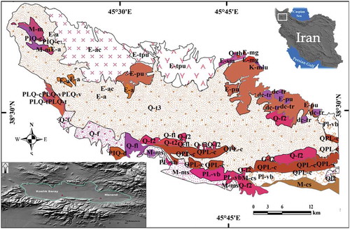
From the geological point of view (see Figure 1 and Appendix), the studied area is a part of northwestern mountain ridges in Iran, consisting of late Precambrian sedimentary to Eocene volcanic rocks (mainly andesite basalt and locally tuff). It is marked by a number of active faults oriented in the northwest and northeast–southwest directions. Mishoo is a major northwest–southeast fault trending in the south of the area, which is marked as the western part of the Tabriz active fault. Various litho-units of the area were extracted in this research based on four geology maps namely Marand, Jolfa, Tasooj and Qarah-ziaoddine provided by the Geological Survey of Iran (GSI). Digital analyses of these maps over the GIS platform indicated that various litho-unit types covered the Marand plain and its surrounding area. The sediment layer with a depth of about 1000 m covered the bottom of the plane overlying with Conglomerate and Andesite rocks. Units of volcanic rocks belonging to Eocene aligned with sedimentary rocks such as conglomerate and locally limestone cane are found to exist along the plain border in south, north and east. The coarse texture of alluvial deposition in the plain mainly resulted from rock erosion, which has hosted the main groundwater sources of the plain.

Even the Marand plain had groundwater potency, especially along the alluvial fans, but, excessive use of groundwater without any regulation has declined its level. The consequence of this situation in other plains located next to Urmia Lake’s basin along with construction of numerous dams has contributed to a recent national/international environmental disaster in the Urmia Lake and it already lost ~80% of its water coverage. Accordingly, there was a robust justification for monitoring land deformation in the Marand plain and determining its rates, sources and spatial distribution prior to any disaster remediation or risk reduction.

In this study, a comprehensive and precise D-InSAR process was performed on SAR data using two different sensors ASAR (Advanced Synthetic Aperture Radar) and PALSAR (Phased Array type L-Band Synthetic Aperture Radar) (see Figure 2). The justification behind the selection of these two different frequency radars can be first related to the characteristics of the study area, especially with regard to vegetation covers. Although, ASAR data are lonely able to provide a displacement rate, which is even more precise than that provided by PALSAR data (due to higher frequency), but because of losing the coherency in vegetated areas, the displacement map is less qualified than PALSAR ones. On the other hand, due to the lack of in situ and direct measurement of the displacement magnitude (such as extensometer or levelling networks) in the Marand plain, taking advantage of two different frequencies of radar data for self-validation of results could be the second justification. A brief, but concise description of steps which involved in the process is outlined in Sections 2.2 and 2.3.

Figure 2. The diagram for whole data processing steps.

2.2. Standard D-InSAR process

The SAR interferogram is a phase difference image, which is formed by two single look complex (SLC) images with precise registration and the interferometric process. The total differential phase difference (Δφ) can be represented by fringes for topography (φ_topo), baseline (orbital fringe, φ_orbit) and movement (φ_mov) due to the events, such as seismic or aseismic activities, groundwater, oil and gas extraction, mine exploration, and fringes from the atmospheric effect (φ_atmos) and phase noise (φ_noise). This contribution can be expressed as (Zebker et al. 1994; Rocca, Prati, and Ferretti 1997; Hanssen 2001; Mora, Mallorqui, and Broquetas 2003):

(1)

where n is an integer value, which represents the number of phase cycles in the wrapped phase difference (Δφ).

Or (Prati, Ferretti, and Perissin 2008; Ferretti et al. 2007),

(2)

Equation (2) is a detailed formulation of Equation (1) with preserving the same meaning; where h is the relative ground elevation of targets referred to a horizontal reference plane, s is the relative slant range position of targets, d is the projection along the line of sight (LOS) of the relative displacement of targets, B_n is the perpendicular baseline, R is SAR – target distance, and θ is the ‘off-nadir’ angle of the LOS. The deformation measured by this technique is aligned in the line of sight of the radar beam (LOS) and is, in fact, a resultant vector for the surface displacement in horizontal and vertical directions (Massonnet et al. 1993) and (Zebker et al. 1994).

Generation of an interferogram is possible when ground reflectivity is acquired with at least two antennae overlaps. When the perpendicular component of the baseline increases beyond a limit known as the critical baseline, no phase information is conserved, coherency is lost and interferometry is not possible. In terms of incidence angle Ψ and the critical baseline length orthogonal to the LOS of the radar, which is an important dimension, the result would be (Zebker and Villasenor 1992):

(3)

where λ is the wavelength, R is the range distance, δy is the pixel spacing in the range, and Ψ is the grazing angle. In case the radar is in the bistatic mode, p = 2, and when it is in the monostatic mode, p = 1. In fact, the baseline value with respect to the critical baseline and the Doppler Centroid Difference (DCD) between master and slave acquisitions compared with Pulse Repetition Frequency (PRF) of radar systems are important factors for selecting appropriate pairs for interferometric processing. In case the DCD is higher than the PRF, the SAR pair is not suitable for interferometry.

Accordingly, a total of 11 ASAR images were taken over the study area from June 2004 to February 2009. The images were acquired in the image mode single look complex (IMS) mode in both ascending (7 images) and descending (4 images) orbits (see Table 1). In addition to ASAR data, a total of six PALSAR images in the level-0 product in the FBD (Fine Beam Double) polarization mode acquired from June 2007 to September 2009 were used for the generation of interferograms (see Table 2).

Table 1. Interferometric pairs for ASAR data. B_p, B_cr, θ and T indicate the perpendicular, critical, incidence angles and the temporal baseline, respectively.

Pairs	Date (master)	Date (slave)	Bp (metre)	Bcr (metre)	T (day)	θ	Orbital heading
1	18 June 2004	23 July 2004	43.83	932	35	23	Ascending
2	18 June 2004	3 June 2005	42.04	932	350	23	Ascending
3	3 June 2005	9 January 2006	55.66	932	216	23	Ascending
4	20 March 2007	4 March 2008	24.60	2160	350	41	Ascending
5	4 March 2008	2 February 2009	160.25	2160	335	41	Ascending
6	16 March 2005	25 May 2005	462.71	933	70	23	Descending
7	1 March 2006	1 November 2006	417.28	933	245	23	Descending
8	25 May 2005	1 March 2006	96.16	934	280	23	Descending

Table 2. Interferometric pairs for PALSAR data. B_p, B_cr, θ and T indicate the perpendicular, critical, incidence angles and the temporal baseline, respectively.

Pairs	Date (master)	Date (slave)	Bp (metre)	Bcr (metre)	T (day)	θ	Orbital heading
1	11 June 2007	28 April 2008	301.23	6539	322	39	Ascending
2	11 June 2007	16 June 2009	98.146	6539	736	39	Ascending
3	11 September 2007	1 August 2009	176.65	6537	690	39	Ascending
4	11 September 2007	16 September 2009	124.85	6537	736	39	Ascending

Interferograms are generated by multiplying each master with the complex conjugates of the respective slave. During the generation of interferograms, spectral shift and common Doppler bandwidth filtering are performed due to the range spectral shift caused by the variable SAR viewing angle on distributed targets, which enables full capturing of the potential coherence of the scene.

Topographic fringes are removed from interferograms using mosaicked conventional digital elevation data of three arc-second shuttle radar topographic mission’s digital elevation model (STRM DEM) and simulated slant range DEM using the SAR image and DEM data. The effect of the spatial baseline is removed by precise baseline calculation and, in the case of ASAR data, the parameters embedded in DORIS (Doppler Orbitography and Radio-positioning Integrated by Satellite) files were applied. Residual phase component , the so-called differential interferometric phase, is then proportional to the terrain motion component along the LOS plus atmospheric and decorrelation noise (Prati, Ferretti, and Perissin 2008):

(4)

In order to reduce the residual phase error arising from temporal or spatial-baseline decorrelation, an adaptive filter could be applied to enhance the quality of the desired phase. The interferometric coherency (γ) or interferometric correlation (see Equation (5)) is a valuable index for indicating the quality of the measured phase (Goldstein and Werner 1998):

(5)

in which E₁ and E₂ are complex echo amplitudes received in two antenna locations and the brackets represent an ensemble average. Accordingly, an adaptive filter is applied to interferograms using coherence values in the modified version (Baran et al. 2003) of Goldstein (Goldstein and Werner 1998) filtering methods.

For resolving the so-called 2π ambiguity (Reigber and Moreira 1997) in the phase of the interferogram (unwrapping process), a network-flow algorithm (Chen and Zebker 2000, 2001, 2002), which is embedded in freely source SNAPHU software, is used.

2.3. An extension to the precise D-InSAR process

In this manuscript, the precise D-InSAR process involved the elimination of other residual phases (i.e. orbital and topographic phase residue, ionospheric and tropospheric phases) from the differential phase as well as the production of three-dimensional (3-D) displacement vectors.

2.3.1. Orbital refinement

In order to correct the transformation of the unwrapped phase into height (or displacement) values, it is mandatory to estimate residual orbital errors as well as possible phase ramps (topographic residual phases), which include precise calculation of orbital and azimuthal shifts in X, Y, and Z directions along with the estimation of residual phases arising from topography or a flat earth model (Ferretti et al. 2007). For each interferogram, the phase offset was estimated based on the height value of well-distributed points (selected in flat areas with good coherencies) and appropriate polynomials. After the estimation of the phase offset (orbital and topographic residuals), the absolute unwrapped phase was achieved by subtracting from the phase of the interferograms (i.e. phase of interferograms after unwrapping).

2.3.2. Atmospheric corrections

Among different atmospheric layers, the troposphere and the ionosphere are mainly responsible for radio signal delay. Electron density in the ionosphere causes shortening of the propagation path or phase advance and the partial pressure of water vapour in the troposphere causes an increase in the observed range or phase delay (Hanssen 2001; Hanssen and Feijt 1996; Kucheryavenkova and Zakharov 2003).

The ionospheric influence on SAR signals may result in directional fluctuations in the relative sub-pixel position of azimuth pixels, which has been already reported in the literature as azimuthal streaking (Mattar and Gray 2002), as well as lengthening of the wave paths between two radar acquisitions. L-band SAR signals are less affected by temporal canopy changes than C-band signals, which could be severely affected by ionospheric heterogeneities occurring during the synthetic aperture calculation (e.g. Quegan and Lamont [1986]; Mattar and Gray [2002]). Due to the dispersive nature of the medium, the refractive index in the ionosphere depends on the inverse of the square of the employed electromagnetic frequency. As a result, L-band SAR data are more affected than C-band SAR data. The relationship can be mathematically described as (after Wegmüller et al. [2006]):

(6)

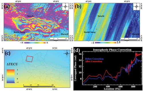
In Equation (6), λ and f are the wavelength and frequency of radar and ΔTECU is the change in the amount of TECU (Total Electron Concentration Unit) between slave and master acquisitions of SAR data. TECU values were acquired from the Centre for Orbital Determination Europe (CODE) database, which was supplied by University of Berne under the Global Ionospheric Map (GIM) project. Ionospheric streaks were detected on SAR interferograms according to the procedure proposed by Wegmüller et al. (2006). Accordingly, the ΔTECU maps were generated from the CODE database; then, the relationship between the azimuth shift (computed based on the offset tracking technique) and (calculated from Equation (6)) was examined (using regression analysis) for the areas, in which there was no evidence of displacement. According to this relationship (slope and offset of the regression), the amount of azimuth shift which was responsible only for ionospheric effects was localized and specified. Finally, after estimating the localized , the phase component of each interferogram was corrected to reduce the effect of phase advances (see Figure 3).

Figure 3. Example of ionospheric correction on SAR interferograms. Interferogram for pair No. 3 of the PALSAR data-set (a) and its respective azimuth shift map (b); the global TECU map for northwest of Iran (red and magenta rectangles show the extent of ASAR and PLASAR data, respectively) (c) and the effect of ionospheric phase correction on the respective interferogram (d).

Tropospheric-induced errors were removed using the MODIS (Moderate Resolution Imaging Spectroradiometer) cloud product (known as MOD06) obtained from the MODIS sensor on-board Terra satellite. Temperature and pressure bands of the MOD06 product were used to solve the integral equation (Equation 7) in order to calculate the incremental path length, , as (Hanssen and Feijt 1996):

(7)

In Equation (7), H is the vertical distance travelled by the SAR signal in metre, N is the refractivity (see Buck [1981] for detailed computation), θ is the incidence angle, and h is the topographic height in metre. Afterwards, the phase of each differential interferogram was separated from its module and then subtracted by the map generated from Equation (7). The resulting phase map was almost free from tropospheric-induced errors and re-combined with the module component for further processing in a complex domain.

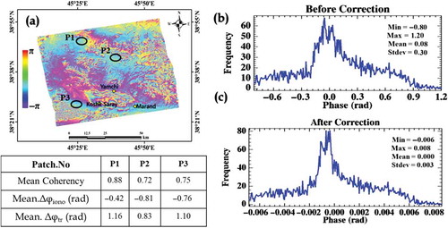
Practically, after atmospheric corrections, for those areas where there would be ‘no deformation’ between master and slave acquisitions, the phase of an interferogram should be close to zero. This is a good provision to examine the performance of the atmospheric correction method. Accordingly, a group of pixels were selected in the areas having no deformation and high coherency (>0.6), respectively. Afterwards, the phase distribution of all selected pixels were plotted to examine their distribution, both before and after atmospheric (tropospheric and ionospheric) corrections (Figure 4). As an example, by investigating the PALSAR number 3 interferogram, we observed that the phase before corrections distributed between ‘−0.8 and 1.2’ radian, while they reduced to the range of ‘−0.006 to 0.008’ radian with the mean approximately close to zero.

Figure 4. Differential interferogram for pair No. 3 of the PALSAR data-set (a), phase distribution of the respective interferogram before (b) and after (c) atmospheric corrections. Black circles in (a) indicate the three nominating patches out of the deformation areas and the table indicates the statistics related to each patch.

2.4. Phase to displacement conversions

Each 2π cycle (interferometric fringe) of the differential phase corresponds to half wavelength of displacement along with the line of sight (LOS) direction of the radar. By considering the incidence angle, LOS deformation (Δρ) can be projected onto the vertical direction; i.e. , where and λ, θ are the wavelength and mean incidence angle of the radar, respectively. In the present work, ASAR as well as PALSAR data for the C band (λ = 5.6 cm) and the L band (λ = 23.6 cm) were used. Accordingly, for each corrected absolute unwrapped phase, the vertical displacement was calculated as described above with respect to the incidence angle. In this article, an increase in the range in the case of negligible horizontal motion corresponded to subsidence and the sign convention for downward motion (subsidence) was set to negative for all the generated subsidence maps.

2.5. Geocoding

The absolute calibrated and unwrapped phase values were converted into displacement and directly geocoded into a map projection. This step was performed by considering the range-Doppler approach, which was simultaneously applied to the two antennae (Equations (8) and (9)) and the related geodetic and cartographic transformations. For each backscatter element with the corresponding estimated sensor position, the slant range and Doppler frequency were computed using range-Doppler equations (Meier, Frei, and Nuesch 1993):

(8)

(9)

where is the slant range, S and P are positions of the spacecraft and backscatter elements, and are velocities of the spacecraft and backscatter elements, is the carrier frequency, is the speed of light and is the processed Doppler frequency.

2.6. Three-dimensional decomposition of displacement vector

The ground displacement measured using the D-InSAR technique is a displacement in the line of sight (LOS) direction; i.e. range direction. As mentioned by Fialko, Simons, and Agnew (2001), the LOS vector is a resultant vector, which contains the displacement occurring in horizontal as well as vertical directions. Analytically, the measured line of sight displacement (Δρ) can be expressed as (Fialko, Simons, and Agnew 2001; Fialko 2004):

(10)

In Equation (10), θ is the incidence angle of the radar at the reflection point, V is the vertical component of displacement, α is the satellite heading vector, E and N are easting and northing components of horizontal displacement and δ_Δρ is the measurement error (e.g. due to the imprecise knowledge on satellite orbits, atmospheric delays, poor phase coherence, incorrect DEM, etc.).

In order to solve Equation (10) by compensating for the measurement error (δ_Δρ), there are mainly two unknown parameters (horizontal component (H) and vertical component (V)). By enlisting the measured LOS vectors in descending and ascending passes over the same area, two linear equations can be defined for deriving these two unknown parameters. So, for the ascending pass, this equation can be rewritten as:

(11)

And, in a similar way, the equation for the descending orbit is:

(12)

Accordingly, with respect to data availability, ascending and descending pairs of the ASAR data-set were used to calculate the horizontal and vertical displacements over the studied area. Since Equations (11) and (12) were applied to geocoded subsidence maps, the positive values in the H component indicated the eastward motion and vice versa. For the vertical component (V), the sign convention was the same as that of the LOS displacement (see Section 2.4).

3. Experiment and results

3.1. Processing results

The process which is outlined in Figure 2 was applied in each data-set of ASAR and PALSAR interferometric sets. Figure 5(a) shows an example of differential interferograms generated by ASAR pairs (pair 5). The index of signal coherency (γ), indicating the stability of the SAR signal with respect to the object along the temporal baseline, showed medium amount of coherency for almost all interferograms.

Figure 5. Examples of interferograms generated from ASAR (pair5) and PALSAR data (pair3) in the ascending mode (a and c); mean coherency map for ASAR interferograms in the ascending mode (b) and coherency map for Pair 5 of the PALSAR interferogram (d). The greyish rectangular box in (c) and (d) indicates the region of interest in which the respective coherency percentages were calculated.

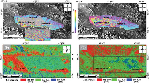
It is clear from the mean coherency map for the ASAR interferogram in Figure 5(b) that about 34% of the area had γ values of 0.00–0.33 (poor coherency), while 38% had γ values of 0.33 to 0.66 (medium coherency) and only 28% of the area had γ values more than 0.66 (strong coherency). During the process of ASAR interferograms, the result of medium to poor coherency on the ASAR data-set caused difficulties in phase unwrapping. Subjectively, for each ASAR interferogram, poor coherency areas were masked out before applying the unwrapping process. Accordingly, special care was taken for a compromise existing between the rejections of poor coherency areas (increasing quality of the differential phase) against maintaining the connectivity between high coherency patches (needed for the unwrapping process to be successful).

To address the issues of poor coherency, use of L-band radar data is preferred to C-band data in the land covers characterized by vegetation (Raucoules, Colesanti, and Carnec 2007). Accordingly, four differential interferograms were generated based on the PALSAR data-set (see Table 2). Compared with ASAR interferograms, fringes were more obvious in interferograms generated by the PALSAR data-set (see Figure 5(c)). The coherency was satisfactory (about 75% of the area had γ values more than 0.33); and also, phase discontinuities and decorrelations were significantly better than ASAR interferograms, mainly due to the fact that PALSAR images have longer wavelength and finer spatial resolution (see Figure 5(d)).

In order to calculate the average velocity deformation map in the LOS direction, a standard estimator proposed by Mouélic et al. (2005) was used:

(13)

where is the annual average displacement value (mm/year), I is the number of interferograms, is deformation values in each interferogram and is time intervals (master and slave acquisitions) in days.

Figure 6(b) and (c) shows the average deformation maps generated from PALSAR and ASAR interferograms, respectively. It is clear from the mean subsidence maps that the maximum deformation occurred in the eastern and central-northern parts of the Marand plain.

Figure 6. Site location of the study area on the ascending ASAR power image (a). Mean subsidence map for PALSAR (b) and ASAR interferograms (c); horizontal (d) and vertical components of displacement (e).

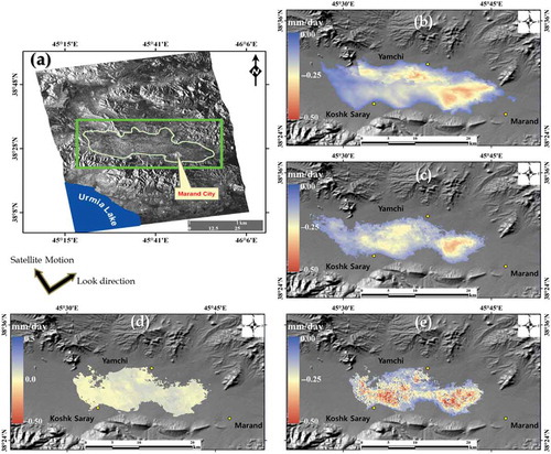
Finally, in order to extract the three-dimensional components of displacement vectors, horizontal and vertical displacements were calculated using Equations (10)–(12). Figure 6(d) and (e) demonstrates the results for horizontal and vertical displacements using data from pair 3 and pair 8 of the ASAR interferograms obtained in ascending and descending modes (see Table 1), respectively. The decomposition of the LOS vector into its horizontal and vertical components indicated the dominance of vertical displacement during the time of observations. The vertical displacement was obtained with the maximum amount of 0.5 mm per day, while the horizontal one was near zero to around 0.06 mm per day, which might be related to artificially-induced errors (the residual phase from topographic, orbital, atmospheric, or spurious phase unwrapping and satellite clock drift).

4. Validation

Land deformation in the Marand plain was mainly suspected to be generated by two mechanisms: i.e. (1) seismic activities, (2) groundwater overextraction. Compared with other influencing factors for land deformation in the Marand plain, seismic events were more suspected to be important for land subsidence after groundwater overextraction. Accordingly, the historical earthquake events were investigated in and around the plain. It was observed that, no seismic event with a magnitude of 3 or above was found to occur within 50 km radius surrounding the plain for the years between 2004 and 2010 (USGS 2010). However, the small amount of horizontal displacement (near zero) obtained from three-dimensional decomposition of the displacement vector could reject the occurrence of any fault or tectonic activities during the investigation period. Hence, it might be inferred that the seismic event and the associated downwarping of sediments could not play any significant roles in the observation period.

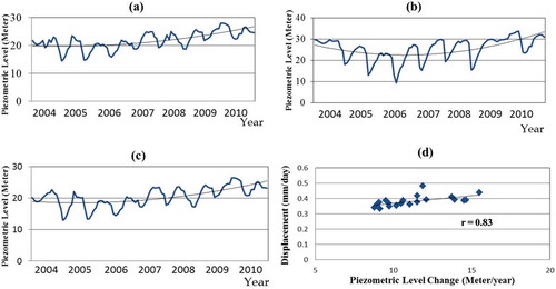
Annual accumulated precipitations are closely related to the piezometric level; and rain infiltration with irrigation overflow is the most important source for recharging the aquifers. During drought periods with low precipitation, water extraction was notably increased in both authorized as well as in illegal wells from deep aquifers, while at the same time infiltration was decreased. The consequence has been a fall in the piezometric levels, the effects of which were observed during the drought years from 2003 to 2007. Analysing the piezometer data indicated that drought led to piezometric falls of 10 to 15 m (see Figure 7(a–c)). The temporal evolution of ground deformation measured by the D-InSAR technique also showed a satisfactory correlation (r = 83%) with changes in piezometric levels of deep aquifers (see Figure 7(d)). In fact, panel (d) in Figure 7 demonstrates an acceptable relationship between the overall piezometric changes occurring during the investigation period and the spatial amount of subsidence rates. It means that the aquifers with more piezometric decline experienced a higher amount of subsidence.

Figure 7. Changes in piezometric levels during 2004–2010 in the Marand plain (a, b and c). The relationship between piezometric fall and mean displacements obtained from D-InSAR measurement over the study area (d).

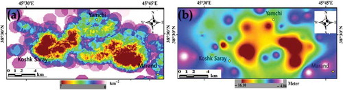
However, the only difference and bias could be related to the delay occurring between the time of the maximum piezometric fall and the emergence of subsidence. As inferred from changes in piezometric levels with deformation patterns, the deformation occurred after each de-charging of the aquifer, which was completely related to crop seasons and agricultural activities. In addition, the decline of the piezometric pressure due to groundwater withdrawal resulted in the pore pressure of the aquifer system, which intensified the striking stress over the aquifer sand layer. On the other hand, a sudden decline in the piezometric pressure due to heavy withdrawal of groundwater created hydraulic gradients between the aquifer and the overlaying restricted clay layer, which resulted in the leakage of pore water from the confining clay layer and led to inelastic compression and therefore vertical compression of the clay layer. This point became more clear in visual comparison when the coincidence between the density of pumping wells and spatial patterns of piezometric falls (see Figure 8) was noticed. The magnitude and spatial patterns of piezometric falls were highly related to the subsidence rate (Figure 7(d)), as a result, the density of the pumping wells (indication of over-exploitation of groundwater) was also related to that.

Figure 8. Inter-comparison between the density of pumping wells (number of wells per square kilometre) (a) and spatial patterns of piezometric falls during 2004 to 2010 (b).

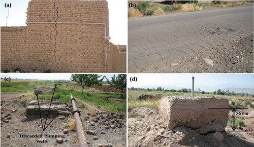
A comprehensive field campaign was conducted for finding the features related to ground subsidence. Different features like cracks on buildings and structures as well as road undulation were observed frequently along the residential areas (see Figure 9). Investigation of agricultural areas also indicated numerous casing and discards in pumping wells as well as a notable increase in the depth of drilling for groundwater extraction.

Figure 9. Subsidence evidence in the Marand plain captured during the field visit. Cracks on structures (a), crack and road undulation (b), discarded pumping wells (c) and casing in piezometric boreholes (d).

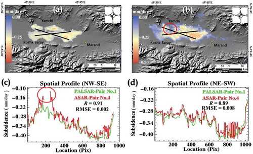
Another validation was performed by taking into account two interferometric results that were already deployed in this work. Implementing two different SAR data from two different satellites, which operated at two different frequencies, has provided the self-comparison of each radar measurement and examined the accuracy of interferometric techniques in deformation detection. Since, the capabilities of SAR measurements and differential interferometric techniques were recognized and well proved in detecting the small amount of deformation over the land, the only concern could be the accuracy of the present measurement itself. The interferogram No. 4 in the ASAR set showed the amount to be −0.42 mm per day subsidence from 20 March 2007 to 4 March 2008 while, at the same time, PALSAR interferogram No. 1 showed almost the same amount of displacement (i.e. −0.44 mm per day between 11 June 2007 and 28 April 2008). Figure 10 shows a detailed comparison between these two outcomes. The amount of correlation coefficient (R) as well as the root mean square (RMSE) for diagonal transect lines were almost promising, since correlation coefficients of 0.91 and 0.89 were shown and RMSE of 0.006 and 0.005 along NW–SE and NE–SW was indicated, respectively. The only difference (highlighted by the red circle in Figure 10) was related to signal incoherency for that particular area in the ASAR interferogram (see Figure 10(c)), while the same area was perfectly detected and mapped in the PALSAR interferogram.

Figure 10. Parity analysis between ASAR and PALSAR subsidence maps during the same temporal span. Subsidence map corresponding to PALSAR-Pair No. 1 (a) and ASAR-Pair No. 4 (b); spatial profiles related to northwest–southeast and northeast–southwest black transect lines on subsidence maps (c) and (d).

5. Conclusion and remarks

The data from two different spaceborne radar sensors, i.e. ASAR and PALSAR, were utilized in a precise and comprehensive interferometric process. The results obtained from each sensor primarily proved the occurrence of subsidence in the study area; however, they showed slightly different patterns and rates according to their system–target interactions. An ASAR interferogram was useful, especially in detecting the deformation, which occurred in a short time span (monthly); but, it was quite unable to detect deformation occurring in annual intervals. On the other hand, the L-band PALSAR data demonstrated and proved their capability to detect, first, the deformation in vegetated areas and, second, a larger amount of displacement in longer time spans. From interferometric results, different components and products such as the accumulated amount of subsidence, monthly mean rate of subsidence and three-dimensional displacement vectors were also generated.

The probable causes of land subsidence in the Marand plain were also investigated. Pieces of evidence showed the major role of overextraction of groundwater from almost coarse texture aquifers in the emergence of ground subsidence. The piezometric changes for boreholes demonstrated the piezometric reduction of about 4–6 m after each discharge period (small charging also occurred in the rainy season) and the overall piezometric fall of about 10–15 m during the time of observation, i.e. 2004–2010. The reasoning based on SAR detection was another approach for validating the interferometric results. As discussed in Section 4, the interferogram No. 4 in the ASAR data-set and interferogram No. 1 in the PALSAR data-set, which were acquired in almost the same period, showed approximately the same amount of settlement as well as spatial extent.

In summary, using two frequency SAR data instead of trying more sophisticated and costly techniques (like PS or time-series based-techniques) provided a solution for areas, in which shorter wavelength (i.e. C band) was not able to procure qualified results and, in another case, supplied an alternation for the self-validation of measurement based on the SAR process itself. However, for more understanding of the nature of subsidence, more numbers of InSAR data (might be possible with Sentinel 1-A (C-band) and future ALOS-2 (L-band) data) with reasonable temporal baselines along with other field ancillary data had to be procured and processed.

Disclosure statement

No potential conflict of interest was reported by the author(s).

Acknowledgements

The authors thank the European Space agency (ESA) for providing ASAR data and Japan Aerospace Exploration Agency (JAXA) for providing the PALSAR data-set. The authors would like to thank the East Azerbaijan Province Water Resource Organization for sharing the hydrological data of the Marand plain. They would also like to thank respected reviewers for their constructive comments.

Appendix. Acronyms and full descriptions of different types of geological units in Figure 1

Table

Geological unit	Description
Ql2	Low level terraces
dc-tr	Volcanic domes, dacite, trachydacite
E-a	Andesite
E-ac	Agglomerate tuff, conglomerate with breccia lava
E-mg	Red and green gypsiferous marl
E-pu	Pyroclastics
E-sm	Red sandstone with minor interaction of mart
E-tpu	Tuff, pyroclastics
G-f2	Young terrace and gravel fan
K-mlu	Light grey marly limestone
M-cs	Pale red consolidated feature forming conglomerate
M-m	Red and grey salutiferous and gypsiferous marl
M-ms	Red sandstone with interaction of marl
PIQ-c	Conglomerate
PIQ-d	Volcanic domes, dacite and rhyodacite
Pl-vb	Volcanic breccia
PL-vb	Volcanic breccia
PLQ-c	Conglomerate
PLQ-t	Tuff, pumice, agglomerate and conglomerate
PLQ-v	Conglomerate
Q-f	Gravel fans
Q-f2	Young terrace and gravel fan
Q-fl	Old terrace and gravel fan
Q-t2	Low lwvwl terrace
Q-t3	Gravel plain and cultivated areas
Q-th	High level terrace
Q-tr	Travertine
QPL-c	Moderately consolidated conglomerate

References

- Amelung, F., C. Oppenheimer, P. Segall, and H. Zebker. 2000. “Ground Deformation near Gada ‘Ale Volcano, Afar, Observed by Radar Interferometry.” Geophysical Research Letters 27 (19): 3093–3096. doi:10.1029/2000GL008497.
- Arnaud, A., N. Adam, R. Hanssen, J. Inglada, J. Duro, J. Closa, and M. Eineder. 2003. “ASAR ERS Interferometric Phase Continuity.” Paper presented at the International Geoscience and Remote Sensing Symposium, Toulouse, July 21–25.
- Baran, I., P. Stewart Mike, M. Kampes Bert, Z. Perski, and P. Lilly. 2003. “A Modification to the Goldstein Radar Interferogram Filter.” IEEE Transactions on Geoscience and Remote Sensing 41: 2114–2118. doi:10.1109/TGRS.2003.817212.
- Berardino, P., G. Fornaro, R. Lanari, and E. Sansosti. 2002. “A New Algorithm for Surface Deformation Monitoring Based on Small Baseline Differential SAR Interferograms.” IEEE Transactions on Geoscience and Remote Sensing 40 (11): 2375–2383. doi:10.1109/TGRS.2002.803792.
- Buck, A. L. 1981. “New Equations for Computing Vapor Pressure and Enhancement Factor.” National Center for Atmospheric Research 20: 1527–1532.
- Chatterjee, R. S., B. Fruneau, J. P. Rudant, P. S. Roy, P.-L. Frison, R. C. Lakhera, V. K. Dadhwal, and R. Saha. 2006. “Subsidence of Kolkata (Calcutta) City, India during the 1990s as Observed from Space by Differential Synthetic Aperture Radar Interferometry (D-Insar) Technique.” Remote Sensing of Environment 102 (1–2): 176–185. doi:10.1016/j.rse.2006.02.006.
- Chen, C. W., and H. A. Zebker. 2000. “Network Approaches to Two-Dimensional Phase Unwrapping: Intractability and Two New Algorithms.” Journal of the Optical Society of America A 17: 401–414. doi:10.1364/JOSAA.17.000401.
- Chen, C. W., and H. A. Zebker. 2001. “Two-Dimensional Phase Unwrapping with Use of Statistical Models for Cost Functions in Nonlinear Optimization.” Journal of the Optical Society of America A 18: 338–351. doi:10.1364/JOSAA.18.000338.
- Chen, C. W., and H. A. Zebker. 2002. “Phase Unwrapping for Large SAR Interferograms: Statistical Segmentation and Generalized Network Models.” IEEE Transactions on Geoscience and Remote Sensing 40: 1709–1719. doi:10.1109/TGRS.2002.802453.
- Chen, F., H. Lin, K. Yeung, and S. Cheng. 2010. “Detection of Slope Instability in Hong Kong Based on Multi-baseline Differential SAR Interferometry Using ALOS PALSAR Data.” GIScience & Remote Sensing 47 (2): 208–220. doi:10.2747/1548-1603.47.2.208.
- Colesanti, C., A. Ferretti, C. Prati, and F. Rocca. 2001. “Comparing GPS, Optical Leveling and Permanent Scatterers.” Paper presented at the Geoscience and Remote Sensing Symposium, IGARSS ’01, IEEE 2001 International, Sydney, July 9–13.
- Dehghani, M., M. J. V. Zoej, S. Saatchi, J. Biggs, B. Parsons, and T. Wright. 2009. “Radar Interferometry Time Series Analysis of Mashhad Subsidence.” Journal of the Indian Society of Remote Sensing 37 (1): 147–156. doi:10.1007/s12524-009-0006-x.
- Ferretti, A., A. Monti, C. Prati, and F. Rocca. 2007. InSAR Principles: Guidelines for SAR Interferometry Processing and Interpretation. Noordwijk: ESA Publications.
- Fialko, Y. 2004. “Probing the Mechanical Properties of Seismically Active Crust with Space Geodesy: Study of the Co-Seismic Deformation Due to the 1992 Mw7.3 Landers (Southern California) Earthquake.” Journal of Geophysical Research 109. doi:10.1029/2003JB002756.
- Fialko, Y., M. Simons, and D. Agnew. 2001. “The Complete (3-D) Surface Displacement Field in the Epicentral Area of the 1999 Mw 7.1 Hector Mine Earthquake, California, from Space Geodetic Observations.” Geophysical Research Letters 28 (16): 3063–3066. doi:10.1029/2001GL013174.
- Gabriel, A. K., R. M. Goldstein, and H. A. Zebker. 1989. “Mapping Small Elevation Changes over Large Areas: Differential Radar Interferometry.” Journal of Geophysical Research 94: (B7):9183-91. doi:10.1029/JB094iB07p09183.
- Galloway, D. L., K. W. Hudnut, S. E. Ingebritsen, S. P. Phillips, G. Peltzer, F. Rogez, and P. A. Rosen. 1998. “Detection of Aquifer System Compaction and Land Subsidence Using Interferometric Synthetic Aperture Radar, Antelope Valley, Mojave Desert, California.” Water Resources Research 34 (10): 2573–2585. doi:10.1029/98WR01285.
- Gens, R. 2008. “Oceanographic Applications of SAR Remote Sensing.” GIScience & Remote Sensing 45 (3): 275–305. doi:10.2747/1548-1603.45.3.275.
- Goldstein, R. M., and C. L. Werner. 1998. “Radar Interferogram Filtering for Geophysical Applications.” Geophysical Research Letters 25 (21): 4035–4038. doi:10.1029/1998GL900033.
- Hanssen, R., and A. Feijt. 1996. “A First Quantitative Evaluation of Atmospheric Effects on SAR Interferometry.” In ‘FRINGE 96ʹ Workshop on ERS SAR Interferometry, September 30–October 2. Zurich: ESA SP-406.
- Hanssen, R. F. 2001. Radar Interferometry: Data Interpretation and Error Analysis. Dordrecht: Kluwer Academic Publishers.
- Hoffmann, J., H. A. Zebker, D. L. Galloway, and F. Amelung. 2001. “Seasonal Subsidence and Rebound in Las Vegas Valley, Nevada, Observed by Synthetic Aperture Radar Interferometry.” Water Resources Research 37 (6): 1551–1566. doi:10.1029/2000WR900404.
- Hu, R. L., Z. Q. Yue, L. C. Wang, and S. J. Wang. 2004. “Review on Current Status and Challenging Issues of Land Subsidence in China.” Engineering Geology 76 (1–2): 65–77. doi:10.1016/j.enggeo.2004.06.006.
- UNESCO, and IASH. 1970. “Land Subsidence.” Paper presented at the Proceedings of the First International Symposium on Land Subsidence, Tokyo, September.
- Kampes, B. M. 2006. Radar Interferometry: Persistent Scatterer Technique. Vol. 12. Dordrecht: Springer.
- Kucheryavenkova, I. L., and A. I. Zakharov. 2003. “Use of Radar Inferometry for Study of Dynamics of the Earth’s Surface and Troposphere.” Mapping Sciences and Remote Sensing 40 (1): 29–40. doi:10.2747/0749-3878.40.1.29.
- Massonnet, D., M. Rossi, C. Carmona, F. Adragna, G. Peltzer, K. Feigl, and T. Rabaute. 1993. “The Displacement Field of the Landers Earthquake Mapped by Radar Interferometry.” Nature 364 (6433): 138–142. doi:10.1038/364138a0.
- Mattar, K. E., and A. L. Gray. 2002. “Reducing Ionospheric Electron Density Errors in Satellite Radar Interferometry Applications.” Canadian Journal of Remote Sensing 28: 593–600. doi:10.5589/m02-051.
- Meier, E., U. Frei, and D. Nuesch. 1993. “Precise Terrain Corrected Geocoded Images.” In SAR Geocoding: Data and System, edited by G. Schreier, 173–185. Karlsruhe: Herbert Wichmann Verlag GmbH.
- Mora, O., J. J. Mallorqui, and A. Broquetas. 2003. “Linear and Nonlinear Terrain Deformation Maps from a Reduced Set of Interferometric SAR Images.” IEEE Transactions on Geoscience and Remote Sensing 41 (10): 2243–2253. doi:10.1109/TGRS.2003.814657.
- Motagh, M., Y. Djamour, T. R. Walter, H.-U. Wetzel, J. Zschau, and S. Arabi. 2007. “Land Subsidence in Mashhad Valley, Northeast Iran: Results from Insar, Levelling and GPS.” Geophysical Journal International 168 (2): 518–526. doi:10.1111/j.1365-246X.2006.03246.x.
- Mouélic, L. S., D. Raucoules, C. Carnec, and C. King. 2005. “A Least Squares Adjustment of Multi-Temporal Insar Data: Application to the Ground Deformation of Paris.” Photogrammetric Engineering and Remote Sensing 71 (2): 197–204. doi:10.14358/PERS.71.2.197.
- Ovando-Shelley, E., A. Ossa, and M. P. Romo. 2007. “The Sinking of Mexico City: Its Effects on Soil Properties and Seismic Response.” Soil Dynamics and Earthquake Engineering 27 (4): 333–343. doi:10.1016/j.soildyn.2006.08.005.
- Phienwej, N., P. Giao, and P. Nutalaya. 2006. “Land Subsidence in Bangkok, Thailand.” Engineering Geology 82 (4): 187–201. doi:10.1016/j.enggeo.2005.10.004.
- Prati, C., A. Ferretti, and D. Perissin. 2008. “Recent Advances on Surface Ground Deformation Measurement by Means of Repeated Space-borne SAR Observations.” Journal of Geodynamics. doi:10.1016/j.jog.2009.10.011.
- Quegan, S., and J. Lamont. 1986. “Ionospheric and Tropospheric Effects on Synthetic Aperture Radar Performance.” International Journal of Remote Sensing 7 (n4): 525–539. doi:10.1080/01431168608954707.
- Raucoules, D., C. Colesanti, and C. Carnec. 2007. “Use of SAR Interferometry for Detecting and Assessing Ground Subsidence.” Comptes Rendus - Geoscience 339 (5): 289–302. doi:10.1016/j.crte.2007.02.002.
- Reigber, A., and J. Moreira. 1997. “Phase Unwrapping by Fusion of Local and Global Methods.” Paper presented at the Proceedings of IGARSS’97 Symposium, Singapore, August 3–8.
- Rocca, F., C. Prati, and A. Ferretti. 1997. “An Overview of ERSSAR Interferometry.” Paper presented at the Proceedings of the 3rd ERS Symposium on Space at the Service of our Environment, Florence, March 18–21.
- Shahbazi, M., J. Théau, and P. Ménard. 2014. “Recent Applications of Unmanned Aerial Imagery in Natural Resource Management.” GIScience & Remote Sensing 51 (4): 339–365. doi:10.1080/15481603.2014.926650.
- Sharifikia, M. 2011. “Land Subsidence Disaster Evaluation over Settlement Areas of Iran.” [In Persian.] Journal of Engineering Geology Scientific Research 3: 43–58.
- USGS, National Earthquake Information Center. 2010. U.S. Geological Survey Earthquake Data Base. http://eqint.cr.usgs.gov/neic/
- Wegmüller, U., C. Werner, T. Strozzi, and A. Wiesmann. 2006. “Ionospheric Electron Concentration Effects on SAR and INSAR.” Proceedings of IGARSS 2006, Denver, CO, July 31–August 4.
- Yelizavetin, I. V., and Y. A. Ksenofontov. 1996. “Precision Terrain Measurement by SAR Interferometry.” Mapping Sciences and Remote Sensing 33 (1): 1–19. doi:10.1080/07493878.1996.10642010.
- Zebker, H. A., P. A. Rosen, R. M. Goldstein, A. Gabriel, and C. L. Werner. 1994. “On the Derivation of Coseismic Displacement Fields Using Differential Radar Interferometry: The Landers Earthquake.” Journal of Geophysical Research 99: 19617–19634. doi:10.1029/94JB01179.
- Zebker, H. A., and J. Villasenor. 1992. “Decorrelation in Interferometric Radar Echoes.” IEEE Transactions on Geoscience and Remote Sensing 30 (5): 950–959. doi:10.1109/36.175330.