
Abstract
The nighttime stable light (NSL) images on board the Operational Line-scan System (OLS) of the Defense Meteorological Satellite Program (DMSP) are useful for extracting large-scale built-up urban areas. However, most NSL-based studies are presently empirical threshold-based approaches. They always overestimate the areas of built-up land in urban regions because of the ‘blooming’ effect of NSL; and overlook small patches in developing towns where the NSL is much lower. In this study, a neighborhood statistics analysis (NSA) method is developed on the basis of the relative spatial variations between neighboring built-up and non-built-up pixels in DMSP-OLS images. It is applied to extract the built-up areas of eight cities in the Pearl River Delta in 1996, 2000, 2005, and 2009. The validations indicate that the total areas of the NSA-mapped results are highly correlated with those from Landsat TM/ETM+ data (R2 = 0.94; p < 0.001). The comparison results, which are evaluated by landscape indices (the landscape shape index (LSI), the contiguity index (CONTIG), and the perimeter area ratio (PARA)), also show good correlations (R2 > 0.46; p < 0.001). In addition, the total NSL of the built-up urban areas is significantly correlated with the statistical population data (R2 = 0.62; p < 0.001), which indirectly confirms the effectiveness of our proposed method.
1. Introduction
Thirty years of rapid urbanization in China have resulted in a 3.37-fold increase in built-up areas (Fang Citation2009; Lu et al. Citation2008, Citation2012). Large amounts of natural lands in cities are being replaced by artificial surfaces, which cause numerous environmental and ecological problems (Milesi et al. Citation2003; Imhoff et al. Citation2004; Su et al. Citation2010; Chen et al. Citation2012). Therefore, accurately monitoring the regional expansion of built-up areas in China is essential (He et al. Citation2006; Liu et al. Citation2012). At present, medium- or high-resolution remote sensing methods, which are mainly based on IKONOS, Quickbird, Landsat Thematic Mapper (TM)/Enhanced Thematic Mapper plus (ETM+), and Systeme Probatoire d’Observation de la Terre (SPOT)/High Resolution Visible (HRV) images (Cao et al. Citation2009; Liu et al. Citation2012; Bhatti and Tripathia Citation2014), are commonly used. However, because of the limited geographic coverage of medium- and high-resolution images, these methods require a large number of scenes to cover the regional and national scales (Liu et al. Citation2003, Citation2005, Citation2010; Zhang, He, and Liu Citation2014).
Nighttime stable light (NSL) images on board the Operational Line-scan System (OLS) of the Defense Meteorological Satellite Program (DMSP), which uses a low-light detecting sensor to detect city night lights (Elvidge et al. Citation1997, Citation1999, Citation2001), were first demonstrated to be capable of mapping built-up urban areas by Croft (Citation1978) and Kramer (Citation1994). Subsequent studies demonstrated the superiority of DMSP-OLS NSL in extracting the built-up urban areas at global (Elvidge et al. Citation1997, Citation1999, Citation2001, Citation2007, Citation2009; Henderson et al. Citation2003; Schneider et al. Citation2003; Zhang and Seto Citation2011), national (Pandey, Joshi, and Setob Citation2013; Qi and Chopping Citation2007; Sutton et al. Citation2009; Liu et al. Citation2012; Yu et al. Citation2014; Ma et al. Citation2012; Zhou et al. Citation2014), and local scales (Imhoff et al. Citation1997a, Citation1997b; Small, Pozzi, and Elvidge Citation2005; Lu et al. Citation2008; Cao et al. Citation2009; Shi et al. Citation2014; Wei et al. Citation2014). However, most NSL-based studies presently use empirical threshold-based approaches (e.g., Imhoff et al. Citation1997a, Citation1997b; Henderson et al. Citation2003; Milesi et al. Citation2003). These NSL-based approaches are different from the medium- and high-resolution methods that detect ground objects based on the relative reflections of solar radiation (Liu et al. Citation2012). In comparison, they set empirical thresholds to extract built-up urban areas of different sizes and NSL intensities. Therefore, the threshold methods not only overestimate the built-up area in urban regions because of ‘blooming’ NSL but also miss small patches of built-up lands in developing towns, where the NSL is much lower (e.g., Imhoff et al. Citation1997a; Owen Citation1998; Sutton et al. Citation2001; Lawrence et al. Citation2002; Henderson et al. Citation2003; Small, Pozzi, and Elvidge Citation2005; Cao et al. Citation2009).
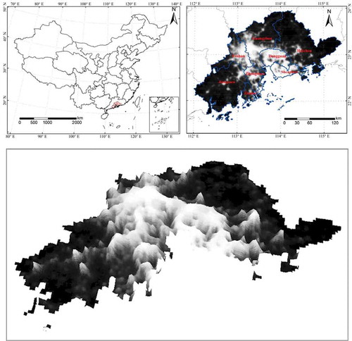
The hypothesis of our proposed method is inspired by the similarities between DMSP-OLS NSL and DEM images. The three-dimensional patterns of NSL images are similar to the three-dimensional terrain (). The pixel DN values of built-up areas in DMSP-OLS NSL images are relatively higher than those of neighboring non-built-up areas. Identifying the demarcation line between the two land cover types is equivalent to distinguishing the built-up areas from the non-built-up areas. Because topographic maps can clearly reveal terrain variations, such as ridges and valleys, the demarcation lines between built-up areas and non-built-up areas could be identified by analyzing the topographic maps of DMSP-OLS NSL images. Therefore, this article applies the neighborhood statistics analysis (NSA) method (Angelelli et al. Citation2011; Appendix 1) to generate topographic maps from DMSP-OLS NSL images and extract the built-up areas of the Pearl River Delta from 1996 to 2009. Multitemporal NSL images and quasi-geostationary Landsat TM/ETM+ images are used to evaluate the proposed method. The results are further compared with those mapped by the global-fixed and local-optimized threshold methods. The global-fixed threshold method uses an identical NSL value to classify built-up urban areas of all cities by closely matching the targeted total area, while the local-optimized threshold method assigns one optimal DN threshold for each city (Imhoff et al. Citation1997a; Milesi et al. Citation2003).
Figure 1. Eight cities in the Pearl River Delta, along with the NSL characteristics.
2. Study area and materials
The Pearl River Delta, located in the Guangdong Province, southern China, is the fastest-growing region in the world. The region’s gross domestic product (GDP) increased from approximately US$8 billion in 1980 to more than US$89 billion in 2000 and to nearly US$221.2 billion in 2005. The built-up urban areas of the Pearl River Delta also rapidly expanded with the increasing GDP. To develop a robust methodology, five developed cities with large urban patches (i.e., Guangzhou, Shenzhen, Dongguan, Foshan, and Zhuhai) and three developing cities with substantial numbers of small urban patches (i.e., Huizhou, Jiangmen, and Zhongshan) are selected as the case study areas ().
The United States of America Air Force DMSP-OLS uniquely captures global artificial lights emitted from cities, towns, and other sites on the surface. The satellites are in sun-synchronous orbits and pass over the study area between 7 pm and 9 pm local time. With a swath width of 3000 km and 14 orbits per day, each OLS instrument is capable of obtaining complete global coverage within 24 hours (Baugh et al. Citation2010; http://ngdc.noaa.gov/eog/dmsp.html). The DMSP-OLS version 4 NSL data sets in the National Geophysical Data Center (NGDC) website are 30 arc-second grids that span −180 to 180° longitude and −65 to 75° latitude. The digital number (DN) ranges from 0 to 63 (Pandey, Joshi, and Setob Citation2013; Su et al. Citation2014). To reduce the discrepancies between different DMSP-OLS NSL images, an inter-calibration process was conducted to calibrate the time series data using the approach of Elvidge and Liu (Elvidge et al. Citation2009; Liu et al. Citation2012).
Landsat TM/ETM+ images and statistical population data from China’s Statistical Yearbooks in 1996, 2000, 2005, and 2009 are used to validate the accuracy of the proposed NSA method. Twenty-three scenes of Landsat TM/ETM+ cloud-free imagery are selected in the Landsat TM/ETM+ archive at the Global Land Cover Facility at the University of Maryland (). Most of these scenes were obtained during the April–October growing season to minimize the seasonal variability.
Table 1. Landsat TM/ETM+ images of eight cities in the Pearl River Delta.
3. Methodology
Because of the blooming effect of NSL, the demarcation lines between built-up and non-built-up areas are actually narrow ribbons including both built-up and non-built-up pixels. In this article, we call the demarcation lines as transition zones. The high NSL values on one side of the transition zone are called high-value regions (HVR). These regions are built-up urban areas. The low NSL values on the other side are non-built-up areas, which are called low-value regions (LVR). The proposed NSA method uses four steps to extract the entire built-up urban area: (1) distinguish the transition zones, (2) extract the built-up urban areas in HVR, (3) extract the built-up urban areas hidden in the transition zones, and (4) obtain the total built-up urban area by overlaying the two parts of built-up areas. The technical approach is presented in . Here, we take the city of Guangzhou as an example to comprehensively illustrate each step of the NSA method.
Figure 2. Technical approach used in the study.
3.1. Identifying the transition zones
Similar to the ridges and valleys in DEM images, the NSL values of the transition zones vary more dramatically than those of HVR (or LVR). The transition zones are more heterogeneous landscapes, while the HVR and LVR are more homogeneous. Therefore, in the transition zones, the pixel values of the output raster, which is generated by the maximum NSA method, are much higher than those of the output raster generated by the minimum NSA method. However, in the HVR and LVR, the pixel values of the maximum-NSA-generated output raster differ slightly from those of the output raster that is generated by the minimum NSA method. In transition zones, the differences in pixel values between the maximum-NSA-generated output raster and minimum-NSA-generated output raster are much higher than those in HVR (and LVR).
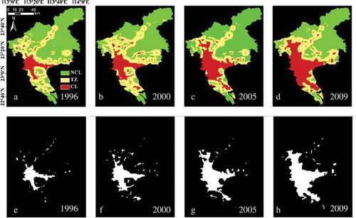
Four DMSP-OLS NSL images of Guangzhou in 1996, 2000, 2005, and 2009 are shown in )–. Based on the neighborhood statistics analysis tool of ArcGIS 9.3, we subtract the minimum-NSA-generated output raster from the maximum-NSA-generated output raster in a 3 × 3 cell neighborhood window. The subtracted results are generally referred to as a topographic map of NSL images. The results ()–) indicate that in the topographic map, the pixel values of the transition zones are significantly higher than those in HVR and LVR. An identical threshold value of 8 is found to be effective for distinguishing the transition zones from other parts of the topographic maps for all eight cities in 1996, 2000, 2005, and 2009. The results for Guangzhou are presented in )–(d) (yellow regions).
Figure 3. Deriving the topographic maps using the neighborhood statistics analysis method. Figure ‘a’–‘d’ shows the original DMSP/OLS imageries of the city of Guangzhou in 1996, 2000, 2005, and 2009, respectively; Figure ‘e’–‘h’ shows the corresponding topographic maps.
Figure 4. Extracting the built-up urban areas in HVR. Figure ‘a’–‘d’ represents the three classified areas (transition zones (TZ); built-up urban lands (BL); and non-built-up urban lands (NBL)) in 1996, 2000, 2005, and 2009, respectively; Figure ‘e’–‘h’ represents the extracted built-up areas in HVR.
3.2. Extracting the built-up urban areas in HVR
After the transition zones are identified, the entire regions are divided into three parts: the transition zones, built-up urban areas in HVR, and non-built-up areas in the LVR ()–). In general, the NSL values of HVR are always higher than those of a neighboring LVR. Therefore, the parts with NSL values that are relatively higher than the opposite side of the transition zone will be classified as built-up urban areas. In contrast, the parts with relatively lower NSL values will be classified as non-built-up lands. According to these relative differences in NSL values, the built-up urban areas in HVR are then distinguished from the non-built-up areas in LVR. The results are shown in )–.
3.3. Extracting the built-up urban areas in the transition zones
In this article, we separately generate two output raster data sets (MinOR5 and MinOR3) from the DMSP-OLS NSL images using the minimum NSA method in the 5 × 5 and 3 × 3 pixel windows. In the transition zones, the pixel values of MinOR5 in the built-up urban areas are usually smaller than those of MinOR3, while the pixel values of MinOR5 in non-built-up areas are usually equal to those of MinOR3 in the transition zones. Therefore, the built-up urban areas hidden in the transition zones can be identified by subtracting MinOR3 from MinOR5. The subtracted results are presented in )–(). An identical threshold value of −7 is effective for extracting the built-up urban areas hidden in the transition zones of all eight cities in 1996, 2000, 2005, and 2009. The built-up urban areas in the transition zones of Guangzhou are listed in )–.
Figure 5. Extracting the built-up urban areas hidden in the transition zones. Figure ‘a’–‘d’ represents subtracted results that are derived by subtracting the output raster of minimum-NSA in the 5 × 5 cell window from that in the 3 × 3 cell window in 1996, 2000, 2005, and 2009, respectively; Figure ‘e’–‘h’ represents the extracted built-up urban areas in the transition zones.
Note that 3 × 3 and 5 × 5 cell windows were used because a 3 × 3 cell window is the smallest window that allows the analysis of the neighborhood statistics and can thus ensure the highest accuracy for the extracted results. We compare the subtracted results between the minimum NSA methods operating in 4 × 4, 5 × 5, and 6 × 6 cell windows: the accuracies of the extracted built-up urban areas are 77.16%, 79.71%, and 75.95%, respectively, indicating that the 4 × 4 and 6 × 6 cell windows underestimate and overestimate approximately 3.19% and 4.72% of built-up urban areas, respectively. Thus, the combination of 5 × 5 and 3 × 3 cell windows is optimal for extracting built-up urban areas in transition zones.
3.4. Mapping the entire built-up urban area
Finally, the entire built-up urban area is obtained by overlaying the two regions ().
Figure 6. The entire built-up urban areas of Guangzhou extracted from NSL in 1996, 2000, 2005, and 2009.
4. Results and discussion
4.1. NSL-extracted built-up urban areas in the Pearl River Delta
The built-up urban areas in the eight cities from 1996 to 2009 ()–(t)) mapped using the proposed NSA method indicate that significant urban expansion occurred in the Pearl River Delta.
Figure 7. The built-up urban areas of eight cities in the Pearl River Delta of southern China in 1996, 2000, 2005, and 2009. Figure ‘a’–‘d’ represents the original DMSP/OLS NSL imageries; Figure ‘e’–‘h’ represents the Landsat TM/ETM+-extracted built-up urban areas; Figure ‘i’–‘l’ represents the NSL-extracted built-up urban areas using the global-fixed threshold method; Figure ‘m’–‘p’ represents the NSL-extracted built-up urban areas using the local-optimized threshold method; Figure ‘q’–‘t’ represents the NSL-extracted built-up urban areas using the proposed NSA method.
4.2. Validation of the total built-up urban area
Multi-temporal built-up urban areas extracted from the Landsat TM/ETM+ images during the same period ((e)–(h), Appendix 2) are selected to evaluate those ((q)–(t)) extracted from the DMSP-OLS NSL data ((a)–(d)) using the NSA method from 1996 to 2009. Because the spatial resolution of the DMSP-OLS images differs greatly from the Landsat TM/ETM+ data, we resample the Landsat TM/ETM+-extracted results to match the spatial resolution of the NSL data. The results reveal that the total pixel numbers of NSA-derived built-up urban areas of the eight cities are all consistent with those extracted from the Landsat TM/ETM+ data, with an average relative accuracy (RA) of 79.71% (R2 = 0.94, p < 0.001). Furthermore, the confusion matrix method in the Matlab software is used to assess the accuracies of the extracted built-up urban areas in the Pearl River Delta. The producer accuracy, user accuracy, and overall accuracy are 90.53, 83.55, and 82.07, respectively, on average ().
Table 2. Validation accuracies of DMSP/OLS NSL-extracted built-up urban areas using the confusion matrix method in Matab.
4.3. Comparison with the global-fixed and local-optimized threshold methods
The extracted results of the global-fixed and local-optimized threshold methods are presented in (i)–(l) and (m)–(p), respectively. Intuitive comparisons indicate that both the global-fixed and local-optimized threshold methods tend to overestimate the total area of built-up urban areas in cities with large urban extents due to the blooming effect of the DMSP-OLS data, as observed in Guangzhou, Dongguan, Foshan, Shenzhen, Zhongshan, and Zhuhai. In addition, the threshold methods tend to miss the small patches of built-up areas in the surrounding developing towns where the NSL is much lower. In contrast, our proposed NSA method not only accurately maps the large patches of built-up areas in urban regions but also successfully extracts small urban areas in the surrounding towns. The NSA method depends on the relative variations between neighboring built-up and non-built-up pixels (similar to the medium- or high-resolution methods), whereas the empirical threshold methods subjectively set identical thresholds for classification. Therefore, the proposed NSA method is more accurate and reliable than the global-fixed and local-optimized threshold methods when applied to cities with different urbanization levels.
4.4. Validation of the patch shapes of the built-up urban areas
The similarity of patch shapes is another vital factor for evaluating the accuracy of remotely sensed built-up urban areas. In addition to the total area index (CA), three other patch-shape indices (i.e., the landscape shape index (LSI), the contiguity index (CONTIG), and the perimeter area ratio (PARA)) were used to evaluate the similarities between the patch shapes of NSA-derived built-up urban areas and those from Landsat TM/ETM+ images (). The results are shown in and . Significantly positive correlations of patch shapes are observed between DMSP-OLS NSL- and Landsat TM/ETM+-derived built-up urban areas based on the CA (relative accuracy (RA) = 79.71%, R2 = 0.94, p < 0.001, )), LSI (R2 = 0.68, p < 0.001, )), CONTIG (R2 = 0.46, p < 0.001, )), and PARA (R2 = 0.63, p < 0.001, )). In summary, both the areas and patch shapes of NSA-extracted built-up urban areas are significantly consistent with those from the Landsat TM/ETM+ data.
Table 3. Definition of the landscape indices.
Table 4. Comparison of the landscape indices between DMSP/OLS NSL-mapped built-up urban areas with those from Landsat TM/ETM+ imageries.
Figure 8. Comparison of the landscape indices of DMSP/OLS NSA-derived built-up urban areas with those of Landsat TM/ETM+ images. (a) The total area (CA); (b) the landscape shape index (LSI); (c) the contiguity index (CONTIG); and (d) the perimeter area ratio (PARA).
4.5. Comparison with the statistical population data
The statistical built-up urban areas from the Statistical Yearbooks are generally smaller than the actual areas (Li and Yeh Citation2000; Yeh and Li Citation1997). Therefore, it is not feasible to use the statistical built-up urban areas for evaluating the remotely sensed results. Previous studies have demonstrated that statistical population data are highly correlated with built-up urban areas and can be effective in evaluating the mapping accuracies of remotely sensed built-up urban areas (Zhang and Seto Citation2011; Ma et al. Citation2012; Pandey, Joshi, and Setob Citation2013). In this article, the statistical population data of eight cities in 1996, 2000, 2005, and 2009 are used to indirectly assess the accuracies of our proposed method. The results show that the total NSL of NSA-extracted built-up urban lands is significantly correlated with the statistical urban populations (R2 = 0.62, p < 0.001) ().
Figure 9. Scatter diagrams between the total NSL of NSA-extracted built-up urban areas and statistical urban population.
4.6. Advantages and disadvantages of the NSA approach
Because of the large-scale coverage of the DMSP-OLS images, the NSL-based method is suitable for monitoring time series of urban expansions at regional, national, and global scales. Based on the relative variation between neighboring built-up and non-built-up pixels, the NSA method can accurately extract the large patches of built-up areas in urban regions as well as small urban areas in surrounding towns. However, the NSA method also has certain limitations, mainly due to its low spatial resolution. Compared with the medium- and high-resolution methods (Li et al. Citation2013; Qiu, Wu, and Miao Citation2014), the NSA method can only extract the built-up areas larger than 30 × 30 arc-second, which could of course emit stable lights at night.
5. Conclusions
A neighborhood statistics analysis (NSA) method was developed based on the relative spatial variations between neighboring built-up and non-built-up pixels of DMSP-OLS images. Multi-temporal case studies in eight cities of the Pearl River Delta indicated that the total areas of NSA-mapped results were highly correlated with those mapped from the Landsat TM/ETM+ data (R2 = 0.94; p < 0.001). Validations of patch shapes using landscape indices also revealed good correlations (R2 > 0.46; p < 0.001). In addition, the total NSL of the built-up urban areas of eight cities was significantly consistent with the statistical population data (R2 = 0.62; p < 0.001). It indirectly confirmed the effectiveness of our proposed NSA method (Zhang and Seto Citation2011; Ma et al. Citation2012; Pandey, Joshi, and Setob Citation2013).
The proposed NSA method, which significantly overcomes the disadvantages that are associated with the threshold-based methods, accurately maps both the large patches of built-up areas in urban regions and the small patches of built-up areas in surrounding towns. The proposed method is dependent on the relative variations in NSL values between neighboring built-up and non-built-up pixels rather than a pre-defined identical threshold.
Disclosure statement
No potential conflict of interest was reported by the authors.
Acknowledgments
We are grateful to four anonymous reviewers and the editor for their valuable comments, which have greatly improved the quality of this manuscript.
Additional information
Funding
References
- Angelelli, P., K. Nylund, O. H. Gilja, and H. Hauser. 2011. “Interactive Visual Analysis of Contrast-Enhanced Ultrasound Data Based on Small Neighborhood Statistics.” Computers & Graphics 35 (2): 218–226. doi:10.1016/j.cag.2010.12.005.
- Baugh, K., C. Elvidge, T. Ghosh, and D. Ziskin. 2010. “Development of a 2009 Stable Lights Product Using DMSP-OLS Data.” Proceedings of the 30th Asia-Pacific Advanced Network Meeting 30: 114–130.
- Berk, A., G. P. Anderson, P. K. Acharya, and E. P. Shettle. 2008. MODTRAN5.2.0.0 User’s Manual. Burlington, MA: Spectral Sciences.
- Bhatti, S. S., and N. K. Tripathia. 2014. “Built-Up Area Extraction Using Landsat 8 OLI Imagery.” GIScience and Remote Sensing 51 (4): 445–467. doi:10.1080/15481603.2014.939539.
- Bureau of Statistics of China. 2001. China City Statistical Yearbook – 2001. Beijing: China Statistics Press.
- Cao, X., J. Chen, H. Imura, and O. Higashi. 2009. “A SVM-Based Method to Extract Urban Areas from DMSP-OLS and SPOT VGT Data.” Remote Sensing of Environment 113: 2205–2209. doi:10.1016/j.rse.2009.06.001.
- Chen, X. Z., Y. X. Su, D. Li, G. Q. Huang, W. Q. Chen, and S. S. Chen. 2012. “Study on the Cooling Effects of Urban Parks on Surrounding Environments Using Landsat TM Data: A Case Study in Guangzhou, Southern China.” International Journal of Remote Sensing 33 (18): 5889–5914. doi:10.1080/01431161.2012.676743.
- Croft, T. A. 1978. “Nighttime Images of the Earth from Space.” Scientific American 239 (1): 86–98. doi:10.1038/scientificamerican0778-86.
- Elvidge, C. D., K. E. Baugh, J. B. Dietz, T. Bland, P. C. Sutton, and H. W. Kroehl. 1999. “Radiance Calibration of DMSP-OLS Low-Light Imaging Data of Human Settlements.” Remote Sensing of Environment 68: 77–88. doi:10.1016/S0034-4257(98)00098-4.
- Elvidge, C. D., K. E. Baugh, V. H. Hobson, E. A. Kihn, H. W. Kroehl, E. R. Davis, and D. Cocero. 1997. “Satellite Inventory of Human Settlements Using Nocturnal Radiation Emissions: A Contribution for the Global Toolchest.” Global Change Biology 3: 387–395. doi:10.1046/j.1365-2486.1997.00115.x.
- Elvidge, C. D., M. L. Imhoff, K. E. Baugh, V. R. Hobson, I. Nelson, J. Safran, J. B. Dietz, and B. T. Tuttle. 2001. “Night-Time Lights of the World: 1994–1995.” ISPRS Journal of Photogrammetry and Remote Sensing 56: 81–99. doi:10.1016/S0924-2716(01)00040-5.
- Elvidge, C. D., B. T. Tuttle, P. C. Sutton, K. E. Baugh, A. T. Howard, C. Milesi, B. Bhaduri, and R. Nemani. 2007. “Global Distribution and Density of Constructed Impervious Surfaces.” Sensors 7: 1962–1979. doi:10.3390/s7091962.
- Elvidge, C. D., D. Ziskin, K. Baugh, B. T. Tuttle, T. Ghosh, D. W. Pack, E. H. Erwin, and M. Zhizhin. 2009. “A Fifteen Year Record of Global Natural Gas Flaring Derived from Satellite Data.” Energies 2 (3): 595–622. doi:10.3390/en20300595.
- Fang, C. 2009. “Urbanization and Urban Development in China after the Reform and Opening-Up.” [In Chinese.] Economic Geography 29 (1): 19–25.
- He, C., P. Shi, J. Li, J. Chen, Y. Pan, J. Li, L. Zhuo, and T. Ichinose. 2006. “Restoring Urbanization Process in China in the 1990s by Using Non-Radiance-Calibrated DMSP/OLS Nighttime Light Imagery and Statistical Data.” Chinese SCI Bull 51 (13): 1614–1620. doi:10.1007/s11434-006-2006-3.
- Henderson, M., E. T. Yeh, P. Gong, C. D. Elvidge, and K. E. Baugh. 2003. “Validation of Urban Boundaries Derived from Global Night-Time Satellite Imagery.” International Journal of Remote Sensing 24 (3): 595–609. doi:10.1080/01431160304982.
- Imhoff, M. L., L. Bounoua, R. DeFries, W. T. Lawrence, D. Stutzer, C. J. Tucker, and T. Ricketts. 2004. “The Consequences of Urban Land Transformation on Net Primary Productivity in the United States.” Remote Sensing of Environment 89: 434–443. doi:10.1016/j.rse.2003.10.015.
- Imhoff, M. L., W. T. Lawrence, C. Elvidge, T. Paul, E. Levine, and M. Prevalsky. 1997a. “Using Nighttime DMSP/OLS Images of City Lights to Estimate the Impact of Urban Land Use on Soil Resources in the United States.” Remote Sensing of Environment 59: 105–117. doi:10.1016/S0034-4257(96)00110-1.
- Imhoff, M. L., W. T. Lawrence, D. C. Stutzer, and C. D. Elvidge. 1997b. “A Technique for Using Composite DMSP/OLS ‘City Lights’ Satellite Data to Map Urban Area.” Remote Sensing of Environment 61: 361–370. doi:10.1016/S0034-4257(97)00046-1.
- Kramer, H. J., ed. 1994. “DMSP (Defense Meteorological Satellite Program) and DMSP Data Availability: Visible and Infrared Images.” In Observation of the Earth and Its Environment: Survey of Missions and Sensors, 61–67. Berlin: Springer Verlag.
- Lawrence, W. T., M. L. Imhoff, N. Kerle,and, and D. Stutzer. 2002. “Quantifying Urban Land Use and Impact on Soils in Egypt Using Diurnal Satellite Imagery of the Earth Surface.” International Journal of Remote Sensing 23: 3921–3937. doi:10.1080/01431160110115951.
- Li, G. Y., D. S. Lu, E. Moran, and S. Hetrick. 2013. “Mapping Impervious Surface Area in the Brazilian Amazon Using Landsat Imagery.” GIScience and Remote Sensing 50: 172–183. doi:10.1080/15481603.2013.780452.
- Li, X., and A. G. O. Yeh. 2000. “Modelling Sustainable Urban Development by the Integration of Constrained Cellular Automata and GIS.” International Journal of Geographical Information Science 14 (2): 131–152. doi:10.1080/136588100240886.
- Liu, J., M. Liu, H. Tian, D. Zhuang, Z. Zhang, W. Zhang, X. Tang, and X. Deng. 2005. “Spatial and Temporal Patterns of China’s Cropland during 1990–2000: An Analysis Based on Landsat TM Data.” Remote Sensing of Environment 98: 442–456. doi:10.1016/j.rse.2005.08.012.
- Liu, J., M. Liu, D. Zhuang, Z. Zhang, and X. Deng. 2003. “Study on Spatial Pattern of Land-Use Change in China during 1995–2000.” Science in China Series D 46 (4): 373–384. doi:10.1360/03yd9033.
- Liu, J., Z. Zhang, X. Xu, W. Kuang, W. Zhou, S. Zhang, R. Li, et al. 2010. “Spatial Patterns and Driving Forces of Land Use Change in China during the Early 21st Century.” Journal of Geographical Sciences 20 (4): 483–494. doi:10.1007/s11442-010-0483-4.
- Liu, Z. F., C. Y. He, Q. F. Zhang, Q. X. Huang, and Y. Yang. 2012. “Extracting the Dynamics of Urban Expansion in China Using DMSP-OLS Nighttime Light Data from 1992 to 2008.” Landscape and Urban Planning 106: 62–72. doi:10.1016/j.landurbplan.2012.02.013.
- Lo, C. P. 2001. “Modeling the Population of China Using DMSP Operational Linescan System Nighttime Data.” Photogranimetric Engineering & Remote Sensing 67 (9): 1037–1047.
- Lu, D. S., H. Q. Tian, G. M. Zhou, and H. L. Ge. 2008. “Regional Mapping of Human Settlements in Southeastern China with Multisensor Remotely Sensed Data.” Remote Sensing of Environment 112: 3668–3679. doi:10.1016/j.rse.2008.05.009.
- Ma, T., C. Zhou, T. Pei, S. Haynie, and J. Fan. 2012. “Quantitative Estimation of Urbanization Dynamics Using Time Series of DMSP/OLS Nighttime Light Data: A Comparative Case Study from China’s Cities.” Remote Sensing of Environment 124: 99–107. doi:10.1016/j.rse.2012.04.018.
- Mcfeeters, S. K. 1996. “The Use of the Normalized Difference Water Index (NDWI) in the Delineation of Open Water Features.” International Journal of Remote Sensing 17 (7): 1425–1432. doi:10.1080/01431169608948714.
- Milesi, C., C. D. Elvidge, R. R. Nemani, and S. W. Running. 2003. “Assessing the Impact of Urban Land Development on Net Primary Productivity in the Southeastern United States.” Remote Sensing of Environment 86: 401–410. doi:10.1016/S0034-4257(03)00081-6.
- Ottinger, M., C. Kuenzer, G. H. Liu, S. Q. Wang, and S. Dech. 2013. “Monitoring Land Cover Dynamics in the Yellow River Delta from 1995 to 2010 Based on Landsat 5 TM.” Applied Geography 44: 53–68. doi:10.1016/j.apgeog.2013.07.003.
- Owen, T. W. 1998. “Using DMSP-OLS Light Frequency Data to Categorize Urban Environments Associated with US Climate Observing Stations.” International Journal of Remote Sensing 19: 3451–3456. doi:10.1080/014311698214127.
- Pandey, B., P. K. Joshi, and K. C. Setob. 2013. “Monitoring Urbanization Dynamics in India Using DMSP/OLS Night Time Lights and SPOT-VGT Data.” International Journal of Applied Earth Observation and Geoinformation 23: 49–61. doi:10.1016/j.jag.2012.11.005.
- Qi, Q. M., and M. Chopping. 2007. “Expansion of Urban Area in the Yellow River Zone, Inner Mongolia Autonomous Region, China, from DMSP OLS Nighttime Lights Data.” Geoscience and Remote Sensing Symposium, Barcelona, July 23–28, 2002–2005.
- Qiu, X. M., S.-S. Wu, and X. Miao. 2014. “Incorporating Road and Parcel Data for Object-Based Classification of Detailed Urban Land Covers from NAIP Images.” GIScience and Remote Sensing 51: 498–520. doi:10.1080/15481603.2014.963982.
- Richter, R. 2011. Atmospheric/Topographic Correction for Satellite Imagery ATCOR-2/3 User Guide. DLR IB 565-01/11. Wessling: DLR Report-German Atmosphere Center.
- Schneider, A., M. A. Friedl, D. K. McIver, and C. E. Woodcock. 2003. “Mapping Urban Areas by Fusing Multiple Sources of Coarse Resolution Remotely Sensed Data.” Photogrammetric Engineering and Remote Sensing 69: 1377–1386. doi:10.14358/PERS.69.12.1377.
- Shi, K. F., C. Huang, B. L. Yu, B. Yin, Y. X. Huang, and J. P. Wu. 2014. “Evaluation of NPP-VIIRS Night-Time Light Composite Data for Extracting Built-Up Urban Areas.” Remote Sensing Letters 5 (4): 358–366. doi:10.1080/2150704X.2014.905728.
- Small, C., F. Pozzi, and C. D. Elvidge. 2005. “Spatial Analysis of Global Urban Extent from DMSP-OLS Night Lights.” Remote Sensing of Environment 96: 277–291. doi:10.1016/j.rse.2005.02.002.
- Su, Y. X., X. Z. Chen, Y. Li, J. S. Liao, Y. Y. Ye, H. O. Zhang, N. S. Huang, and Y. Q. Kuang. 2014. “China’s 19-Year City-Level Carbon Emissions of Energy Consumptions, Driving Forces and Regionalized Mitigation Guidelines.” Renewable and Sustainable Energy Reviews 35: 231–243. doi:10.1016/j.rser.2014.04.015.
- Su, Y. X., G. Q. Huang, X. Z. Chen, and S. S. Chen. 2010. “The Cooling Effect of Guangzhou City Parks to Surrounding Environments.” [In Chinese.] Acta Ecologica Sinica 30 (18): 4905–4918.
- Sutton, P., D. Roberts, C. Elvidge, and K. Baugh. 2001. “Census from Heaven: An Estimate of the Global Human Population Using Night-Time Satellite Imagery.” International Journal of Remote Sensing 22 (16): 3061–3076. doi:10.1080/01431160010007015.
- Sutton, P. C., T. J. Cova, and C. D. Elvidge. 2006. “Mapping ‘Exurbia’ in the Conterminous United States Using Nighttime Satellite Imagery.” Geocarto International 21 (2): 39–45. doi:10.1080/10106040608542382.
- Sutton, P. C., S. J. Anderson, C. D. Elvidge, B. T. Tuttle, and T. Ghosh. 2009. “Paving the Planet: Impervious Surface as Proxy Measure of the Human Ecological Footprint.” Progress in Physical Geography 33: 510–527. doi:10.1177/0309133309346649.
- Wei, Y., H. Liu, W. Song, B. Yu, and C. Xiu. 2014. “Normalization of Time Series DMSP-OLS Nighttime Light Images for Urban Growth Analysis with Pseudo Invariant Features.” Landscape and Urban Planning 128: 1–13. doi:10.1016/j.landurbplan.2014.04.015.
- Yeh, T. W., and H. N. Li. 1997. “Factorization Theorems, Effective Field Theory, and Nonleptonic Heavy Meson Decays.” Physical Review D 56 (3): 1615. doi:10.1103/PhysRevD.56.1615.
- Yu, B. L., S. Shu, H. X. Liu, W. Song, J. P. Wu, L. Wang, and Z. Q. Chen. 2014. “Object-Based Spatial Cluster Analysis of Urban Landscape Pattern Using Nighttime Light Satellite Images: A Case Study of China.” International Journal of Geographical Information Science 28 (11): 2328–2355. doi:10.1080/13658816.2014.922186.
- Zha, Y., S. Y. Ni, and S. Yang. 2003. “An Effective Approach to Automatically Extract Urban Land-Use from TM Imagery.” [In Chinese.] Journal of Remote Sensing 7 (1): 37–40.
- Zhang, Q., and K. C. Seto. 2011. “Mapping Urbanization Dynamics at Regional and Global Scales Using Multi-Temporal DMSP/OLS Nighttime Light Data.” Remote Sensing of Environment 115: 2320–2329. doi:10.1016/j.rse.2011.04.032.
- Zhang, Q. F., C. Y. He, and Z. F. Liu. 2014. “Studying Urban Development and Change in the Contiguous United States Using Two Scaled Measures Derived from Nighttime Lights Data and Population Census.” GIScience and Remote Sensing 51: 63–82. doi:10.1080/15481603.2014.883212.
- Zhou, Y., S. J. Smith, C. D. Elvidge, K. Zhao, A. Thomson, and M. Imhoff. 2014. “A Cluster-Based Method to Map Urban Area from DMSP/OLS Nightlights.” Remote Sensing of Environment 147: 173–185. doi:10.1016/j.rse.2014.03.004.
Appendix 1. Neighborhood statistics analysis (NSA) method
The neighborhood statistics function is a focal function that computes an output raster in which the value at each location is a function of the input cells in a specified neighborhood window (such as the 3 × 3 cell window) of the location. For each cell in the input raster, the neighborhood statistics function computes a statistic based on the value of the processing cell and the value of the cells within the specified neighborhood window; this value is set as the value of the corresponding cell location on the output raster. For example, each pixel value of the output raster using the maximum (or minimum) NSA method is the maximum (or minimum) pixel value of the specified neighborhood cell window. To illustrate the maximum (or minimum) neighborhood statistics processing, we separately present the single input raster cell and the entire raster data set in the diagram of . For the 3 × 3 cell window, the maximum (or minimum) value of neighboring cells for the processing cell (highlighted in gray) equals to 6 (or 1). Thus, a value of 6 (or 1) is given to the cell in the output raster that is in the same location as the processing cell in the input raster. As for the entire raster data set, each cell in the output raster is calculated by searching the minimum values in a 3 × 3 cell neighborhood window for each cell. If a cell of NoData is present in the neighborhood, then it will be ignored in the processing.
Figure A1. Maximum/minimum neighborhood statistics analysis for single cells and for the entire data set.
Appendix 2. Extracting built-up urban areas from Landsat TM/ETM+ images
Because of the fine spatial resolution of Landsat TM/ETM+ data (30 × 30 m2), built-up urban areas extracted from the Landsat TM/ETM+ images are feasible and acceptable for evaluating the mapping results of NSL data (Cao et al. Citation2009; He et al. Citation2006; Henderson et al. Citation2003; Small, Pozzi, and Elvidge Citation2005; Sutton, Cova, and Elvidge 2006). In this article, a decision-tree method was developed to extract the built-up urban areas from Landsat TM/ETM+ images based on the commonly used spectral-analysis algorithms. The technical approach is shown in .
Figure A2. Technical approach for extracting built-up urban areas from Landsat TM/ETM+ images.
First, we conducted a pre-processing geometric and atmospheric correction on the Landsat TM/ETM+ images. For the geometric corrections, a total of 11 control points were collected at the junctions of major rivers and roads, with a RMSE of less than 0.25 pixels. For the atmospheric corrections, we used the Atmospheric and Topographic Correction (ATCOR2) software package (Richter Citation2011) to calculate sensor-specific atmospheric look-up tables (LUT) based on the Moderate Resolution Atmospheric Transmission Model (MODTRAN5) codes (Berk et al. Citation2008).
Three spectral indices (normalized difference vegetation index, NDVI; normalized difference water index, NDWI (Mcfeeters Citation1996); and normalized difference built-area index, NDBI (Zha, Ni, and Yang Citation2003)) were used to distinguish vegetated lands, wetlands, and bare grounds from built-up urban areas. The definitions of NDVI, NDWI, and NDBI are as follows: NDVI = (TM4-TM3)/(TM4+TM3), NDWI = (TM2-TM4)/(TM2+TM4), and NDBI = (TM5-TM4)/(TM5+TM4). The NDVI of vegetated regions is always larger than zero and is thus feasible for extracting vegetated lands from other lands. Similarly, the DN values of TM2 in wetlands are obviously higher than those of TM4, so wetlands were also excluded using the NDWI (NDWI > 0). The remaining regions contained only two land cover types: built-up urban areas and bare ground. The locations where NDBI > 0 were distinguished as built-up urban areas (Zha, Ni, and Yang Citation2003).This article used higher spatial resolution SPOT remote sensing images to validate the classification results from Landsat TM data in 2005 and 2009. For each year, 100 samples were selected to validate the extraction results of built-up urban areas. The proportion of matched pixels was 81.29% in 2005 and 82.02% in 2009. Because there were no sufficient field data available to assess the classification accuracy in 1996 and 2000, the Landsat TM scenes were the only reliable reference data for the classification validations. Therefore, we compared the classification results with the original Landsat TM images using Ottinger’s method (Ottinger et al. Citation2013). The accuracies in 1996 and 2000 were 85.02 and 79.64%, respectively.