Comparison of DEMS derived from USGS DLG, SRTM, a statewide photogrammetry program, ASTER GDEM and LiDAR: implications for change detection

Abstract

Many digital elevation models (DEMs) now exist, enabling quantitative assessments of topographic change through DEM subtraction. However, many of these DEMs are inherently different – their source data, preprocessing, and interpolation procedures introduce varying amounts of error, which are partially correlated with the local topographic situation (e.g. slope, aspect, and elevation of any given location). Understanding of these differences and potential errors is necessary prior to change detection analysis in order to incorporate the inherent uncertainties into the analysis of topographic change. This study evaluated available DEMs in the Mud 7.5′ United States Geological Survey (USGS) topographic quadrangle in West Virginia, USA. We compare DEMs derived from the USGS digital line graphs (DLGs), the Shuttle Radar Topography Mission (SRTM), a statewide photogrammetric DEM, and the Advanced Spaceborne Thermal Emission and Reflection (ASTER) Global DEM v2, to a LiDAR DEM. Using the LiDAR data as a reference (RMSE 0.12 m), the USGS DLG and the SAMB showed low RMSE, while the SRTM and GDEM exhibited high RMSE and a systematic negative bias.

Keywords:

• DEM
• topographic change
• DEM of difference
• DEM error

Introduction

A growing field of geomorphologic analyses relies on topographic change calculated from digital elevation model (DEM) differencing (Khalsa et al. 2004; Martínez-Casasnovas, Ramos, and Poesen 2004; Huggel et al. 2008; Wheaton et al. 2009; Blanchard, Rogan, and Woodcock 2010; Hicks 2012; James et al. 2012; Ren et al. 2014). As anthropogenic modification of the earth’s surface continues to drastically change the landscape and environment (Hooke 1999, 2000; Phillips 2004; Gesch 2005, 2014), there is an increasing demand for analyses involving topographic change detection. Though the technology exists to create and utilize high-resolution, high-accuracy elevation data for the precise quantification of topographic change, such data is temporally limited and often expensive to acquire. Furthermore, globally and regionally collected DEMs extend back to 2000 and are widely available to a variety of users. However, such DEMs differ greatly in terms of their collection procedures, resolution, and accuracy levels (Bolstad and Stowe 1994; Gong et al. 2000). Thus, studies of topographic change detection are confronted with two potential sources of error: (1) comparison of DEMs that reflect different surfaces, meaning that the elevation values used to create each DEM may not necessarily model the same ‘ground’ surface; and (2) the traditional conceptualization of DEM error, that includes horizontal locational error (with both x and y components), and vertical measurement error. It is important to understand that these DEM-specific uncertainties should be accommodated in change detection analysis, however, very little literature exists to guide such efforts. It is the objective of this paper to elucidate the differences between commonly available DEMs, to evaluate how these inconsistencies translate to differing accuracies between the DEMs, and to interpret the impact of these observed inaccuracies on a hypothetical topographic change detection.

Grid-based DEMs are created through the interpolation of point- or line-based elevation values which may be collected through in situ sampling, photogrammetry, or active remote sensors. Each data collection method has varying interaction with surface objects (most importantly vegetation), and thus incorporates varying levels of ‘error’ in the resultant DEM. Interpolation methods can also introduce substantial error to a DEM (Aguilar et al. 2005; Chaplot et al. 2006; Chu et al. 2014). These differences complicate direct comparison of one DEM with another DEM in change detection analysis and must be understood, and preferably quantified, prior to topographic change quantification. This paper compares the accuracy of several widely available DEMs, including two global DEMs, a national-scale DEM, and a state-wide DEM to LiDAR elevation data for a study area in southern West Virginia (WV). Though other studies have focused on quantifying the individual accuracy of each DEM examined here, this study is the first to our knowledge to simultaneously compare the Advanced Spaceborne Thermal Emission and Reflection (ASTER) Global DEM (GDEM), the Shuttle Radar Topography Mission (SRTM), United States Geological Survey (USGS) 7.5′ topographic digital line graphs (DLGs), and a state-wide photogrammetric DEM for a single area of interest.

In recent years, technological advances have improved the frequency of DEM creation and update, as well as the spatial resolution of the released models. However, the spatial extent of new elevation mapping campaigns is highly variable and many new DEMs are collected for small spatial extents, such as individual cities or counties. While these new DEMs are valuable improvements in data availability for their specific area of coverage, they do not match the resolution and accuracy of the ‘best available’ regional-scale DEMs to which they might be compared in topographic change studies.

Background

In order to clarify potential sources of elevation error and inaccuracy, the following section reviews the data collection and preprocessing methods for each of the DEMs assessed in this study. This section focuses particularly on what we have termed the “conceptual error”, namely the differences in the nature of the surface sensed by the remote-sensing technology used.

USGS DLG

One of the most widely available elevation datasets in the United States is produced by the USGS in the form of 1:24,000 scale contour-based topographic maps (also referred to as 7.5′ topographic quadrangle maps). Prior to computer-automated collection methods, contour maps were scribed manually from aerial imagery using stereoplotters. With the advent of computer automation, photogrammetric software is now used to generate a set of mass points, break lines, and special points, from which elevation contours are automatically interpolated (Molander 2001; Hodgson et al. 2003). Break lines are inserted to modify the interpolated values where the topography changes abruptly, such as ridgelines or stream valleys. USGS 7.5′ topographic maps were published as they were completed for each quadrangle, beginning in the 1940s and were officially completed in 1991 (Evans and Frye 2009; USGS 2013). In recent years, only minor revisions have been made to individual quadrangles, and the series has been converted to a digital format (USGS 2013). Since the map for each quadrangle was published and is updated individually, neighboring quadrangles frequently have different publication years (USGS 2013). This becomes problematic in topographically dynamic areas, because the contours of one quadrangle may differ substantially from those of the adjoining quadrangle.

USGS topographic map accuracy standards are based on the testing of points within the map space, and are worded to account for contour-based elevation models (USGS 2006). In 7.5′ quadrangle maps with a 20-ft contour interval, the accuracy standard translates roughly to a horizontal error of <12.1 m and a vertical error of <3.05 m.

Conversion of the published topographic contours to digital format was performed through high-resolution scanning of the printed maps or through manual digitization. Although each of these procedures potentially introduces error in the data, the amount of error introduced by digitization is generally negligible. Although the DLGs produced by the USGS do not carry quantified accuracy statements, they have been found to maintain accuracy similar to that of the original maps (USGS 1993).

From their digitized polyline format, contours must be interpolated to a grid by the user. This interpolation introduces error in the accuracy of the generated grid-based elevation surface. Interpolation of contours, particularly in areas of low relief, may poorly represent the true variation of the ground surface. Conversely, areas of high relief are shown by closely drawn contours, which may become less accurate in digitized format (Hengl and Evans 2009). Furthermore, a multitude of interpolation algorithms optimized for different topographic situations exist. The most accurate and commonly used of these ensures correct hydrologic drainage of the modeled topographic surface (Hutchinson 1988, 1989, 2006).

Unlike the National Elevation Dataset (NED), a conglomeration of ‘best available’ elevation datasets produced by the USGS through the National Map, DLGs are useful in change detection because they come from a single, specific data source and carry with them a specific publication date – two key factors in topographic change analysis. When using the DLGs in the quantification of elevation change, it is important to remember that the source data is modified four times from the original photogrammetrically measured elevation values: once when the contours are drawn (which smoothes and generalizes topography across the earth’s surface), once when 1:24,000 topographic contour maps are digitized (data modification in this step is generally regarded as minor), once when the digitized contour lines are interpolated to a grid (where original data values are potentially lost in favor of a grid-based surface model), and finally when the DEM values are modified to incorporate correct hydrologic drainage.

SRTM

The SRTM collected a global elevation dataset using C-band and X-band interferometric synthetic aperture radar (IFSAR) over 11 days in 2000 (Hensley, Munjy, and Rosen 2007). Though data for the two bands were collected simultaneously, the coverage of the X-band is geographically limited compared to that of the C-band, and the DEM processing of the two datasets was carried out separately by the German Aerospace Center (DLR) and the National Aeronautics and Space Administration (NASA) Jet Propulsion Laboratory (JPL), respectively. Some studies have found the X-band DEM to contain more outliers than the C-band DEM, as well as a systematic bias of higher error (around 10 m) in certain regions of the globe (Hoffmann and Walter 2006).

In general, IFSAR remote sensing has several advantages over photogrammetric elevation collection, such as cloud penetration, potential nighttime data collection, partial vegetation penetration, control over the angle of illumination, and the flexibility of different polarizations (Jensen 2007). Additionally, the SRTM 30° to 58° off-nadir swaths were collected from an altitude of 233 km, yielding a wide swath width of 225 km (USGS 2009), and allowing for global coverage in only 11 days.

The DEM produced from SRTM data has a spatial resolution of 1″ (1 arc second or approximately 30 m), which was degraded to 3″ outside the United States until 2014, and a vertical accuracy performance goal of ±16 m (Pierce et al. 2006). Evaluations of its vertical accuracy found the SRTM to have an average absolute height error of 9 m in North America (Rodriguez, Morris, and Belz 2006), however in the mountainous, heavily forested region of Appalachia, the average error was found to be higher (Bolstad and Stowe 1994; Blanchard, Rogan, and Woodcock 2010). In WV, Massachusetts, and New Hampshire, the SRTM represented a surface well above the ground, but not consistently at the canopy level (Hofton et al. 2006; Passini, Jacobsen, and Passini 2007). The varying roughness of the vegetation canopy contributes to this inconsistent surface detection (Hodgson et al. 2003; Hensley, Munjy, and Rosen 2007). In mountainous regions, IFSAR returns may also be affected by foreshortening, layover, and shadow, resulting in higher errors (Guth 2006; Gómez et al. 2012). These factors should be considered and incorporated as inaccuracies in elevation change detections.

ASTER GDEM

The ASTER sensor located on board the Terra satellite, has nadir- and aft-looking near infrared (NIR) cameras which produce a stereopair for every scene collected. The ASTER Global DEM (GDEM) version 1 (v1) was created photogrammetrically from a compilation of cloud-free ASTER stereopairs. Published in 2009, with a 30 m horizontal posting and a 20 m (95% confidence) stated accuracy, it was validated globally by NASA at 25 m root mean squared error (RMSE) (Chirico, Malpeli, and Trimble 2012), and has been independently validated in North America at an RMSE of 10.45 m (Abrams et al. 2010). A metadata raster accompanying the elevation raster indicates the number of ASTER scenes used in the calculation of each pixel’s elevation. Two key sources of error exist in the GDEM v1: residual cloud artifacts and flaws in the stacking algorithm (Chirico, Malpeli, and Trimble 2012; Hirano, Welch, and Lang 2003). Additionally, an overall negative bias has been identified in multiple studies (Slater et al. 2011; Hirt, Filmer, and Featherstone 2010; Chirico, Malpeli, and Trimble 2012). A second version of the ASTER GDEM (v2, released by NASA in 2011) includes additional scene coverage, a smaller correlation kernel, and improved water masking, and achieves a reported accuracy of 17 m (ASTER GDEM Validation Team 2011). The GDEM v2 has been independently tested to have an RMSE of 8.6 m (Gesch et al. 2012).

While the inclusion of multiple imagery dates in the computation of each pixel’s elevation value improves the extent of cloud-free imagery (thereby extending the range of the DEM), it potentially limits the use of the GDEM for change detection studies. In topographically dynamic areas, the multiple image dates introduce inconsistency to the change detection and result in a highly variable amount of elevation change over short distances.

Statewide Addressing and Mapping Board DEM

The WV Statewide Addressing and Mapping Board (SAMB) was established in 2001 through legislation that aimed to provide rural areas of the state with city-type addressing to improve the infrastructure, utilities, emergency management, and homeland security of the state (WVDHSEM 2014). To facilitate this mapping, 2 ft true color aerial imagery was flown for the entire state in the spring of 2003 and the spring of 2004. Break lines and elevation mass points at 3 m intervals were extracted photogrammetrically from the aerial photos at a vertical accuracy of ± 10 ft by a privately contracted geospatial firm. The resultant digital terrain model (DTM) was interpolated to a 3 m DEM by the WV GIS Technical Center (WVGISTC), in cooperation with the USGS. The final bare-earth DEM product has a tested vertical accuracy of 0.209 m (Fedorko 2005).

LiDAR

Topographic LiDAR is a relatively recent source of elevation data that relies upon precisely timed measurements of a laser from a position in space calculated from a global positioning system (GPS) device and an inertial measurement unit (IMU). Distance from the laser to the ground is calculated from the return time of the NIR laser beam. This distance value is converted to a ground elevation using the GPS/IMU measurements of the sensor’s position in space (Hodgson et al. 2003; Fowler 2007). The accuracy of LiDAR elevation data depends on the accurate measurement of the position and orientation of the sensor, and is also affected by the sensor’s field of view, scan rate, and acquisition altitude. Vertical errors are generally less than 0.3 m (Daniel and Tennant 2007). When the LiDAR pulse encounters vegetation, the radiation is scattered by the leaf’s intercellular surfaces, both back toward the sensor and also forward on its original path. Although every beam may not reach the ground in areas of dense vegetation, generally, the high sampling density of LiDAR sensors overcomes vegetation coverage and yields elevation values representative of the ground surface (Rosette et al. 2012; Fowler 2007).

DiCicco (2011) performed an accuracy assessment of the LiDAR dataset used in this study by ground-surveying 321 points divided among four land cover categories across the southern WV coalfields area of interest. The accuracy assessment reported a consolidated RMSE of 0.118 m for the LiDAR dataset.

Summary

The goal of this background section is to call attention to the conceptual differences between different DEMs by briefly reviewing their data collection methods and processing. Table 1 summarizes each of the DEMs used in this this study in terms of creation date, method, target, and tested accuracies.

Table 1. DEM datasets evaluated in this study.

Dataset	Date	Native cell size	Creation method	Target accuracy	Estimated accuracy	Season of collection
DLGDEM	1976	30 m	Aerial photogrammetry	<3.09 m	<3.05 m^a	Leaf-off
SRTMDEM	2000	30 m	C-band IFSAR	16 m	9 m^b	February
SAMBDEM	2003	3 m	Aerial photogrammetry	±10 ft	2.091 m^c	April
GDEM	2009	30 m	Satellite photogrammetry	25 m	10.45 m^d	Multiple
LiDARDEM	2010	3 m	LiDAR	<0.3 m	0.209 m^e	Leaf-off

Notes: ^aUSGS (2006).

^bRodríguez, Morris, and Belz (2006); Bolstad and Stowe (1994); Blanchard, Rogan, and Woodcock (2010); Hofton et al. (2006); Passini, Jacobsen, and Passini (2007).

^cFedorko (2005).

^dAbrams et al. (2010).

^eDiCicco (2011).

It should be clear that a DEM created from topographic map contours is inherently different from a DEM created from IFSAR or LiDAR data. The rest of this study compares each of the above-mentioned types of DEMs to a reference DEM for a mountainous study site in southern WV, USA.

Study area

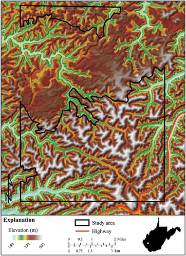
The study site is located within the Mud 7.5′ topographic quadrangle in southern WV (Figure 1), and is used as a case study to evaluate available DEMs for change detection applications. This study area, which includes parts of Lincoln, Boone, and Logan counties, is in a heavily forested section of the Appalachian Mountains. Over the past several decades, the northern part of the Mud quadrangle has experienced extensive topographic change due to surface mining activity in the Hobet Mine Complex. This mined area is excluded from the analysis. The southern part of the quadrangle is currently unaffected by mining, and thus is isolated for this comparison of DEM accuracies.

Figure 1. Location of the study area within the 7.5′ topographic quadrangle. For full color versions of the figures in this paper, please see the online version.

Data and preprocessing

Elevation data used in this study include the USGS DLG, the SRTM, the ASTER GDEM v1, the SAMB, and LiDAR data (see Table 1). The most recent (and presumably most accurate) elevation dataset available for the Mud Quadrangle is a LiDAR-based DEM collected in 2010. Since the tested accuracy of the LiDAR (RMSE 0.209 m) is substantially lower than the expected error in the other datasets, the LiDAR DEM (referred to hereafter as ‘LiDARDEM’) is used as the reference topographic surface to which all other DEMs are compared to estimate their error.

All DEM datasets were obtained at a 3 × 3 topographic quadrangle extent surrounding the study area. This extent allowed for a one-quadrangle ‘buffer’ between the study area and the data’s edge, preventing potential edge-artifacts. The nine 7.5′ Topographic Quadrangle DLGs were downloaded from the USGS EarthExplorer portal, as were the SRTM void-filled dataset, and the ASTER L1B GDEM dataset. The SAMBDEM was downloaded from the WVGISTC at <http://wvgis.wvu.edu>, and the LiDAR DEM was downloaded from WV View at <http://www.wvview.org>.

Datasets were downloaded in the Universal Transverse Mercator projection of the North American Datum 1983 for zone 17 North (UTM NAD83 Z17N) or were transformed to this projection using cubic convolution, then converted to a grid and mosaicked as necessary. All DEMs were initially downloaded in their native resolution, then resampled to a consistent 30 m grid by cubic convolution (following the mosaicking procedure). The resultant 30 m DEMs were clipped to a 1 km buffer around the Mud quadrangle.

Other datasets used in this study include a boundary shapefile encompassing surface mining that was manually interpreted and digitized from 2011 National Agricultural Imaging Program (NAIP) imagery. This boundary was used to mask areas disturbed by mining from the DEM comparison. The Multi-Resolution Land Characteristics Consortium (MRLC) National Land Cover Dataset (NLCD) 2006 was also downloaded for the study area and reclassified to generalize the land cover into the following classes: developed, forested, shrubland/ cropland, and grassland/pasture. Areas of the quadrangle disturbed by mining were masked from the reclassified NLCD dataset, and the remaining areas and boundaries of each of the six land cover classes were used to create a 1000 point stratified (by proportional area) random sample, with a minimum point separation distance of 86 m.

Methods

Each DEM was first spatially aligned with the LiDARDEM to minimize the horizontal locational error introduced through spatial misregistration of the two raster grids. A horizontal registration procedure, based on optimization standard deviation of differences, was performed for each DEM individually in Erdas Imagine. The optimal shift results were used to spatially register the DEM to the LiDARDEM. This spatial realignment effectively minimizes the horizontal locational error between the datasets, allowing us to focus on the elevation differences between the datasets, which arise due to due to differences in the nature of the surfaces sensed (i.e. conceptual error) and the measurement uncertainty.

Next, following the deterministic error surface methods of Gonga-Saholiariliva et al. (2011), a difference raster was generated for each DEM by subtracting it from the LiDARDEM (LiDARDEM – each DEM). In areas impacted by mining, differences between the LiDARDEM and the other DEMs represent real elevation changes, so these areas were masked, and the remaining grid is referred to as an “error raster”. Error rasters were assessed qualitatively through visual evaluation, and quantitatively through spatial statistics of the difference values sampled using the stratified random point dataset. Slope and aspect were also calculated from the LiDARDEM. To avoid the cyclical nature of aspect data (where 0 = 360°), the sin and cosine of aspect, which measure the “north/southness” and “east/westness” of the data, were calculated. The slope and both aspect rasters were sampled using the point dataset.

In the error rasters, negative values indicate areas where the evaluated DEM surface lies above that of the reference DEM, while positive values indicate areas below that of the reference surface. To simplify visual comparison, these rasters were additionally processed to indicate the absolute value of elevation error. Quantitative assessment of the error in each DEM includes descriptive statistical measures and distribution tests for both normal and non-normal distributions. The Shapiro–Wilk (W) test was used to evaluate the DEM value distributions, with the null hypothesis of a normal distribution. A t-test was used to determine whether the mean error value was significantly different from zero, where low values of the test indicate that the mean is not significantly different from zero (Kanji 2006; Rogerson 2006). Ordinary least squares (OLS) regression was used to evaluate the extent to which DEM errors could be explained by elevation, aspect, and slope. Land cover was also evaluated as a potential source of error through comparison of descriptive statistics. Histogram plots were used to evaluate the variability of the error values, whether they were unimodal or multimodal, and whether they were predominantly positive or negative (Daniel and Tennant 2007). Error raster measures of central tendency for each DEM, such as the mean and the median, provided insight into how each DEM compares to the reference DEM (whose mean and median error values are assumed to be near-zero) (Höhle and Höhle 2009). The error raster standard deviation further describes the distribution around the mean, where a high standard deviation indicates the presence of many large errors in the DEM and/or systematic errors in the DEM (Höhle and Höhle 2009; Rogerson 2006).

The W test was used to determine whether each DEM’s error values are normally distributed. The null hypothesis of normalcy is tested, and large p-values of the Shapiro–Wilk score result in rejection of the null hypothesis. Errors that are normally distributed are traditionally summarized with an RMSE value (Daniel and Tennant 2007). However, RMSE alone insufficiently describes DEM error (Weng 2002; Fisher and Tate 2006; Wechsler and Kroll 2006), therefore the mean and standard deviation were also calculated. Error rasters lacking a normal distribution should be compared using non-normal error distribution measures, such as the median, normalized median absolute deviation (NMAD), and the 68.3% and 95% percentiles of the absolute error values. The NMAD is conceptually similar to the standard deviation of a normal distribution (Höhle and Höhle 2009). Both normal and non-normal distribution measures were calculated for all DEM error rasters.

Results and discussion

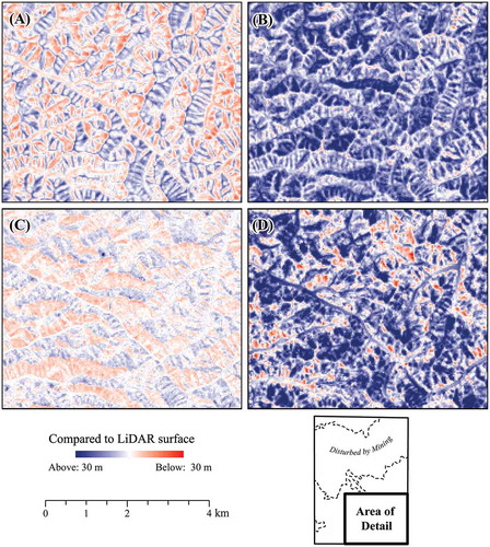
Figure 2 displays the absolute value error raster for each DEM on a consistent red to blue color ramp, where red shows negative error values indicating where the DEM is below the reference surface and blue shows positive error values indicating where the DEM is above the reference surface. This figure shows a subarea of the full study extent to allow for large-scale visualization of the differences. From this visualization, it is apparent that the DLGDEM and SAMBDEM (Figure 2A and 2D, respectively) have the lowest overall error, and that the SRTMDEM and GDEM (Figure 2B and 2D, respectively) have comparatively large and mostly positive error. For the DLGDEM and SAMBDEM, error appears to be higher on the sides of mountain ridges and lower in valleys. This expected correlation of slope and error is less visually prominent in the SRTM and GDEM rasters, possibly due to a higher impact of other factors such as layover and foreshortening in the former and pixel-mismatch in the latter.

Figure 2. Error rasters generated from the LiDARDEM minus each DEM calculation. (A) LiDAR – DLGDEM; (B) LiDAR – SRTMDEM; (C) LiDAR – GDEM; (D) LiDAR – SAMBDEM.

The elevation data sources evaluated here (photogrammetry, IFSAR, and LiDAR) detect topography in different ways, and thus the model of the topographic surface produced from each differs. This idea is well documented by previous studies (Bolstad and Stowe 1994; Kienzle 2004; Carlisle 2005; Fisher and Tate 2006; Li and Wong 2010), and the findings of this study further support this understanding. The question that remains is how comparable are regional and global DEMs, and what uncertainties need to be considered when they are directly compared. Additionally, DEM error has been found to be correlated with relief and slope (Bolstad and Stowe 1994; Carlisle 2005; Gómez et al. 2012). The quantitative analysis results attempt to explore these issues.

Table 2 displays OLS results for elevation and error, and for slope and error. These results support the qualitatively observed correlation between error and elevation and between error and slope. However, the impact of these two variables differs in magnitude and in the direction of error (positive or negative) for each DEM. For the DLGDEM, error is positively related to elevation (valleys have low error, while peaks and ridges have higher error) and slope (steep slopes have higher error). In the case of elevation, this relationship is statistically significant. The SRTMDEM exhibits similar relationships, with both elevation and slope being significantly and positively associated with error. By comparison, the GDEM shows a significant relationship with slope, but this relationship is negative, suggesting that flatter slopes have higher error values. This relationship is likely an artifact of the interaction of local topography and land use – relatively flat areas are mostly confined to narrow valley bottoms, which are also the sites of most residential or industrial development in this area. Though the total area associated with industrial and residential land use is relatively small in the study area, problems due to roof elevations being included in the DEM will be concentrated in this part of the landscape. Other studies have found that high errors in the GDEM, though not limited to flat areas as seen in this study, are caused by the inclusion of multiple image dates in the photogrammetric DEM extraction. Though the use of multiple image dates maximizes cloud-free areas in the imagery, it also introduces errors in geometric alignment and mismatched pixels (Chirico, Malpeli, and Trimble 2012). Aspect and error were significantly correlated in all DEMs except the SAMBDEM; however, the impact of aspect is substantially lower than elevation or slope, as suggested by the lower R² values (Table 2). It was expected that aspect would be significantly correlated with error in the SRTMDEM, as IFSAR elevation correction has an inherent directionality and known directional errors (such as layover and foreshadowing). However, the similar correlation of aspect and error in the DLGDEM was not expected. This correlation may be caused by distortion introduced by the flight direction of the aerial imagery or the semi-automation of photogrammetric DEM extraction. Overall, the very low R² values for all DEMs suggest that, though the relationships between error and elevation, error and slope, and error and aspect are significant, the three variables do not explain much of the error present in each of the evaluated DEMs. At the very least, the mixed OLS regression results point to the complexity of the relationship between error and these variables, and again highlight the differences between DEM datasets.

Table 2. OLS regression of elevation and error, slope and error, and aspect and error. There is a positive, significant relationship between elevation and error in the DLGDEM and SRTMDEM and between slope and error in the SRTMDEM.

Variables	Metric	DLGDEM	SRTMDEM	SAMBDEM	GDEM
Elevation and error
	R^2	0.048	0.020	0.003	0.001
	p > |t|	<0.0001*	<0.0001*	0.064	0.425
	Coefficient	0.024	0.021	0.003	0.005
Slope and error
	R^2	0.002	0.038	0.005	0.009
	p > |t|	0.165	<0.0001*	0.034*	0.004*
	Coefficient	0.036	0.021	0.030	−0.146
Aspect and error
	R^2	0.001	0.001	0.0001	0.0001
	p > |t|	<0.0001*	<0.0001*	0.219	<0.0001*
	Coefficient	1.233	−13.142	−0.177	−12.943

Notes: no significance (ns): p > 0.05, *p ≤ 0.05, ** p ≤ 0.01, *** p ≤ 0.001, **** p ≤ 0.0001.

The descriptive statistics of error values by land cover class are shown in Table 3. From this table, it is clear that error in all DEMs is impacted by land cover, but the specific relationships between error and land cover are DEM-specific. In general, all DEMs exhibit large minimum and maximum values in the forest and developed land cover classes. Though this is not unexpected, the magnitude of the outliers in the forest class is interesting. Both the DLGDEM and SAMBDEM, which maintain low average errors in all land covers, have substantially larger minimum and maximum errors in forest land cover. This suggests that forest land cover is correlated with outlier error values that exist many meters above and below the reference elevation surface. The DLGDEM and SAMBDEM should be the least impacted by vegetation, because they are collected during leaf-off seasons. For the SRTM, these results support the findings of Hofton et al. (2006), and indicate an average error in forested land cover that places the SRTMDEM surface somewhere between the ground and the canopy’s reflective surface. All DEMs except the SAMBDEM exhibit large minimum error values for developed land cover, suggesting a surface above the reference surface. As noted above, land cover, slope, aspect, and elevation jointly contribute to error in complex, sometimes unpredictable, ways. Though developed land cover generally occurs on low slopes, the majority of developed land in the study area is confined to a four-lane highway with steeply sloping sides. This unusual situation may result in the large outlier values in the developed land cover class, particularly for the SRTMDEM and the GDEM.

Table 3. Descriptive statistics of the error values in meters for each DEM, broken out by land cover.

	Land Cover	Developed	Forest	Grassland/pasture	Shrub/crop
DLG	Minimum	−10.33	−17.59	−15.46	1.11
	Maximum	13.43	22.98	9.15	15.56
	Mean	−0.95	1.76	−0.88	8.34
	Standard deviation	5.74	5.95	4.64	10.22
SRTM	Minimum	−29.44	−36.17	−24.51	−6.20
	Maximum	3.40	9.59	2.42	−1.38
	Mean	−13.36	−12.76	−8.84	−3.79
	Standard deviation	6.66	8.01	6.33	3.41
SAMB	Minimum	−5.62	−20.95	−4.15	−0.69
	Maximum	7.50	13.00	5.85	5.85
	Mean	−0.33	0.28	0.21	2.58
	Standard deviation	3.10	3.09	2.32	4.62
GDEM	Minimum	−24.22	−49.19	−22.27	−10.65
	Maximum	9.98	24.28	12.59	−5.72
	Mean	−7.06	−12.73	−3.49	−8.19
	Standard deviation	8.95	11.41	8.57	3.48

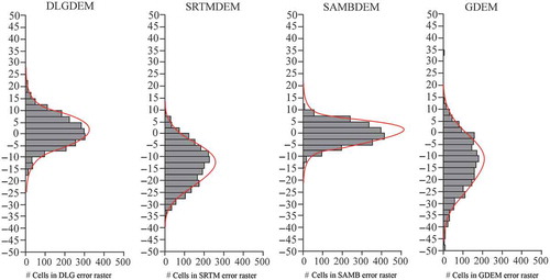
The histograms of the error values for each DEM, shown in Figure 3, provide an enhanced understanding of the amount and numeric distribution of error in each DEM (Höhle and Höhle 2009). Histograms are shown with uniform scaling to allow for direct comparison, and there is a marked difference in the error distribution of each DEM. As initially observed in Figure 2, the majority of SRTMDEM and GDEM error values lie below zero, indicating that the corresponding areas of the DEM are above the reference topographic surface. This is partially explained by their collection methods, which generally detect the upper surface of the forest canopy, and thus a surface that is not representative of a bare earth surface. Other studies have similarly observed the GDEM, both first and second versions, to have a negative bias on a global scale (Slater et al. 2011; Hirt, Filmer, and Featherstone 2010). Though the season of data collection, whether during leaf-on or leaf-off, might introduce error, all DEMs evaluated were collected during leaf-off season (see Table 1), minimizing this as a potential source of error.

Figure 3. Histograms of the number of grid cells with values in increments of 5 m, for each DEM.

Descriptive statistics of the error values for each DEM are shown in Table 4, and provide a quantitative comparison of the DEMs. A highly accurate DEM will exhibit a small minimum–maximum range, a normal unimodal distribution with a mean near zero, low skewness, a high p-value of the W test, a low RMSE, a low mean error, a low standard deviation, and a low t-score (Daniel and Tennant 2007). The following sections describe each DEM in terms of its errors, with the order of the DEMs discussed proceeding from lowest to highest overall DEM error.

Table 4. Statistical measures of each error raster. Error rasters with a non-normal distribution are highlighted in gray; however, both normal and non-normal measures are calculated for all error rasters. While the majority of these statistical measures utilize the signed difference in elevation between the reference surface and the tested DEM surface (indicated by ∆h), the non-normal error distribution measures of the 68.3 percentile and the 95th percentile show the absolute value of the errors (indicated by ).

			SAMBDEM	DLGDEM	SRTMDEM	GDEM
Descriptive statistic	Maximum	∆h	13.00	22.98	9.59	24.28
	Minimum	∆h	−20.96	−17.59	−36.17	−49.19
		∆h	0.25	1.66	−12.59	−12.17
	Skewness	∆h	−0.123	0.136	0.016	−0.078
Test for normalcy	W-score					0.99^ns
	t-Score
Normal distribution measure	RMSE (m)	∆h	3.05	6.14	14.90	16.77
	Mean error	∆h	0.25	1.69	−12.59	−12.17
	Σ	∆h	3.04	5.91	7.97	11.54
Non-normal error distribution measure	Median (50%)	∆h	0.14	1.44	−12.74	−12.14
	NMAD	∆h	2.81	5.77	8.28	11.81
	68.3%		2.81	6.08	16.49	17.86
	95%		5.83	12.50	25.57	31.76

Notes: ns: p > 0.05, *p ≤ 0.05, **p ≤ 0.01, ***p ≤ 0.001, ****p ≤ 0.0001.

The SAMBDEM had the lowest errors of all evaluated datasets within the study area. Its error value histogram exhibited the smallest range, with the mode centered near zero. However, the W test, based on a null hypothesis of error values being normally distributed, was rejected at the 0.01% significance level (p < 0.0001). This demonstrates that the error value distribution is not normal, and thus non-normal tests were used to further assess the distribution of its values. A low standard deviation and a low t-score of 2.567, significant at the 5% level (p < 0.05), indicate that the majority of error values are close to the mean, which is significantly different from zero. The NMAD is lower for the SAMBDEM than for other DEMs. This, in conjunction with the comparatively low value of the 95% quartile measure, confirms that the SAMBDEM is the most accurate elevation dataset evaluated.

The DLGDEM also showed low error values within the study area. Its histogram exhibits a unimodal distribution with a small range and small standard deviation, centered near zero. These factors indicate low overall error in the DEM and few outliers. The W test for the DLGDEM, based on a null hypothesis of the error values being normally distributed, was not significant, which leads to an assumption of normality of the error value distribution. A highly significant t-score indicates that the sample mean is significantly different from zero, possibly indicating systematic bias in the error values. However, a comparatively low RMSE, low mean error, low NMAD value, and low 95% quartile support the conclusion of low errors overall in the dataset.

From the histogram, it is evident that error values in the SRTMDEM are generally much larger and have a wider spread around the mean than those of the SAMBDEM and DLGDEM. As noted above, the peak of this histogram is centered substantially below zero, the sample mean is significantly different from zero, and has a t-score of −49.957 (p < 0.0001). The W test suggests that error values have a normal distribution. These factors indicate that the topographic surface of the SRTMDEM lies above the reference surface. This is not unusual in a DEM created from C-band IFSAR, which is impacted by dense vegetation and may not reach the ground. The 12.59 m negative offset of the sample mean (indicating a modelled surface 12.59 m above the reference surface) is likely caused by the dense deciduous forest (of approximately the same height) that grows in the region (see Miliaresis and Delikaraoglou 2009 for a discussion on the effect of forest on the SRTM). Despite the higher degree of error within the DEM and the vertical offset of the modelled topographic surface, the SRTMDEM is valuable for topographic change detection and analysis because it provides information not otherwise available during the 27-year time span between the collection dates of the DLGDEM and the SAMBDEM.

Error values associated with the GDEM were similar in range and magnitude to those associated with the SRTMDEM. Like the SRTMDEM, the GDEM histogram peaks well below zero and has a t-score which confirms that the mean is significantly different from zero. These two factors indicate that the modelled topographic surface lies above the reference DEM surface. The W test was not rejected (p < 0.59), suggesting that all statistical tests that assume normality are valid for the GDEM error. Despite its similarities to the SRTMDEM in magnitude and distribution of error values, the GDEM is fundamentally different from the other photogrammetric DEMs in its inclusion of multiple image dates for the elevation data extraction. This results in an inconsistent elevation surface in areas of dynamic topography and uncertainty regarding the specific associated date of the elevation at each pixel location.

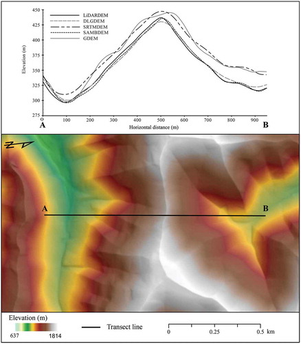
Qualitatively and quantitatively, the error rasters of the four compared DEMs exhibit substantial differences. These are clearly visible in a cross-sectional profile of a mountain ridge in the study area, shown in Figure 4. From this figure, it is clear that the DLGDEM and the SAMBDEM most closely approximate the LiDAR reference DEM, and that the GDEM and SRTMDEM, while modelling a similar surface, greatly overpredict the reference surface.

Figure 4. Comparisons of the DEM along a transect across a ridge.

This has direct implications for topographic change detection through DEM comparison. When analyzed at the 7.5′ topographic quadrangle extent, the DLGDEM and SAMBDEM are conceptually comparable and overall exhibit low vertical error compared to the LiDARDEM. However, these three datasets cannot be compared at regional scales due to limitations in their collection extents (recall that DLGs are available for the entire United States, but were collected by 7.5′ quadrangle and thus the collection year may differ at quadrangle boundaries; the SAMBDEM is a state-wide DEM, and the LiDARDEM is collected for part of southern WV). Based on the extent of their source data and the similarity of their modelled surfaces (see Figure 4), the GDEM and SRTMDEM are the only datasets that should be compared in regional studies. However, the GDEM is not associated with a specific moment in time, limiting its use in the quantification of topographic change, particularly in geomorphically dynamic areas.

When, as in this situation, it becomes necessary to ‘make the best’ of available data, it is still important to consider the specific application of topographic change analysis. For many such analyses, the potential errors of a dataset are larger than the amount of topographic change that is expected. For example, in a study of road cuts and fills, the potential elevation change is generally small, so the 12.9 m RMSE of the SRTM data might overwhelm any real changes. However, in a study of surface mining, the potential elevation change is very large, so it is possible that SRTM data, despite its large RMSE, could be compared to SAMB data with meaningful results.

Preprocessing of the SRTM data to bring the median error value from −12.74 m (above the ground) to 0 (ground surface) through a global offset would make the dataset more comparable to the SAMB data. Visual analysis of each DEM histograms and the DEM of difference should be used to inform such preprocessing methods. Additional preprocessing methods to filter substantial anomalies from a DEM may be necessary to make the two elevation surfaces comparable (Gesch 2014). Regardless of their statistical similarity, all topographic change quantification should include discussion of the error potentially included in the detected change.

Since all DEMs were found to have normal, or near-normal error distributions in this study, the RMSE value may be used as an approximation of error. However, the selection of this metric is heavily dependent on the distribution of error values. A non-normal distribution would require the use of a non-normal metric, such as the NMAD. Furthermore, in order to directly compare two DEMs, it is necessary to incorporate the potential error of both, and in many cases, this combination of error may overwhelm the actual topographic change to be quantified. For example, if a comparison is made between the DLGDEM and the SRTMDEM, the possible error at each pixel is as high as 21.04 m – roughly the height of a seven-storey building. Thus, for some combinations of DEMs, such as the GDEM and the SRTMDEM, ‘topographic change’ becomes meaningless because it must include a potential error of 31.67 m. The user is left to determine the threshold of unacceptably high error appropriate for the comparison application.

Conclusion

This study compared several regional- and global-scale DEMs to a high-accuracy LiDAR DEM to quantitatively and qualitatively assess their differences in the rugged topography of the southern WV coalfields. These DEMs included a grid interpolated from USGS 7.5′ topographic map DLGs, the SRTM, a state-wide photogrammetric DEM (the SAMB), and the ASTER GDEM. Each DEM was compared to the LiDARDEM by grid differencing and the resultant ‘error’ values were analyzed using various statistical measurements. In general, these datasets form two groups: one with relatively high accuracy and another with relatively low accuracy. The high-accuracy group comprises the SAMBDEM and the DLGDEM, with RMSE values of 3.05 m and 6.14 m, respectively, and the low-accuracy group is comprised of the SRTMDEM and GDEM, with RMSE values of 14.90 m and 16.77 m, respectively. Though the RMSE value suggests a quick, global figure representing the accuracy of each DEM, a more comprehensive understanding of each DEM’s representation of the topographic surface is gained through evaluation and comparison of other statistical values, such as basic descriptive statistics, histograms, and tests for normalcy. OLS regression provides insight regarding the complex relationships among elevation, slope, and error. These values suggest that both the SRTMDEM and the GDEM describe a topographic surface substantially above that modelled by the LiDARDEM. The GDEM suffers from a further problem for use in areas with rapidly changing elevations, in that the modelled surface does not represent a single snapshot in time, but instead imagery acquired over an extended period. This problem may preclude the use of the GDEM in elevation change-detection studies. Future research will focus on methods for incorporating these measures of DEM inaccuracy into specific values, to be added or subtracted from topographic change-detection quantifications, as well as to methods that incorporate these uncertainties in topographic change products.

Disclosure statement

No potential conflict of interest was reported by the authors.

Acknowledgments

The views and conclusions contained in this document are those of the authors and should not be interpreted as representing the opinions or policies of the US Government. Mention of trade names or commercial products does not constitute their endorsement by the US Government.

Additional information

Funding

The project described in this publication was supported in part by the United States Geological Survey to AmericaView [grant agreement number G14AP00002].

References

- Abrams, M., B. Bailey, H. Tsu, and M. Hato. 2010. “The ASTER Global DEM.” Photogrammetric Engineering and Remote Sensing 76 (4): 344–348.
- Aguilar, F. J., F. Agüera, M. A. Aguilar, and F. Carvajal. 2005. “Effects of Terrain Morphology, Sampling Density, and Interpolation Methods on Grid DEM Accuracy.” Photogrammetric Engineering & Remote Sensing 71 (7): 805–816.
- ASTER GDEM Validation Team. 2011. “ASTER Global Digital Elevation Model Version 2 Summary Report.” Accessed July 15, 2014. https://lpdaacaster.cr.usgs.gov/GDEM/Summary_GDEM2_validation_report_final.pdf
- Blanchard, S. D., J. Rogan, and D. W. Woodcock. 2010. “Geomorphic Change Analysis Using ASTER and SRTM Digital Elevation Models in Central Massachusetts, USA.” GIScience & Remote Sensing 47 (1): 1–24. doi:10.2747/1548-1603.47.1.1.
- Bolstad, P. V., and T. Stowe. 1994. “An Evaluation of DEM Accuracy: Elevation, Slope, and Aspect.” Photogrammetric Engineering & Remote Sensing 60 (11): 1327–1332.
- Carlisle, B. H. 2005. “Modelling the Spatial Distribution of DEM Error.” Transactions in GIS 9 (4): 521–540. doi:10.1111/j.1467-9671.2005.00233.x.
- Chaplot, V., F. Darboux, H. Bourennane, S. Leguédois, N. Silvera, and K. Phachomphon. 2006. “Accuracy of Interpolation Techniques for the Derivation of Digital Elevation Models in Relation to Landform Types and Data Density.” Geomorphology 77 (1): 126–141.
- Chirico, P. G., K. C. Malpeli, and S. M. Trimble. 2012. “Accuracy Evaluation of an ASTER-Derived Global Digital Elevation Model (GDEM) Version 1 and Version 2 for Two Sites in Western Africa.” GIScience & Remote Sensing 49: 775–801. doi:10.2747/1548-1603.49.6.775.
- Chu, H., C. Wang, M. Huang, C. Lee, C. Liu, and C. Lin. 2014. “Effect of Point Density and Interpolation of Lidar-Derived High-Resolution Dems on Landscape Scarp Identification.” GIScience & Remote Sensing 51 (6): 731–747. doi:10.1080/15481603.2014.980086.
- Daniel, C., and K. Tennant. 2007. “DEM Quality Assessment, Digital Elevation Model Technologies and Applications.” Chapter 12. In The DEM User’s Manual, edited by D. F. Maune, 395–440. Bethesda, MD: ASPRS.
- DiCicco, S. 2011. “RAMPP WV Coal River QA/QC Report.” Memorandum. Accessed July 15, 2014. http://www.wvview.org/data/lidar/SouthernWV/Metadata%20and%20Tiling%20Scheme/RAMPP_WV_Memo_20110722_Final.pdf
- Evans, R. T., and H. M. Frye. 2009. History of the Topographic Branch (Division). Reston, VA: U.S. Geological Survey Circular.
- Fedorko, E. J. 2005. “An Accuracy Assessment of SAMB Elevation Data.” Report. Accessed 2013. West Virginia Technical Center. http://www.wvgis.wvu.edu
- Fisher, P. F., and N. J. Tate. 2006. “Causes and Consequences of Error in Digital Elevation Models.” Progress in Physical Geography 30 (4): 467–489. doi:10.1191/0309133306pp492ra.
- Fowler, R. 2007. “Topographic Lidar, Digital Elevation Model Technologies and Applications.” Chapter 7. In The DEM User’s Manual, edited by D. F. Maune, 207–236. Bethesda, MD: ASPRS.
- Gesch, D. 2005. “Analysis of Multi-Temporal Geospatial Data Sets to Assess the Landscape Effects of Surface Mining.” Proceedings of the 22nd Annual National Conference of the American Society of Mining and Reclamation, Breckenridge, CO, June 19–23.
- Gesch, D. 2014. “An Inventory of Topographic Surface Changes: The Value of Multi-Temporal Elevation Data for Change Analysis and Monitoring.” ISPRS-International Archives of the Photogrammetry, Remote Sensing, and Spatial Information Sciences XL-4: 59–63. doi:10.5194/isprsarchives-XL-4-59-2014.
- Gesch, D., M. Oimoen, Z. Zhang, D. Meyer, and J. Danielson. 2012 “Validation of the ASTER Global Digital Elevation Model Version 2 Over the Conterminous United States.” International Archives of the Photogrammetry, Remote Sensing and Spatial Information Sciences. Vol. 34–B4, Melbourne, Australia, 22 ISPRS Congress, August 25–September 1.
- Gómez, M. F., J. D. Lencinas, A. Siebert, and G. M. Díaz. 2012. “Accuracy Assessment of ASTER and SRTM Dems: A Case Study in Andean Patagonia.” GIScience & Remote Sensing 49 (1): 71–91. doi:10.2747/1548-1603.49.1.71.
- Gong, J., Z. Li, Q. Zhu, H. Sui, and Y. Zhou. 2000. “Effects of Various Factors on the Accuracy of Dems: An Intensive Experimental Investigation.” Photogrammetric Engineering & Remote Sensing 66 (9): 1113–1117.
- Gonga-Saholiariliva, N., Y. Gunnell, C. Petit, and C. Mering. 2011. “Techniques for Quantifying the Accuracy of Gridded Elevation Models and for Mapping Uncertainty in Digital Terrain Analysis.” Progress in Physical Geography 35: 739–764. doi:10.1177/0309133311409086.
- Guth, P. L. 2006. “Geomorphometry from SRTM: Comparison to NED.” Photogrammetric Engineering and Remote Sensing 72 (3): 269–277. doi:10.14358/PERS.72.3.269.
- Hengl, T., and I. S. Evans. 2009. “Chapter 2 Mathematical and Digital Models of the Land Surface.” In Geomorphometry: Concepts Software, Applications, edited by T. Hengl and H. I. Reuter, 31–63. Amsterdam: Elsevier. 10.1016/S0166-2481(08)00002-0.
- Hensley, S., R. Munjy, and P. Rosen. 2007. “Interferometric Synthetic Aperture Radar (IFSAR), Digital Elevation Model Technologies and Applications.” Chapter 6. In The DEM User’s Manual, edited by D. F. Maune, 142–206. Bethesda, MD: ASPRS.
- Hicks, M. 2012. “Remotely Sensed Topographic Change in Gravel Riverbeds with Flowing Channels.” Chapter 23. In Gravel-Bed Rivers: Processes Tools, Environments, edited by M. Church, B. Pascale, and A. Roy, 303–314. West Sussex: Wiley-Blackwell.
- Hirano, A., R. Welch, and H. Lang. 2003. “Mapping from ASTER Stereo Image Data: DEM Validation and Accuracy Assessment.” ISPRS Journal of Photogrammetry and Remote Sensing 57 (5–6): 356–370. doi:10.1016/S0924-2716(02)00164-8.
- Hirt, C., M. Filmer, and W. Featherstone. 2010. “Comparison and Validation of the Recent Freely Available ASTER-GDEM Ver1, SRTM Ver4.1 and GEODATA DEM-9S Ver3 Digital Elevation Models over Australia.” Australian Journal of Earth Sciences 57 (3): 337–347. doi:10.1080/08120091003677553.
- Hodgson, M. E., J. Jensen, L. Schmidt, S. Schill, and B. A. Davis. 2003. “An Evaluation of LIDAR- and IFSAR- Derived Digital Elevation Models in Leaf-On Conditions with USGS Level 1 and Level 2 Dems.” Remote Sensing of Environment 84 (2): 295–308. doi:10.1016/S0034-4257(02)00114-1.
- Hoffmann, J., and D. Walter. 2006. “How Complementary are SRTM-X and –C Band Digital Elevation Models?” Photogrammetric Engineering & Remote Sensing 72 (3): 261–268. doi:10.14358/PERS.72.3.261.
- Hofton, M., R. Dubayah, J. B. Blair, and D. Rabine. 2006. “Validation of SRTM Elevations over Vegetated and Non-Vegetated Terrain Using Medium Footprint Lidar.” Photogrammetric Engineering & Remote Sensing 72 (3): 279–285. doi:10.14358/PERS.72.3.279.
- Höhle, J., and M. Höhle. 2009. “Accuracy Assessment of Digital Elevation Models by Means of Robust Statistical Methods.” ISPRS Journal of Photogrammetry and Remote Sensing 64 (4): 398–406. doi:10.1016/j.isprsjprs.2009.02.003.
- Hooke, R. 1999. “Spatial Distribution of Human Geomorphic Activity in the United States: Comparison with Rivers.” Earth Surface Processes and Landforms 24 (8): 687–692.
- Hooke, R. 2000. “On the History of Humans as Geomorphic Agents.” Geology 28 (9): 843–846. doi:10.1130/0091-7613(2000)28<843:OTHOHA>2.0.CO;2.
- Huggel, C., D. Schneider, P. Julio Miranda, H. DelgadoGranados, and A. Kääb. 2008. “Evaluation of ASTER and STRM DEM Data for Lahar Modeling: A Case Study on Lahars from Popocatépetl Volcano, Mexico.” Journal of Volcanology and Geothermal Research 170: 99–110. doi:10.1016/j.jvolgeores.2007.09.005.
- Hutchinson, M. 1988. “Calculation of Hydrologically Sound Digital Elevation Models.” Proceedings of the Third International Symposium on Spatial Data Handling, Sydney, August 17–19.
- Hutchinson, M. 1989. “A New Procedure for Gridding Elevation and Stream Line Data with Automatic Removal of Spurious Pits.” Journal of Hydrology 106 (3–4): 211–232. doi:10.1016/0022-1694(89)90073-5.
- Hutchinson, M. F. 2006. ANUDEM Version 5.2 User Guide. Canberra: Fenner School of Environment and Society, Australian National University.
- James, L. A., M. E. Hodgson, S. Ghoshal, and M. M. Latiolais. 2012. “Geomorphic Change Detection Using Historic Maps and DEM Differencing: The Temporal Dimension of Geospatial Analysis.” Geomorphology 137 (1): 181–198. doi:10.1016/j.geomorph.2010.10.039.
- Jensen, J. R. 2007. Remote Sensing of the Environment. Upper Saddle River, NJ: Prentice Hall.
- Kanji, G. K. 2006. 100 Statistical Tests. 3rd ed. Thousand Oaks, CA: Sage.
- Khalsa, S. J. S., M. B. Dyurgerov, T. Khromova, B. H. Raup, and R. G. Barry. 2004. “Space-Based Mapping of Glacier Changes Using ASTER and GIS Tools.” IEEE Transactions on Geoscience and Remote Sensing 42 (10): 2177–2183. doi:10.1109/TGRS.2004.834636.
- Kienzle, S. 2004. “The Effect of DEM Raster Resolution on First Order, Second Order and Compound Terrain Derivatives.” Transactions in GIS 8: 83–111. doi:10.1111/j.1467-9671.2004.00169.x.
- Li, J., and D. W. S. Wong. 2010. “Effects of DEM Sources on Hydrologic Applications.” Computers Environment and Urban Systems 34: 251–261. doi:10.1016/j.compenvurbsys.2009.11.002.
- Martı́nez-Casasnovas, J. A., M. C. Ramos, and J. Poesen. 2004. “Assessment of Sidewall Erosion in Large Gullies Using Multi-Temporal Dems and Logistic Regression Analysis.” Geomorphology 58: 305–321. doi:10.1016/j.geomorph.2003.08.005.
- Miliaresis, G., and D. Delikaraoglou. 2009. “Effects of Percent Tree Canopy Density and DEM Misregistration on SRTM/NED Vegetation Height Estimates.” Remote Sensing 1: 36–49. doi:10.3390/rs1020036.
- Molander, C. W. 2001. “Photogrammetry, Digital Elevation Model Technologies and Applications.” Chapter 5. In The DEM User’s Manual, edited by D. F. Maune, 121–141. Bethesda, MD: ASPRS.
- Passini, R., K. Jacobsen, and R. M. Passini. 2007. “Accuracy Analysis of SRTM Height Models.” Proceedings of ASPRS Annual Conference, Tampa, FL, May 7–11, 25–29.
- Phillips, J. 2004. “Impacts of Surface Mine Valley Fills on Headwater Floods in Eastern Kentucky.” Environmental Geology 45 (3): 367–380. doi:10.1007/s00254-003-0883-1.
- Pierce, L., J. Kellndorf, W. Walker, and O. Barros. 2006. “Evaluation of the Horizontal Resolution of SRTM Elevation Data.” Photogrammetric Engineering & Remote Sensing 72 (11): 1235–1244. doi:10.14358/PERS.72.11.1235.
- Ren, Z., Z. Zhang, F. Dai, J. Yin, and H. Zhang. 2014. “Topographic Changes Due to the 2008 Mw 7.9 Wenchuan Earthquake as Revealed by the Differential DEM Method.” Geomorphology 217: 122–130. doi:10.1016/j.geomorph.2014.04.020.
- Rodríguez, E., C. S. Morris, and J. E. Belz. 2006. “A Global Assessment of the SRTM Performance.” Photogrammetric Engineering & Remote Sensing 72 (3): 249–260. doi:10.14358/PERS.72.3.249.
- Rogerson, P. 2006. Statistical Methods for Geography: A Student’s Guide. 1st ed. Thousand Oaks, CA: SAGE Publications.
- Rosette, J., J. Suárez, R. Nelson, S. Los, B. Cook, and P. North. 2012. “Lidar Remote Sensing for Biomass Assessment.” In Remote Sensing of Biomass - Principles and Applications, edited by L. Fatoyinbo, 3–26. Rijeka: InTech.
- Slater, J. A., B. Heady, G. Kroenung, W. Curtis, J. Haase, D. Hoegemann, C. Shockley, and K. Tracy. 2011. “Global Assessment of the New ASTER Global Digital Elevation Model.” Photogrammetric Engineering and Remote Sensing 77 (4): 335–349. doi:10.14358/PERS.77.4.335.
- USGS (U.S. Geological Survey). 1993. “Data Users Guide 5: Digital Elevation Models.” Reston, VA: U.S. Geological Survey. http://pubs.usgs.gov/of/2003/0017/sus_met.txt
- USGS (U.S. Geological Survey). 2006. “Map Accuracy Standards Fact Sheet FS-171-99.” Accessed July 1, 2014. http://pubs.usgs.gov/fs/1999/0171/report.pdf
- USGS (U.S. Geological Survey). 2009. “SRTM Topography.” SRTM Documentation, 2.1. Accessed July 14, 2014. http://dds.cr.usgs.gov/srtm/version_1/Documentation/SRTM_Topo.pdf
- USGS (U.S. Geological Survey). 2013. “USGS Topographic Maps.” Accessed May 1. http://nationalmap.gov/
- Wechsler, S., and C. Kroll. 2006. “Quantifying DEM Uncertainty and its Effect on Topographic Parameters.” Photogrammetric Engineering & Remote Sensing 72: 1081–1090. doi:10.14358/PERS.72.9.1081.
- Weng, Q. 2002. “Quantifying Uncertainty of Digital Elevation Models Derived from Topographic Maps.” In Advances in Spatial Data Handling, edited by D. E. Richardson and P. Van Oosterom, 403–418. Berlin: Springer.
- WVDHSEM (West Virginia Division of Homeland Security and Emergency Management). 2014. “Statewide Addressing and Mapping.” Accessed December 3. http://www.dhsem.wv.gov/gis/Pages/default.aspx
- Wheaton, J. M., J. Brasington, S. E. Darby, and D. Sear. 2009. “Accounting for Uncertainty in Dems from Repeat Topographic Surveys: Improved Sediment Budgets.” Earth Surface Processes and Landforms 35 (2): 136–156.