Floodplain wetland mapping in the White Volta River Basin of Ghana

Abstract

Apart from the earmarked Ramsar sites along the coastal zones of Ghana, no inventory has been conducted to determine the location, distribution, and status of wetlands within any of its river basins. In this study, a logistic regression model was used within the GIS platform to predict, at pixel level, the presence of a wetland in the basin of the White Volta River. The output consisted of a map and also indicated that a total of 259.5 km² of the land mass is estimated as probable floodplain wetland sites. The model used resulted in a high level of accuracy in predicting wetland presence.

Keywords:

• floodplain
• Wetland
• logistic regression
• mapping

1. Introduction

In recent times, wetland systems on floodplains have gained much recognition and value. One reason, among others, is that they contribute to a healthy ecology and retain water. Also, many endangered species depend on these wetland systems (Mitsch and Gosselink 2000; May et al. 2002). To accurately map wetland sites on floodplains within a river basin, researchers have relied on tried and tested spatial and multivariate statistical techniques. Results generated by spatial and multivariate statistical techniques provide sufficient information to assist decision-makers/environmentalists to understand, evaluate, monitor, and manage the effects of human activities on wetland systems. Methods used by agencies and researchers to delineate and extract wetland data are often questioned on the basis that they are debatable and very difficult to validate and apply in many environmental settings (Dewey et al. 2006). In an attempt to resolve the controversy over wetland delineation, the United States National Research Council, Ramsar Convention, and other agencies have provided a definition of wetlands (Ramsar 2004). To confirm the existence of wetlands, three main indicators should emerge: hydric soil, wetland hydrology, and hydrophytic vegetation (Dewey et al. 2006). However, it is maintained that, for wetland delineation, long-term monitoring of surface and subsurface water is important, because in most situations hydric soil, hydrology, and hydrophytic indicators of wetlands rarely coincide (Wakeley, Sprecher, and Lichvar 1996).

Within the past few years, scientists have witnessed considerable developments in the application of spatial technologies to identify, map, and take inventories of resources in different landscapes, including wetlands on floodplains (Van De Giesen 2001; Harvey and Hill 2001; Ozesmi and Bauer 2002; Meijerink 2002; Jain et al. 2005; Lillesand, Kiefer, and Chipman 2008; Kumar and Sinha 2014). The use of multitemporal images has enhanced the ability of researchers to classify wetlands and separate them from other land cover classes. In the classification process, wetlands present further difficulties due to shallow water depth and the reflection of bottom sediments (Shaikh, Green, and Cross 2001). In such cases, the near-infrared (TM4, 0.7–0.9 μm) and mid-infrared (TM5, 1.55–1.75 μm) wavelengths of Landsat 7 ETM+ are superior to any others. At these wavelengths, shallow water absorbs, showing a greater tonal contrast in the infrared bands. Notably, optical remote sensing techniques alone may not be adequate to classify wetland regions on floodplains. However, radar sensors provide information on the quantity and distribution of water, irrespective of the weather conditions (Pope, Rey-Benayas, and Paris 1994; Dwivedi, Rao, and Bhattacharya 1999; Van De Giesen 2001).

Researchers have explored and combined Landsat images and ancillary data such as the normalized difference vegetation index (NDVI), spectral information, topographic index, and seasonality to identify, separate, and extract data about wetlands in different landscapes (Baker et al. 2006; Heinl et al. 2009). According to Merot et al. (2003), Phillips (1990), Chengmin and Lynn (2008), Guneralp, Filippi, and Hales (2013), and Kumar and Sinha (2014), when ancillary variables are incorporated into classification algorithms, the results correspond significantly to objects mapped in the field. Therefore, if ancillary data are incorporated into any spatial model, the ability of researchers to interpret and classify results is improved (Ricchetti 2000; Lersch, Haertel, and Shimabukuro 2007).

De Alwis et al. (2007), Wright and Gallant (2007), Islam et al. (2008), and Knight, Tindall, and Wilson (2009) have noted that saturated areas (wetlands) can be characterized with automated and semiautomated procedures on temporal sequences of Landsat 7 ETM+. In an attempt to use an automated procedure, Islam, Md et al. (2008) combined Landsat 7 ETM+ and the digital elevation model (DEM) from the Shuttle Radar Topographic Mission (SRTM-DEM). The results generated were spurious, with a high level of inconsistencies when compared with the location of the mapped sites. Also, Islam, Md et al. (2008) used a semiautomated approach, which involved displaying enhanced images through image rationing to distinguish and delineate wetlands from non-wetlands.

Geoscientists have combined multitemporal and ancillary data with rule-based classifiers such as object-oriented methods, decision trees, and artificial neural networks to reduce errors in wetland extraction on satellite images (Baker et al. 2006; Mladinich 2010; MacLean and Congalton 2011; Zhang et al. 2012; Tenenbaum, Yang, and Zhou 2011). To determine the occurrence or non-occurrence of object classes on an image (Sugumaran, Harken, and Gerjevic 2004), object-oriented procedure is relied on to overcome the limitation of pixel-based methods by combining both spatial and spectral information (Mladinich 2010). Object-oriented classification bridges the gap between geographic information system (GIS) data, sensor-derived parameters, and expert knowledge (Dekok et al. 1999; Tenenbaum, Yang, and Zhou 2011; Zhang, Xie, and Selch 2013). Decision tree classification has been used to extract data from satellite images, but it has been noted that a decision tree is unsuitable when feature space and training areas are changed (Rogan et al. 2008; Pooja, Jayanth, and Shivaprakash 2011).

Krishnapuram et al. (2005), Su and Huang (2009), Chen, Chen, and Son (2012) and Li, Im, and Beier (2013), noted that a family of algorithms, including sparse probit regression, relevance vector machine, information vector machine, and joint classifiers/feature optimization, can be applied to extract wetland data from digital satellite images. With training data, these algorithms learn as sparse classifiers with enhanced capability to distinguish between classes based on vector inputs (Qi, Zhao, and Feng 2010; Mahmood and Gloaguen 2011; Chen, Chen, and Son 2012; Aguirre-Salado et al. 2012).

Researchers have attempted to use multivariate analysis to extract spatial and temporal objects, such as wetlands, from satellite images (Krishnapuram et al. 2005; Mallinis and Koutsias 2008; Pantaleoni et al. 2009; Stoler et al. 2012; Panda et al. 2012). Mallinis and Koutsias (2008) and Pantaleoni et al. (2009) have observed that the use of multinomial logistic regression analysis to discriminate wetland types has challenges with accuracy; hence, such analysis cannot replace wetland delineation on high-resolution orthoimagery. However, they opine that applying an outlier detection technique using median and median absolute deviation to represent spectral reflectance characteristics of wetland class populations can generate wetland maps. The use of an outlier detection technique forms the basis for the calculation of the pixel change likelihood index. The individual likelihood index can be merged and converted to pixel change probability using a logistic regression (Nielsen, Prince, and Koeln 2008).

One of the goals of wetland scientists is to acquire a technique that can extract accurate wetland information. The conventional techniques such as image processing, field observation, and surveys used by researchers to study wetlands are time-consuming and differ in their results. This is because of inadequacies and constraints of the instruments they use, and differences in efficiencies of, and interpretation of data by, different researchers. Mapping wetlands using any form of image processing is challenging, due to the likelihood of spectral confusion between cover types. The use of automated methods produces spurious results. Multinomial logistic regression in wetland discrimination has challenges with accuracy. The use of models to extract wetland sites on floodplains is quite complicated because the explanatory variables have nonlinear relations with the response variables. On the contrary, a linear relationship between the response and explanatory variables is often required (Zhu and Huang 2006; Debella-Gilo and Etzelmüller 2009).

Apart from the earmarked Ramsar sites along the coastal zone in Ghana, there is no baseline data or comprehensive information on the types, status, distribution, and rates of change of floodplain wetlands within the White Volta River Basin. The conventional way of manually digitizing wetland maps on image is laborious and has a high production and updating cost. Additionally, the accuracies of supervised image classifiers such as spectral angle mapper and maximum likelihood are affected by factors such as nonuniformity of solar irradiation across scene due to topographical variation and similar spectral classes. Hence, there is a need to test how ancillary data could be combined within logistic regression model to improve the accuracy level of wetland mapping and updating. The objective of the study is to use spatial data to create a logistic regression equation and generate a wetland susceptibility map of the White Volta River floodplains. The research uses ancillary variables such as topography, climate, vegetation, and spatial and image parameters to predict probable wetland sites on floodplains. For wetland mapping within the White Volta River Basin, three main stages were adopted: (1) extraction of input data, (2) pixel sampling for wetland prediction, and (3) floodplain wetland extraction using logistic regression analysis.

2. Materials and methods

2.1. Study area

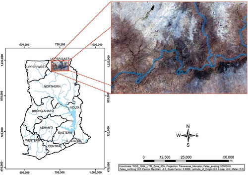
The study area covers about 8410 km² and is located in Ghana, specifically the Ghana section of the Volta River Basin (Figure 1). The entire White Volta Basin could not be studied because of the laborious and time-consuming bureaucratic procedure adopted by authorities in Burkina Faso and Togo, to secure permission to conduct ground truth. This site was selected because it has the potential in assisting farmers to locate areas with high residual soil moisture for dry season agricultural production. The climate of the study site is semiarid, and it is characterized by two major seasons: dry and rainy. In the dry season, Harmattan winds are dusty and dry, and they occur mostly from November to April (Nyarko 2007). In this semiarid climate, the annual potential evaporation is estimated to exceed annual precipitation. High evaporative values are recorded between November and April. Rainfall in this region begins in May and ends in October. The total annual rainfall is estimated at 1100 mm, with 301 mm recorded during the months of August and September.

Figure 1. Map of the study area in the White Volta River Basin. For full color versions of the figures in this paper, please see the online version.

The study area is underlain by the Voltaian system and Birimian granitoids (Kesse 1985). Soils found within the Volta River floodplain are eutric fluvisol, gleyic lixisols, eutric gleysols, and lithic leptosols. The contributions to subsurface water vary seasonally, and the volume of water in the entire wetland is a reflection of inflows relating to actual surface flux and groundwater recharge of 6 mm/day contributing to subsurface water (Nyarko 2007).

Vegetation found in the study site is characterized by interior wooded savannah (mid-dry savannah and wet savannah) and Guinea savannah (dry savannah). Tree species found in this vegetation zone include Mitragyna inermis, Combretum species, and Gardenia species. Also found are Pseudocedrela species, Afzelia africana, and Diospyros mespiliformis. Some grasses found include Andropogon gayanus var. bisquamulatus and Andropogon var. argyrophues, Pennisetum pedicellatum, and Hyparrhenia species. The vegetation of the study area has changed over the years as a result of human activities such as annual burning, cropping, grazing, and the felling of trees and shrubs during cultivation, giving it a heterogeneous cover characteristic.

2.2. Structure of the modeling process

The study combined software packages such as ILWIS 3.6, ENVI 4.7, and statistical package STATA 13 to develop a model that would generate probable wetland sites. The process of extracting floodplain wetland within the White Volta Basin was classified into three main automated stages. The first stage involved a combination of processes to generate different spatial layers (Table 1) from the Advanced Spaceborne Thermal Emission and Reflection Radiometer (ASTER), Global Digital Elevation Model (GDEM), Landsat images, and drainage networks. In the second stage, a random sampling procedure was applied to all layers within the ENVI 4.7 platform to extract data points as an input into STATA 13 for analysis. In the third stage, the extracted data points were used as input for the logistic regression model to extract wetlands on floodplain.

Table 1. Description of data used for floodplain wetland mapping.

Categories	Abbreviation	Explanatory variables	Units of measurement
Topographic	Slope	Slope	[Degrees]
	Shape index	Non-compactness of the landscape	[-]
	Wetness	Zone of saturation	[-]
	Power	Stream power index	[-]
	Elevation	Elevation data derived from the SRTM-DEM	[m]
	Internal	Internal relief	[m/km^2]
Environmental	NDVI	Normalized difference vegetation index	[-]
	SAVI	Soil adjusted vegetation index	[-]
	Geology	Geological formation	[-]
	Soil	Soil	[-]
Climatic	Evapo	Evapotranspiration calculated by SEBAL	[mm/day]
Image enhancement	Texture	Rugosity of the topography	[-]
	LogB4	Logarithm transformation of Band 4 of 30 October 2002 satellite image (wavelength λ of 0.77–0.90 µm)	[-]
Spatial	Distance	Distance estimated from the main river	[m]

Note: [-] refers to dimensionless quantity.

2.3. Input data and acquisition issues

Input data used to develop the logistic regression model are classified into five thematic areas (Table 1), these data are hydrologically divergent. These data were derived from sources such as (1) satellite image analysis, (2) a DEM from ASTER GDEM, (3) drainage networks obtained from the Survey Department of Ghana, (4) soil data from the Soil Research Institute, and (5) geology data from Ghana Geological Surveys.

To generate different data-sets for the study, a Landsat 7 ETM+ scene of the Ghana section of the White Volta River Basin dated 30 October 2002 was acquired, along the World Reference system (WRS-2) path-194 and row-53.

The researchers noted that the satellite image acquired had a different date from the period in which the fieldwork was conducted. Therefore, any form of data extracted from the image would not conform to the period within which the study was conducted. The image was used based on the views expressed by Jensen et al. (2009) that field validation of images should be near to the date of acquisition or the scheduled near anniversary. The near-anniversary concept is where images are acquired at approximately the same period in the year, when illumination and weather conditions at the site are likely to be most comparable. An examination of weather (sunshine hours) data from 2002 to 2005 indicated a high level of correlation of 0.92 between October 2002 and October 2004. The correlation between 2002 and 2005 data was 0.95 at a significance level of 0.05.

The ASTER GDEM with a spatial resolution of 30 m × 30 m is not error free; it contains artifacts that might have resulted from insufficient data or the interpolation technique adopted. Although not verified for Ghana, the ASTER GDEM has an accuracy of between 7 m and 14 m (ASTER Validation Team 2009).

2.3.1. Data processing

The selected satellite image was the clearest image after the rainy season. Additionally, wet conditions were captured, and it was sufficiently clear for visual identification of training samples. This image has been geometrically and radiometrically corrected (see Duadze 2004) and did not require any form of correction.

Many techniques have been developed to generate high-resolution DEMs that can capture various topographic variables within a land unit. Apart from the use of photographic methods, recently stereo satellite data (ASTER, STRM, and LiDAR) have been used to generate fine DEMs and reduce the effects of artifacts in them. Artifacts arise as a result of insufficient data or the interpolation technique adopted. To correct artifacts and extract topographic variables from a DEM, researchers have developed different algorithms that can be applied (Wilson, Lam, and Deng 2007; Lindsay and Evans 2008; Arnold 2010). There are no algorithms that can remove all artifacts from a DEM; the common algorithms used in software (for instance in ILWIS) to process DEMs have a variety of logical and computational procedures (Lindsay and Evans 2008; Arnold 2010). Within the ILWIS platform to minimize the errors in the DEM, three DEM filtering steps were applied before topographic parameters were derived: reduction of padi terraces, reduction of outliers, and incorporation of water bodies (Hengl, Gruber, and Shrestha 2003).

2.3.2. Land cover data extraction

To discriminate land cover classes from the satellite image, selected bands, i.e., near-infrared (band 4, wavelength λ of 0.77–0.90 µm), midinfrared (band 5, wavelength λ of 1.55–1.75 µm), and red (band 3, wavelength λ of 0.63–0.69 µm), were combined to generate a color composite image. The selected bands demonstrate moisture differences that showed levels of usefulness for analysis of soil and vegetation conditions (Lillesand, Kiefer, and Chipman 2008).

In 2004 and 2005, the basin was traversed and various land cover types and training areas (see Table 2) were marked on Google Earth images of 2004, complemented by aerial photographs of 2005 produced by the Survey Department of Ghana and hand-held GPS. The training area/sites were visited three times: at the beginning of the rainy season (in May), during the rainy season (in August), and at the end of the rainy season (in October). The classes marked on the field images were used for a supervised classification, in which the maximum likelihood classifier was adopted to generate seven cover classes (see Figure 2). In the classification process, a total of 30,000 training pixels (see Table 2) that corresponded to the ground truth were used to classify 9,344,303 pixels that constituted an image of the entire study area. Using a maximum likelihood method, a single probability threshold of 95% was specified for a pixel because the samples were randomly selected and an assumption of normal distribution of samples was made. Hence, pixels were assigned to a class if their probability exceeded the specific threshold.

Table 2. Land cover types in the study area and corresponding training areas.

Land cover type	Number of training plots/pixels
Wetlands	15/2 197
Waterbody	8/7 438
River	12/577
Forest	11/1 193
Open grassland	6/7 259
Bareland	4/5 567
Open forest	5/5 769

Figure 2. Land cover classes of part of the study area in upper east region, Ghana. For full color versions of the figures in this paper, please see the online version.

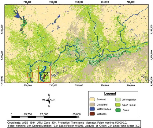
The accuracy of the land cover classification was assessed through field visits. The overall accuracy of land cover classification was estimated at 97.11% (see Table 3), indicating that classes specified are easily distinguishable. Producer accuracy of 91.8% is an indication of how well classified were the training set pixels of a given land cover type. The user accuracy of 89.73% measured the commission error, indicating the probability that a pixel classified into a given category represents that category on the ground (see Table 3). A kappa coefficient of 0.96 for interpreting classification accuracies was measured. Hence, the observed classification of the image into various cover classes is 96% better than that resulting from chance. The Jefferies–Matusita distance measure (Richards 1999; Liames, Congalton, and Lunetta 2013), computed (Table 4) shows a high spectral separability value of 1.9 and above among most of the pairs; a few of the spectral classes do not have a good level of separability.

Table 3. Error matrices using classified and references data.

Class	Wetlands	Waterbody	River	Forest	Open grassland	Bareland	Open forest	Total
Overall accuracy = 97.11%
Kappa coefficient = 0.96
Wetlands	1590	136	38	7	0	1	0	1772
Waterbody	57	4487	0	0	0	0	0	4544
River	37	5	793	5	0	1	0	841
Forest	33	0	1	2109	3	0	0	2146
Open grassland	0	0	0	2	2288	1	28	2319
Bareland	8	0	1	0	0	5212	105	5326
Open forest	7	0	0	4	64	62	3867	4004
Total	1732	4628	833	2127	2355	5277	4000	20,952

Table 4. Jefferies–Matusita distance measure for spectral separability.

Spectral pairs	Level of separability
Bareland and open forest	1.69
Wetlands and river	1.78
Open grassland and open forest	1.83
Wetlands and waterbody	1.91
Wetlands and forest	1.95
River and forest	1.99
Forest and open forest	1.99
Open grassland and bareland	1.99
Forest and open grassland	1.99
Wetlands and bareland	2.00
River and bareland	2.00
Wetlands and open forest	2.00
Forest and bareland	2.00
River and open forest	2.00
River and open grassland	2.00
Wetlands and open grassland	2.00
Waterbody and river	2.00
Waterbody and open forest	2.00
Waterbody and bareland	2.00
Waterbody and forest	2.00
Waterbody and open grassland	2.00

Note: Values greater than 1.9 indicate that the spectral pairs have good separability.

2.3.3. Satellite image transformation

To perform any form of analysis, the satellite image acquired was transformed and aligned to reduce any anomalies (due to signal changes) that might have occurred during the period of image acquisition. In this paper, image features extracted from the satellite image included NDVI, a soil adjusted vegetation index (SAVI), texture to show the level of rugosity, and logarithmic transformation of the image to reduce variance. Parameters extracted were expressions of the spatial distribution of features that are likely to influence the formation of wetlands on floodplains. The processes used to derive image features from the satellite image are discussed subsequently.

To derive explanatory variables, spectral band 4 was transformed into logarithm to the base 10. This band was selected because it is noted to have a high potential for delineating water bodies and discriminating soil moisture (Lillesand, Kiefer, and Chipman 2008). The transformation is carried out to reduce the variance in the image and clearly show the likely moist areas (Cahill and Deng 1997; Fisher 1999; Summers et al. 2000).

Texture is the spatial distribution of intensity values in an image; it contains information regarding contrast uniformity, rugosity, and regularity (Anys et al. 1994; Lillesand, Kiefer, and Chipman 2008). A texture occurrence measure filter of a processing window of size 3 × 3 was applied to band 4; this generated a wide range of data such as mean, skewness, entropy, variance, and data range. To achieve the research objective, the variance of image band 4 was selected to be one of the explanatory variables for the analysis (see Table 1), because it accentuated characteristics such as rugosity that could contribute to floodplain wetland mapping.

Vegetation-based indices such as NDVI and SAVI were extracted from the Landsat ETM+ image. Compared to other vegetation indices, SAVI is sensitive to increases in vegetation and is less affected by soil brightness variation. Also, values obtained for any given canopy cover are the same, irrespective of the soil background (Gilabert et al. 2002).

The main climate predictor used in the identification of wetland areas was the 30 October 2002 evapotranspiration map of the upper east region (see Table 1). The evapotranspiration map was calculated using the surface energy balance (SEBAL) algorithms (Compaore 2006). Within the White Volta River Basin, Compaore (2006) used SEBAL to compute surface energy on an instantaneous timescale for every pixel of a satellite image (Bastiaanssen et al. 1998b). From the image, sites on floodplains with high moisture and vegetation levels indicated high evapotranspiration values as compared to areas with low vegetative coverage. Also, high rates of evapotranspiration were possible due to advection of heat and dry air from the surrounding dry land.

2.3.4. Topographic data extraction

Software used to remove artifacts and extract topographical variables from DEM is imbedded with complex algorithms and a variety of logical and computational procedures (Lindsay and Evans 2008; Arnold 2010). The process of extracting data layers such as shape index (noncompactness of the landscape), topographic wetness, stream power index, internal relief, and slope elevation is explained subsequently.

Sulebek, Tallaksen, and Erichsen (2000) and Moore (1996) found out that terrain shape is an important parameter in the prediction of various surface and subsurface characteristics. The shape index gives an indication of the noncompactness of the landscape; the less compact the area, the larger the shape index (Hengl, Gruber, and Shrestha 2003; ILWIS 3.3 software; De Roeck et al. 2008; Dong, Tang, and Zhang 2008). Shape index can be derived by first slicing the DEM into equal elevation or strata, then converting these strata to a polygon map (closed contours) and finally calculating the perimeter to boundary ratio. To calculate the shape index value, oval and elongated polygons were used to differentiate between pits and valleys. The shape index value is calculated as

(1)

where SI is shape index, Perimeter_i is the perimeter of polygon i, and Area_i is the area of that polygon. From Equation (1), the less compact the areas are, the larger is the shape index.

The wetness index represents the spatial distribution and zones of saturation or variable sources where runoff generation is obtained (Grabs et al. (2009)). It is an index that describes the propensity for a site to be saturated to the surface, given its contributing area and local slope characteristics. The wetness index sets a catchment area in relation to the slope gradient. It is estimated using the following equation developed by Beven and Kirkby (1993):

(2)

where w is the wetness index, As is the specific catchment area (i.e., the upslope contributing area per unit contour length), and tan β is the slope. The stream power index is the product of the catchment area and slope and could be used to identify suitable locations of concentrated surface runoff. Internal relief is an expression of the maximum elevation change within a square meter of land. For the computation of internal relief, the difference rank order filter is used to replace pixel value occurring in a window in an increasing order. It is calculated by using the minimum and maximum values within a sufficiently large area, where the filter replaces the calculated difference.

Riverine wetlands on floodplains, by definition, occur along the margins of main river channels. The search domain was further limited by identifying all areas within a preselected distance from the White Volta River course. Using the river network, we created a distance map by assigning values to pixels representing distance. The distance filter in ILWIS 3.3 software was used to calculate distance. Distance has proven to be of high importance in bringing about changes in floodplain-associated wetlands.

In this research, different algorithms were applied to the Landsat 7 ETM+ image of October 2002 to extract spatial data such as SAVI, NDVI, evapotranspiration, texture, and log₁₀ B4. In extracting data from a common source, there is a likelihood of a high level of multicollinearity. Therefore, an attempt was made in the process to eliminate any variable that had a high level of multicollinearity; (multicollinearity will be discussed under the data reduction strategy).

2.4. Pixel sampling for wetland prediction

The composition of the land cover classes assisted in developing a dichotomous dependent variable (wetland or no wetland present). For accurate and effective dichotomous characterizations, pixels were randomly sampled. Pixels that did not belong to a wetland were grouped differently from pixels that fell into the category of a wetland. The random sampling technique was implemented within the ENVI 4.7 platform on a test site constituted of about 2,683,080 pixels, out of which 23,796 pixels were selected and exported into STATA 13 statistical software to test the effectiveness of the logistic regression model. Furthermore, the same sampling procedure was applied to all data layers where the pixels selected were to be incorporated into the logistic regression model.

2.4.1. Data reduction strategy

Based on field survey and observation, 14 explanatory variables were considered as important and could be used in the logistic regression model. Preliminary analysis shows that some of the variables have higher explanatory power; hence, significance level and multicollinearity were used to select such variables. Collinearity is a situation where one explanatory variable is a linear function of other explanatory variables. The two important indices recommended for diagnosing collinearity are tolerance and variance inflation factor (VIF) (Menard 1995). Tolerance is the percentage of variance in a predictor that cannot be explained by another prediction. A high multicollinearity exists if tolerance is close to zero; in this case, the standard error of the regression coefficient becomes inflated. The VIF expresses the degree to which collinearity of predictors degrades the precision of a regression coefficient estimate. A VIF above 2.0, with a tolerance level lower than 0.5, indicates a high level of collinearity between explanatory variables. To eliminate a high level of collinearity among the 14 variables, a tolerance level of 0.5 and above with a VIF below 2.0 was used to select nine (9) explanatory variables (Table 5) for further analysis. It is important to mention that NDVI and other variables were dropped because of their high level of multicollinearity.

Table 5. Collinearity diagnosis for the explanatory variables.

Abbreviation	Explanatory variables	VIF	Tolerance
Slope	Slope	2.76	0.36
Internal	Internal relief	2.32	0.43
Wetness	Zone of saturation	2.18	0.46
Geology	Geological formation	2.04	0.49
Elevation	Elevation data derived from the ASTER GDEM	1.99	0.50**
Logb4	Logarithm transformation of Band 4 of 30 October 2002 satellite image	1.72	0.58**
Power	Stream power index	1.70	0.59**
Evapo	Evapotranspiration calculated by SEBAL	1.58	0.63**
Distance	Distance estimated from the main river	1.50	0.67**
Soils	Soil	1.15	0.87**
SAVI	Soil Adjusted Vegetation Index	1.06	0.94**
Texture	Rugosity of the topography	1.02	0.97**
Shape index	Non-compactness of the landscape	1.00	0.99**

Note: **Variables with a tolerance level above 0.50 and VIF below 2.0 were selected for further analysis. NDVI is omitted because of the high level of multicollinearity.

2.5. Modeling wetland location using logistic regression

The logistic regression model was used to determine, at pixel level, the probability of finding a wetland in a portion of the White Volta River Basin. This model requires the variable for prediction to be binary, i.e., presence or absence of wetland. And the output values are the susceptibility of a pixel to be a wetland in terms of probability. To test and predict the relationship between response variables (wetland) and explanatory predictors within the White Volta Basin, an assumption of the probability that a response predictor takes a value of 1 can be estimated using Equation (3):

(3)

where P is defined as the response variable expressing the probability that P = 1, β₀ is the intercept, β_j is the jth coefficient for the jth case, k is the limited number of predictors, and x_ij is the jth predictor for the ith case.

The logistic transformation of the system effectively linearized the model (see Equation (4)) so that response variables of the regression are continuous with a probability range of 0 to 1 (Zhu and Huang 2006).

(4)

The assumption behind logistic regression is that the probability or relationship between the response and explanatory predictors follows a logistic curve. The logistic regression estimates the probability of a pixel being a wetland or not a wetland. The wetland probability model to be derived would serve as input into the ENVI 4.7 band math, a GIS platform, to produce a map that would indicate the likelihood of the presence of wetland at each pixel.

3. Results and analysis

3.1. Spatial prediction of floodplain wetlands and performance of the model

Using STATA 13, a statistical package, 14 variables were tested for collinearity, out of which nine explanatory variables, as shown in Table 5, were deemed to be significant to be included in the logistic regression model. The results of the logistic regression model as presented in Table 6, the four explanatory variables (log B4, distance, texture, and evapo), were found to be significant at p < 0.05. The outcome of the analysis enabled the construction of a logistic regression model (Equation (5)) with four variables; this served as input into the ENVI 4.7 band math, a GIS platform, to produce a continuous map. This model enabled the prediction of the probability that a given pixel is covered by a wetland, given that the explanatory variables used are present and the predicted probability was tested against that. The overall statistics of Equation (5) are presented in Table 7.

(5)

where P is wetland probability; B₁ is the texture, i.e., the rugosity of the image; B₂ is evapotranspiration; B₃ is the distance to the river; B₄ is log B4, i.e., the logarithm transformation of ETM band 4.

Table 6. Results of the logistic regression analyses.

Explanatory variables	Coefficients (β)	Marginal effect	Significant level (P)	Odds ratio
SAVI	−0.005	−7.79 × 10^–6	0.684	0.99
Shape index	0.196	3.22 × 10^–4	0.496	1.22
Texture	0.029	4.81 × 10^–5	0.000	1.03
Elevation	−0.004	−6.40 × 10^–6	0.426	0.99
Evapo	−0.393	−6.48 × 10^–4	0.002	0.67
Distance	−0.001	−1.10 × 10^–6	0.000	0.99
Logb4	−5.252	−8.64 × 10^–3	0.000	0.005
Constant	19.84

Note: Number of observations = 23,796. LR chi²(7) = 451.34. Prob. > chi-square = 0. Log likelihood = −673.72. McFadden R² = 0.2509. Marginal effects = 0.00165.

Table 7. Statistic of the logistic regression model involving two (2) sets of predictor variables.

Number of variables	Hosmer–Lemeshow Test			2log likelihood	Cox and Snell R^2	Nagelkerke R^2
	Chi-square	df	sig
4	29.99	8	0.0002	452.76	0.019	0.257
7	27.11	8	0.0007	451.34	0.019	0.258

The overall statistics of the four variables used in the model indicate a good fit. The Hosmer–Lemeshow test showed that the equation can be accepted because the chi-square value of 29.99 is significant.

During ground truthing, visits to remote areas were not possible, thus many features were missed. To reduce bias and improve the prediction of wetlands, three variables (shape index, SAVI, and elevation), as presented in Table 6, were added to the four initial explanatory variables to derive Equation (6). Using Equation (6) with the seven variables, the predictive accuracy increased from 97.13% to 98.48%, hence the correctly predicted wetland pixels increased from 21.60% to 47.02%, and the non-wetland areas decreased from 99.42% to 99.08%. Overall statistics for the seven variables are presented in Table 6.

(6)

where P is wetland probability; B₁ is the texture, i.e., the rugosity of the image; B₂ is evapotranspiration; B₃ is the distance to the river; B₄ is log B4, i.e., the logarithm transformation of TM band 4; B₅ is the shape index, i.e., the noncompactness of the landscape; B₆ is the relative height; and B₇ is the SAVI.

The McFadden R² for the seven explanatory variables was computed as 0.25, an indication that the explanatory variables to some extent explain the location of wetland sites. The McFadden R² is not measured in terms of variance, because in logistic regression, the variance is fixed as the variance of the standard logistic distribution. Therefore, to test the model fit, a likelihood ratio of 451.34 was computed with the Prob > chi-square = 0, indicating a good model fit, and none of the predictors was equal to zero.

The floodplain wetland probability estimated maps generated by using four and seven explanatory variables are presented in Figures 3 and 4, respectively. The highest probability values for wetland occurrences are found along the White Volta River and its tributaries. There are isolated wetland patches that are not associated with the river system; they might be due to the presence of the predictive variables. Determining the appropriateness of the map based on the generic definition of floodplain wetland, an attempt to investigate the high probability areas for the predicted wetlands indicated that these high probability areas coincide with the theoretical known landscape for the occurrence of floodplain wetland.

Figure 3. Floodplain wetland probability map of the White Volta Basin, Ghana (Map was generated using four variables as input into the logistic regression model). For full color versions of the figures in this paper, please see the online version.

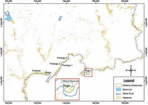
Figure 4. Floodplain wetland probability map of the White Volta Basin, Ghana. (Map was generated using seven variables as input into the logistic regression model). For full color versions of the figures in this paper, please see the online version.

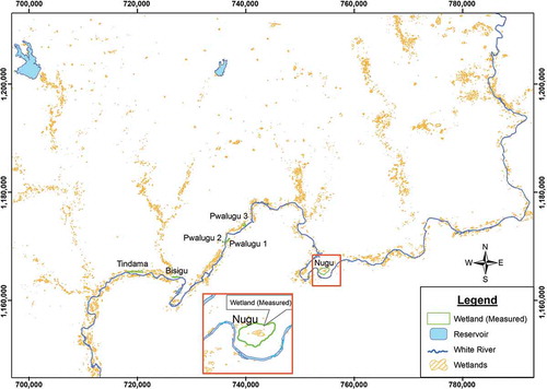
Table 8 indicates the reliability of the prediction obtained using seven explanatory variables and on the average, pixels classified were 98.48% in agreement with the modeled sites. The agreement between modeled wetland and classified wetland stands at 47%, while that between modeled non-wetland and classified non-wetland is about 99%. The high level of accuracy of the results presented was a reflection of the dominance of other features in the population other than the wetlands.

Table 8. Error matrices of classified and modeled wetland data using seven variables within the logistic regression.

Modeled	Classified		Total
	Wetland	No wetland
Overall accuracy = 98.48%
Kappa coefficient = 0.41
Wetland	50,579	85,263	135,842
No wetland	56,992	9,151,469	9,208,461
Total	107,571	9,236,732	9,344,303
Modeled	Prod. Acc. (Pixels)	User Acc. (Pixels)
Wetland	50,579/107,571	50,579/135,842
No wetland	9,151,469/9,236,732	9,151,469/9,208,461

Using the logistic regression model within the GIS platform, a total of 259.5 km² of the land area is estimated as wetland within the study area of 8410 km², as compared with 85.26 km² mapped using the maximum likelihood method. To give credence to the model, the empirical probabilities (Table 9) of selected modeled wetlands were estimated to determine if they occurred in the field. In relation to the modeled wetlands, the estimator probabilities calculated show that they closely related to the existing wetland in the fields.

Table 9. Empirical probabilities of modeled and measured floodplain wetlands.

Location	Modeled wetland (m^2)	Measured wetland (m^2)	P(E) =  (E/N)
Tindama	386,749.96	617,331.79	0.62
Bisigu	1213.65	150,562.82	0.01
Pwalugu 1	107,858.16	135,511.43	0.80
Pwalugu 2	25,973.77	32,332.21	0.80
Pwalugu 3	149,308.69	201,068.8	0.74
Nugu	104,828.95	156,692.23	0.70

Note: Empirical probability estimates probabilities from experience and observation. Empirical probability P(E) = modeled event (E)/measured event (N).

4. Discussion

The results of the logistic regression models used show that not all explanatory variables used had an influence on the location and distribution of floodplain wetlands. Variables such as slope, internal relief, wetness, and geology were considered insignificant. The significant variables such as distance, evapotranspiration, texture, logarithmic transformation of band 4 (wavelength λ of 0.77–0.90 µm), shape index, elevation, and SAVI were used to determine the occurrence or non-occurrence of wetlands. For instance, distance from the main river channel on either side of the bank had a negative relationship with wetland presence indicating that a change in distance of 0.7 km from the river course reduces the chance of encountering wetlands on the floodplain. In other words, the probability of encountering a wetland decreased with increasing distance from the river system, wetlands on the floodplain being fed seasonally by overbank flow and foot-slope recharge.

Evapotranspiration results from the processes of energy and water exchange between a wetland and its surroundings. Evapotranspiration of 0.37 mm/day during the rainy season (July to October) influenced the sustainability of wetlands indicating a low water extraction rate within the study sites. It is worth mentioning that water supply, heat conditions, humidity, intensity of air turbulence, and material composition of the underlying surface control evapotranspiration within the wetlands. Field observations during the period of October showed that crops in the field were harvested, thus exposing bareland. Hence, areas with high vegetation density and evapotranspiration have a high probability of being associated with a floodplain wetland.

The texture predictor showed a high probability of separating wetland pixels from non-wetland pixels. Texture gives information regarding contrast uniformity, rugosity, and regularity. Hence, a change in image roughness by 0.03% enhances the filter’s contribution to the classification of wetlands in the basin. The image predictor log B4, which is the logarithm transformation of the Landsat band 4 of October 2002, is powerful enough to discriminate between vegetation and water bodies. In areas with low vegetation density, log B4 has less power to discriminate between water bodies and vegetation. However, only a fraction of the landscape can be mapped. It is important to note that turbidity of water becomes an important factor in establishing a relationship between a wetland and its environs. The reflectance of water in wetlands changes with the amount of sediment, and increases in the concentration of sediment bring about changes in the reflectance of wetland pixels. These increases make it difficult to locate and delineate wetlands.

From the geomorphological perspective, the development of wetlands depends on the compactness and connectivity of the landscape. The shape index determines the compactness of the landscape. Areas on floodplains marked as wetland sites showed high levels of compactness and connectivity. This shape index agrees with the natural shape of most wetlands and is thus characterized by a small index. Additionally, elevation has a negative influence on floodplain wetlands, which traverse throughout the catchment. Wetlands were not found in the highlands because the configuration of the Gambaga Ranges does not support the stagnation of water. Wetlands have a dynamic environment, and they can experience natural fluctuations in water level. Consequently, plants found within a wetland are able to tolerate both flooding and short periods of drought within a year. During the early part of the dry season, as indicated on the image, the sparseness of vegetation shows a high level of radiative mixing of soils and plants where the leaf elements of a canopy are assumed to be opaque (Gilabert et al. 2002). As long as the canopies of plants are actively photosynthesizing, red extinction through a canopy will exceed that of the near-infrared, and a soil correction is necessary. The SAVI removes the soil background noise and makes it more linear with biophysical plant parameters. Hence, the use of SAVI in the modeling process minimizes soil brightness influence from spectral vegetation indices involving red and near-infrared wavelengths.

The magnitude of the influence of each explanatory variable is determined by examining its marginal effects. Marginal effect provides a good approximation of the amount of change in the probable location of a floodplain wetland that will be produced by a change of a unit in the explanatory variables in the equation (see Table 6). In this study, distance showed a higher influence on the location of wetlands on the floodplain. For instance, a small change in distance away from the main river course influences the model’s ability to locate wetlands. Floodplain wetlands are found along rivers and any departure from the river reduces the probability of locating floodplain wetlands. In the White Volta River Basin, higher evapotranspiration rates in the wetland landscape, as estimated by Compaore (2006), have a high propensity as a proxy to locate wetlands. Evapotranspiration used in the model indicated a lower marginal effect. The rate of evapotranspiration in wetlands varies over a range of space and timescales influenced by the relationship of the water table to the root zone and the timing of plant senescence. Such discrepancies illustrate potential problems with extrapolating off-site estimates of evapotranspiration or single measurements of evapotranspiration from a site over space or time.

5. Conclusion

Wetlands on the floodplain within the White Volta River Basin play an important role in the dry season agriculture and ecosystem management. However, researchers and basin managers have no knowledge about their number, surface area, nature (temporary and permanent), and distribution patterns. This paper explores the use of spatial extracted variables, logistic regression, and GIS to map out floodplain wetlands in the White Volta River Basin. From the results, we noticed that when logistic regression model and ancillary variables combined within the GIS platform, it was possible to determine factors that can assist in delineating or distinguishing probable wetland sites from the surrounding landscape. The logistic regression model produced significant coefficient and model statistics for assessing the accuracy of the derived function and the role that predicted parameters played in wetland mapping. Insignificant parameters were eliminated using VIF and multicollinearity and parameters that showed little multicollinearity were incorporated into the model. The model used was about 98.48% accurate in predicting wetland presence. The high accuracy of 98.48% was achieved by using a combination of methods; these included field visits, high-resolution image interpretation, and statistical analysis.

During the processes of conceptualization, data collection, analysis within the geospatial platform, and interpretation, the researchers observed some uncertainties in the results. These uncertainties were caused by errors in DEM, and errors that occurred during the process of deriving some of the explanatory variables such as shape, texture, height, and log B4. Aside from these uncertainties, the processes adopted to map out floodplain wetlands performed well and areas with wetlands were assigned high probability.

The results from the study demonstrate that the logistic regression model operationalized in the GIS platform provides an improved method for mapping and updating wetland conditions in Ghana. Wetland maps of this spatial resolution would enable calculations of wetland areas, as well as enabling rapid change-detection methods.

The results provided further evidence that highly accurate detection of wetland cover is feasible using semiautomated classification procedures. This study revealed that basic statistical and spatial techniques could be used as a tool to acquire ecologically relevant information on temporary and permanent floodplain wetlands that are larger than the resolution of images used for classification. In this case, mapping of floodplain wetland characteristics could provide important information for ecological research and development of conservation measures. This research corroborates the findings of a study by Baker et al. (2006) that applying a multiplicity of techniques can improve mapping accuracy. Additionally, the outcomes of the research complements other forms of work (Li, Im, and Beier 2013; Lersch and Haertel 2010) that show that the use of ancillary data could help improve the mapping of spatial features or occurrences. As a follow-up to this research, there is a need to identify additional relevant ancillary data as an input into the logistic regression model that would be used to extract wetlands at a higher accuracy level. Applying the logistic regression method in this work was time-consuming and laborious. However, researchers are encouraged to investigate further the ability of logistic regression techniques to be incorporated or developed as a routine that can classify specific wetland types and also to verify the potential of using a combination of data from higher resolution sensors and radar images with a routine process.

Disclosure statement

No potential conflict of interest was reported by the authors.

Acknowledgements

The authors are grateful to the many field assistants who helped with the collection of data.

ORCID

Benjamin K. Nyarko http://orcid.org/0000-0002-6560-9613

Nick C. Van De Giesen http://orcid.org/0000-0002-7200-3353

Additional information

Funding

The work presented is part of the PhD research work of the first author, which was funded by the German Ministry of Education and Research (BMBF), the GLOWA-Volta Project, and the Centre for Development Research (ZEF), Germany.

References

- Aguirre-Salado, C. A., E. J. Treviño-Garza, O. A. Aguirre-Calderón, J. Jiménez-Pérez, M. A. González-Tagle, L. Miranda-Aragón, J. R. Valdez-Lazalde, A. I. Aguirre-Salado, and G. Sánchez-Díaz. 2012. “Forest Cover Mapping in North-Central Mexico: A Comparison of Digital Image Processing Methods.” GIScience & Remote Sensing 49: 6.
- Anys, H., A. Bannari, D. C. He, and D. Morin. 1994. “Texture Analysis for the Mapping of Urban Areas Using Airborne MEIS-II Images.” In Proceedings of the First International Airborne Remote Sensing Conference and Exhibition, Vol. 3, Strasbourg, September 12–15, 231–245. Ann Arbor: Environmental Research Institute of Michigan.
- Arnold, N. 2010. “A New Approach for Dealing with Depressions in Digital Elevation Models When Calculating Flow Accumulation Values.” Progress in Physical Geography 34: 781.
- ASTER Validation Team. 2009. “ASTER Global DEM Validation Summary Report.” ASTER GDEM Validation Team: METI, NASA and USGS in cooperation with NGA and other collaborators. Accessed January 20, 2013. http://www.terrainmap.com/downloads/ASTER_GDEM_Validation_Summary_Report_FINAL_for_Posting_06-28-09%5B1%5D.pdf
- Baker, C., R. Lawrence, C. Montagne, and D. Patten. 2006. “Mapping Wetlands and Riparian Areas Using Landsat ETM+ Imagery and Decision-Tree-Based Models.” Wetlands 26: 465–474. doi:10.1672/0277-5212(2006)26[465:MWARAU]2.0.CO;2.
- Bastiaanssen, W. G. M., H. Pelgrum, J. Wang, Y. Ma, J. Moreno, G. J. Roerink, and T. Van Der Wal. 1998b. “A Remote Sensing Surface Energy Balance Algorithm for Land (SEBAL).” Journal of Hydrology 212–213: 213–229. doi:10.1016/S0022-1694(98)00254-6.
- Beven, K. J., and M. J. Kirkby. 1993. Channel Network Hydrology. Chichester: Wiley & Sons.
- Cahill, L. W., and G. Deng. 1997. “An Overview of Logarithm-Based Image Processing Techniques for Biomedical Applications.” In 13th International Conference on Digital Signal Processing Proceedings, Vol. 1, July 2–4, 93–96. Patras: TYPORAMA.
- Chen, C., C. Chen, and N.-T. Son. 2012. “Investigating Rice Cropping Practices and Growing Areas from MODIS Data Using Empirical Mode Decomposition and Support Vector Machines.” GIScience & Remote Sensing 49: 117–138. doi:10.2747/1548-1603.49.1.117.
- Chengmin, H., and J. Lynn. 2008. “Multi-Criteria Wetlands Mapping Using an Integrated Pixel-Based and Object-Based Classification Approach.” Colorado Department of Transportation Dtd Applied Research and Innovation Branch, Report No. Cdot-2008-8.
- Compaore, H. 2006. “The Impact of Savannah Vegetation on the Spatial and Temporal Variation of the Actual Evapotranspiration in the Volta Basin, Navrongo, Upper East Ghana.” Ecology and Development Series, No. 36. Gottingen: Cuvillier Verlag.
- De Alwis, D. A., Z. M. Easton, H. E. Dahlke, W. D. Philpot, and T. S. Steenhuis. 2007. “Unsupervised Classification of Saturated Areas Using a Time Series of Remotely Sensed Images.” Hydrology and Earth System Sciences 11: 1609–1620. doi:10.5194/hess-11-1609-2007.
- De Roeck, E. R., N. E. C. Verhoest, M. H. Miya, H. Lievens, O. Batelaan, A. Thomas, and L. Brendonck. 2008. “Remote Sensing and Wetland Ecology: A South African Case Study.” Sensors 8 (5): 3542–3556. doi:10.3390/s8053542.
- Debella-Gilo, M., and B. Etzelmüller. 2009. “Spatial Prediction of Soil Classes Using Digital Terrain Analysis and Multinomial Logistic Regression Modeling Integrated in GIS: Examples from Vestfold County, Norway.” Catena 77: 8–18. doi:10.1016/j.catena.2008.12.001.
- Dekok, R., T. Schneider, M. Baatz, and U. Ammer. 1999. “Object Based Image Analysis of High Resolution Data in the Alpine Forest Area.” In Joint WS ISPRS WG I/1, I/3 and IV/4: Sensors and Mapping from Space 1999, Hannover, September 27–30. Lemmers: GITC BV.
- Dewey, J. C., S. H. Schoenholtz, J. P. Shepard, and M. G. Messina. 2006. “Issues Related to Wetland Delineation of a Texas, USA Bottomland Hardwood Forest.” Wetlands 26: 410–429. doi:10.1672/0277-5212(2006)26[410:IRTWDO]2.0.CO;2.
- Dong, Y., G. Tang, and T. Zhang, 2008. “A Systematic Classification Research of Topographic Descriptive Attribute in Digital Terrain Analysis.” In The International Archives of the Photogrammetry, Remote Sensing and Spatial Information Sciences, Vol. Xxxvii, Part B2, Beijing. Lemmers: GITC BV.
- Duadze, S. E. K. 2004. “Land Use and Land Cover Study of the Savannah Ecosystem in the Upper West Region (Ghana) Using Remote Sensing.” In Ecology and Development Series, No. 16. Gottingen: Cuvillier Verlag.
- Dwivedi, R., B. Rao, and S. Bhattacharya. 1999. “Mapping Wetlands of the Sundaban Delta and its Environs Using Ers-1 Sar Data.” International Journal of Remote Sensing 20: 2235–2247. doi:10.1080/014311699212227.
- Fisher, R. B. 1999. “Special Cases Where Benefits Arise From Using the Logarithm Transform for Illumination Invariant Feature Extraction.” Accessed May 4, 2009. http://Homepages.Inf.Ed.Ac.Uk/Rbf/Papers/ Constant.Pdf
- Gilabert, M. A., J. González-Piqueras, F. J. Garcı́a-Haro, and J. Meliá. 2002. “A Generalized Soil-Adjusted Vegetation Index.” Remote Sensing of Environment 82: 303–310. doi:10.1016/S0034-4257(02)00048-2.
- Grabs, T., J. Seibert, K. Bishop, and H. Laudon. 2009. “Modeling Spatial Patterns of Saturated Areas: A Comparison of the Topographic Wetness Index and a Dynamic Distributed Model.” Journal of Hydrology 373 (1–2): 15–23. doi:10.1016/j.jhydrol.2009.03.031.
- Guneralp, I., A. M. Filippi, and B. U. Hales. 2013. “River-Flow Boundary Delineation from Digital Aerial Photography and Ancillary Images Using Support Vector Machines.” GIScience and Remote Sensing 51: 1–25.
- Harvey, K. R., and G. J. E. Hill. 2001. “Vegetation Mapping of a Tropical Freshwater Swamp in the Northern Territory, Australia: A Comparison of Aerial Photography, Landsat TM and Spot Satellite Imagery.” International Journal of Remote Sensing 22: 2911–2925. doi:10.1080/01431160119174.
- Heinl, M., J. Walde, G. Tappeiner, and U. Tappeiner. 2009. “Classifiers Vs. Input Variables – The Drivers in Image Classification for Landcover Mapping.” International Journal of Applied Earth Observation and Geoinformation 11: 423–430. doi:10.1016/j.jag.2009.08.002.
- Hengl, T., S. Gruber, and D. P. Shrestha. 2003. Terrain Analysis in ILWIS: Lecture Notes and User Guide. Enschede: ITC.
- Islam, Md, A., P. S. Thenkabail, R. W. Kulawardhana, R. Alankara, S. Gunasinghe, C. Edussriya, and A. Gunawardana. 2008. “Semi-Automated Methods for Mapping Wetlands Using Landsat ETM+ and SRTM Data.” International Journal of Remote Sensing 29 (24): 7077–7106. doi:10.1080/01431160802235878.
- Jain, S. K., R. D. Singh, M. K. Jain, and A. K. Lohani. 2005. “Delineation of Flood-Prone Areas Using Remote Sensing Techniques.” Water Resources Management 19: 333–347. doi:10.1007/s11269-005-3281-5.
- Jensen, J. R., M. E. Hodgson, M. Garcia-Quijano, J. Im, and J. A. Tullis. 2009. “A Remote Sensing and GIS-Assisted Spatial Decision Support System for Hazardous Waste Site Monitoring.” Photogrammetric Engineering & Remote Sensing 75 (2): 169–177. doi:10.14358/PERS.75.2.169.
- Kesse, G. O. 1985. The Mineral And Rock Resources Of Ghana. Rotterdam: Balkema.
- Knight, A. W., D. R. Tindall, and B. A. Wilson. 2009. “A Multitemporal Multiple Density Slice Method for Wetland Mapping Across the State of Queensland, Australia.” International Journal of Remote Sensing 30 (13): 3365–3392. doi:10.1080/01431160802562180.
- Krishnapuram, B., L. Carin, M. A. T. Figueiredo, and A. J. Hartemink. 2005. “Sparse Multinomial Logistic Regression: Fast Algorithms and Generalization Bounds.” IEEE Transactions on Pattern Analysis and Machine Intelligence 27 (6): 957–968. doi:10.1109/TPAMI.2005.127.
- Kumar, L., and P. Sinha. 2014. “Mapping Salt-Marsh Land-Cover Vegetation Using High-Spatial and Hyperspectral Satellite Data to Assist Wetland Inventory.” GIScience and Remote Sensing 51: 483–497. doi:10.1080/15481603.2014.947838.
- Lersch, R., and V. Haertel. 2010. “On the Use of Ancillary Data by Applying the Concepts of the Theory of Evidence to Remote Sensing Digital Image Classification.” International Journal of Remote Sensing 31 (12): 3211–3221. doi:10.1080/01431160903159324.
- Lersch, R., V. Haertel, and Y. R. Shimabukuro. 2007. “On the Use of Ancillary Data by Applying the Concepts of the Theory of Evidence to Remote Sensing Digital Image Classification.” In Geoscience and Remote Sensing Symposium, IGARSS 2007 in IEEE International, 2063–2066. Barcelona: IEEE.
- Li, M., J. Im, and C. Beier. 2013. “Machine Learning Approaches for Forest Classification and Change Analysis Using Multi-Temporal Landsat TM Images over Huntington Wildlife Forest.” GIScience and Remote Sensing 50: 361–384.
- Liames, J. S., R. G. Congalton, and R. S. Lunetta. 2013. “Analyst Variation Associated with Land Cover Image Classification of Landsat ETM + Data for the Assessment of Coarse Spatial Resolution Regional/Global Land Cover Products.” GIScience & Remote Sensing 50 (6): 604–622.
- Lillesand, T. M., R. W. Kiefer, and J. Chipman. 2008. Remote Sensing and Image Interpretation. New York: John Wiley & Sons.
- Lindsay, J. B., and M. G. Evans. 2008. “The Influence of Elevation Error on the Morphometrics of Channel Networks Extracted from DEMs and the Implications for Hydrological Modelling.” Hydrological Processes 22: 1588–1603. doi:10.1002/hyp.6728.
- MacLean, M. G., and R. G. Congalton. 2011. “Investigating Issues in Map Accuracy When Using an Object Based Approach to Map Benthic Habitats.” GIScience & Remote Sensing 48 (4): 457–477. doi:10.2747/1548-1603.48.4.457.
- Mahmood, S. A., and R. Gloaguen. 2011. “Analyzing Spatial Autocorrelation for the Hypsometric Integral to Discriminate Neotectonics and Lithologies Using DEMs and GIS.” GIScience & Remote Sensing 48 (4): 541–565. doi:10.2747/1548-1603.48.4.541.
- Mallinis, G., and N. Koutsias. 2008. “Spectral and Spatial-Based Classification for Broad-Scale Land Cover Mapping Based on Logistic Regression.” Sensors 8: 8067–8085. doi:10.3390/s8128067.
- May, D., J. Wang, J. Kovacs, and M. Muter. 2002. Mapping Wetland Extent Using Ikonos Satellite Imagery of the O’Donnell Point Region, Georgian Bay, Ontario. London: Department of Geography, University of Western Ontario.
- Meijerink, A. M. J. 2002. “Satellite Eco-Hydrology – A Review.” Tropical Ecology 43: 91–106.
- Menard, S., ed. 1995. “Applied Logistic Regression Analysis.” In Sage University Paper Series on Quantitative Applications in the Social Sciences, 7–106. Thousand Oaks, CA: Sage.
- Merot, Ph., H. Squividant, P. Aurousseau, M. Hefting, T. Burt, V. Maitre, et al. 2003. “Testing a Climato-Topographic Index for Predicting Wetlands Distribution Along a European Climate Gradient.” Ecological Modelling 163 (1–2): 51–71. doi:10.1016/S0304-3800(02)00387-3.
- Mitsch, W. J., and J. G. Gosselink. 2000. “The Value of Wetlands: Importance of Scale and Landscape Setting.” Ecological Economics 35: 25–33. doi:10.1016/S0921-8009(00)00165-8.
- Mladinich, C. S. 2010. “An Evaluation of Object-Oriented Image Analysis Techniques to Identify Motorized Vehicle Effects in Semi-arid to Arid Ecosystems of the American West.” GIScience & Remote Sensing 47 (1): 53–77. doi:10.2747/1548-1603.47.1.53.
- Moore, I. D. 1996. “Hydrologic Modeling and GIS.” In GIS and Environmental Modeling: Progress and Research Issues, edited by M. F. Goodchild, L. T. Steyaert, B. O. Parks, C. Johnston, D. Maidment, M. Crane, and S. Glendinning, 143–148. Fort Collins, CO: GIS World Books.
- Nielsen, E. M., S. D. Prince, and G. T. Koeln. 2008. “Wetland Change Mapping for the U.S. Mid-Atlantic Region Using an Outlier Detection Technique.” Remote Sensing of Environment 112: 4061–4074. doi:10.1016/j.rse.2008.04.017.
- Nyarko, B. K.. 2007. “Floodplain Wetland Riverflow Synergy in the White Volta River Basin, Ghana.” Ecology and Development Series, Bd. No. 53.
- Ozesmi, S. L., and M. E. Bauer. 2002. “Satellite Remote Sensing of Wetlands.” Wetlands Ecology and Management 10: 381–402. doi:10.1023/A:1020908432489.
- Panda, S. K., A. Prakash, M. T. Jorgenson, and D. N. Solie. 2012. “Near-Surface Permafrost Distribution Mapping Using Logistic Regression and Remote Sensing in Interior Alaska.” GIScience & Remote Sensing 49: 346–363. doi:10.2747/1548-1603.49.3.346.
- Pantaleoni, E., R. H. Wynne, J. M. Galbraith, and J. B. Campbell. 2009. “A Logit Model for Predicting Wetland Location Using ASTER and GIS.” International Journal of Remote Sensing 30 (9): 2215–2236. doi:10.1080/01431160802549310.
- Phillips, J. D. 1990. “A Saturation-Based Model of Relative Wetness for Wetland Identification.” Journal of the American Water Resources Association 26 (2): 333–342. doi:10.1111/j.1752-1688.1990.tb01376.x.
- Pooja, A. P., J. Jayanth, and K. Shivaprakash. 2011. “Classification of RS Data Using Decision Tree Approach.” International Journal of Computer Applications 23 (3): 0975–8887.
- Pope, K., J. Rey-Benayas, and J. Paris. 1994. “Radar Remote Sensing of Forest and Wetland Ecosystems in the Central American Tropics.” Remote Sensing of Environment 48: 205–219. doi:10.1016/0034-4257(94)90142-2.
- Qi, P., C. Zhao, and Z. Feng. 2010. “GIS- and Machine Learning-Based Modeling of the Potential Distribution of Broadleaved Deciduous Forest in the Chinese Loess Plateau.” GIScience & Remote Sensing 47: 99–114. doi:10.2747/1548-1603.47.1.99.
- Ramsar. 2004. The Ramsar Convention Manual: A Guide to the Convention on Wetlands (Ramsar, Iran, 1971). 3rd ed. Gland: Ramsar Convention Secretariat. http://www.Ramsar.Org/Lib/Lib_Manual2004e.Htm.
- Ricchetti, E. 2000. “Multispectral Satellite Image and Ancillary Data Integration for Geological Classification.” Photogrammetric Engineering and Remote Sensing 66 (4): 429–435.
- Richards, J. A. 1999. Remote Sensing Digital Image Analysis. Berlin: Springer-Verlag.
- Rogan, J., J. Franklin, D. Stow, J. Miller, C. Woodcock, and D. Roberts. 2008. “Mapping Land-Cover Modifications over Large Areas: A Comparison of Machine Learning Algorithms.” Remote Sensing of Environment 112: 2272–2283. doi:10.1016/j.rse.2007.10.004.
- Shaikh, M., D. Green, and H. Cross. 2001. “A Remote Sensing Approach to Determine Environmental Flows for Wetlands of the Lower Darling River, New South Wales, Australia.” International Journal of Remote Sensing 22: 1737–1751. doi:10.1080/01431160118063.
- Stoler, J., D. Daniels, J. R. Weeks, D. A. Stow, L. L. Coulter, and B. K. Finch. 2012. “Assessing the Utility of Satellite Imagery with Differing Spatial Resolutions for Deriving Proxy Measures of Slum Presence in Accra, Ghana.” GIScience & Remote Sensing 49 (1): 31–52. doi:10.2747/1548-1603.49.1.31.
- Su, L., and Y. Huang. 2009. “Support Vector Machine (SVM) Classification: Comparison of Linkage Techniques Using a Clustering-Based Method for Training Data Selection Issue.” GIScience & Remote Sensing 46 (4): 411–423. doi:10.2747/1548-1603.46.4.411.
- Sugumaran, R., J. Harken, and J. Gerjevic. 2004. “Using Remote Sensing Data to Study Wetland Dynamics in Iowa.” Iowa Space Grant (Seed) Final Technical Report, January.
- Sulebak, J. R., L. M. Tallaksen, and B. Erichsen. 2000. “Estimation of Areal Soil Moisture by Use of Terrain Data, Geografiska Annaler.” Series A, Physical Geography 82 (1): 89–105.
- Summers, P., C. S. Albert, J. Chung, and N. Alison. 2000. “Impact of Image Processing Operations on MR Noise Distributions.” In International Society for Magnetic Resonance in Medicine, The 8th Scientific Meeting and Exhibition, Denver, CO, April 3–7, 1779. Berkeley, CA: ISMRM.
- Tenenbaum, D. E., Y. Yang, and W. Zhou. 2011. “A Comparison of Object-Oriented Image Classification and Transect Sampling Methods for Obtaining Land Cover Information from Digital Orthophotography.” GIScience & Remote Sensing 48 (1): 112–129. doi:10.2747/1548-1603.48.1.112.
- Van De Giesen, N. 2001. “Characterization of West African Shallow Flood Plains With L- And C-Band Radar.” IAHS Publication 267: Remote Sensing and Hydrology, 2000, 365–367. IAHS Press.
- Wakeley, J. S., S. W. Sprecher, and R. W. Lichvar. 1996. “Relationships Among Wetland Indicators in Hawaiian Rain Forest.” Wetlands 16: 173–184. doi:10.1007/BF03160691.
- Wilson, J. P., C. S. Lam, and Y. Deng. 2007. “Comparison of the Performance of Flow-Routing Algorithms Used in GIS-Based Hydrologic Analysis.” Hydrological Processes 21: 1026–1044. doi:10.1002/hyp.6277.
- Wright, C., and A. Gallant. 2007. “Improved Wetland Remote Sensing in Yellowstone National Park Using Classification Trees to Combine TM Imagery and Ancillary Environmental Data.” Remote Sensing of Environment 107 (4): 582–605. doi:10.1016/j.rse.2006.10.019.
- Zhang, C., Z. Xie, and D. Selch. 2013. “Fusing Lidar and Digital Aerial Photography for Object-Based Forest Mapping in the Florida Everglades.” GIScience and Remote Sensing 50: 562–573.
- Zhang, D., C. Zhang, R. Cromley, D. Travis, and D. Civco. 2012. “An Object-Based Method for Contrail Detection in AVHRR Satellite Images.” GIScience & Remote Sensing 49: 412–427. doi:10.2747/1548-1603.49.3.412.
- Zhu, L., and J.-F. Huang. 2006. “GIS-Based Logistic Regression Method for Landslide Susceptibility Mapping in Regional Scale.” Journal of Zhejiang University Science A 7: 2007–2017. doi:10.1631/jzus.2006.A2007.