Mapping land development through periods of economic bubble and bust in Massachusetts using Landsat time series data

Abstract

This study examines the change from undeveloped to developed land-use during the real estate bubble (2000–2006) and subsequent bust (2006–2013) in Massachusetts, USA, using a time series of Landsat-5, 7, and 8 data. Loss in undeveloped land-use was measured using standardized change detection of Landsat green vegetation and albedo fractions. Between periods of bubble and bust, a significant difference occurred in the total area of undeveloped land-use loss (bubble, 35.9 km²; bust, 29.18 km²), as well as mean loss-patch area (p < 0.001), from 4848 m² to 4079 m² (16% decrease). The area of undeveloped land-use loss was 81% greater in forest than agricultural land-use during the bubble and only 51% greater, post-bubble. Undeveloped urban forest loss constituted 25% of all losses during the bubble, while during the bust it was 42%. These findings indicate that total area of undeveloped land-use loss changed due to the economic recession and that those losses reorient from forest and agricultural areas toward areas adjacent to existing development (i.e., urban forests).

Keywords:

• land-use change
• economic recession
• Landsat
• spectral mixture analysis
• Massachusetts

Introduction

Since World War II, the area of residential land-use in the United States has approximately tripled while the population has only doubled, and urban land-use is projected to increase by over 75% in the next 40 years (Radeloff et al. 2012; Mockrin et al. 2013). In most scenarios, residential land development increases the density of housing and roads, displacing species and fragmenting wildlife habitats and corridors within 50 km (Radeloff et al. 2005; Slonecker, Milheim, and Claggett 2010; Gagné and Fahrig 2011). The ecological impact of encroaching residential land-use near protected land constitutes a major threat to their intended purpose of preserving natural space and biodiversity (Radeloff et al. 2010). Additionally, increased presence of exotic and invasive species is linked to residential land-use (Gavier-Pizarro et al. 2010), costing roughly $120 billion a year for mitigation efforts (Pimentel, Zuniga, and Morrison 2005; Dodds and Orwig 2011). Regional policy decisions about land-use conversion, and thereby its ecological impact, are often coupled with perceptions of current and future economic conditions (Radeloff et al. 2012). This study investigates the impact of the recent housing boom period (2000–2006) versus bust period (2006–2013) on loss of agricultural and forest land-use to residential and commercial development in Massachusetts, USA.

The 2000–2006 housing bubble

The period from 2000 to 2006 represents the time span of the most recent housing “bubble” in the United States (Baker 2005; Dokko et al. 2011; Bluestone et al. 2012; Levitin and Wachter 2012; Fitzgerald 2013). Low interest rates set by the US Federal Reserve and pervasive mortgage loans by banks drove unprecedented demand for new homes in the late 1900s through 2006. (Dokko et al. 2011; Glaeser, Gottleb, and Gyourko 2010). On average, residential investment as a percent of GDP has exceeded nonresidential investment by a factor of 1.4 since the 1950s and has been considerably more volatile (Figure 1). Between 1974 and 2001, residential investment averaged 4.5% of the US GDP, and by 2005 it reached 6.6% – the highest it had been since 1950. The housing bubble burst through 2006–2007, when mortgage defaults began to rapidly rise and banks stopped providing the risky loans that drove inflated demand for homes during the bubble (Glaeser, Gottleb, and Gyourko 2010; Levitin and Wachter 2012). By 2010, residential investment fell to 2.4% of GDP – the lowest in 60 years (US Department of Commerce 2014).

Figure 1. Real estate investment as percent of US GDP from 1947 to 2013. The second highest point of residential investment is in 2005, while the lowest is in 2010 (US Department of Commerce 2014).

During the bubble, resources and labor for residential construction were siphoned from the commercial sector in order to meet the increased demand for new homes (Mulligan 2010). Investment in nonresidential real estate reached its lowest point in over 50 years (2.4% of GDP) during the bubble, while in 2008, after the bubble burst, it increased 12% above the previous 60-year average (3.8% of GDP; US Department of Commerce 2014). Before the 2006 housing bust, Massachusetts issued an average of 17,849 new housing permits annually (1995–2000), 24,549 at the peak of the bubble in 2005, and 7941 in 2009 post-bubble (Figure 2; US Census Bureau 2014). From 1999 to 2005, residential development accounted for 87% of land-use change in the state (DeNormandie and Corcoran 2009). Before, throughout, and after the recent housing bubble, demand for new homes in Massachusetts has consistently outpaced supply, and is likely to continue into the foreseeable future (Fitzgerald 2013).

Figure 2. Authorized new housing units in Massachusetts from 1995 to 2013 (US Census Bureau 2014).

Land-use change in Massachusetts

The impact of the most recent economic recession on land-use conversion is currently unknown throughout the United States, and has particular relevance in the New England Region, where agricultural abandonment to forest transition has been reversed in many locations recently due to over 60 km² per year (2000–2005; excluding Maine) of urban development (Jeon, Olofsson, and Woodcock 2014). Massachusetts was predominantly old-growth forest before the seventeenth century, and then transformed to agricultural land by the mid-nineteenth century (Foster et al. 2005). The state transitioned to secondary forest by the mid-twentieth century with migration to industrial centers and more profitable farmlands in states west of New England (2005; Jeon, Olofsson, and Woodcock 2014). An extensive network of highways and commuter rails developed around the Greater Boston area from the 1950s onward, supported suburbanization and the shift from an industrial economy to a knowledge-based economy (McCauley et al. 2015).

At the onset of the recent housing bubble, approximately 57% of Massachusetts was forested and it had the third highest population density in the United States. At this time in Massachusetts, new land development for residential or commercial real estate would typically result in loss of forest or agricultural land at a ratio of 3:1 (DeNormandie and Corcoran 2009; Jeon, Olofsson, and Woodcock 2014). Beyond the typical woodland forest vulnerability to land conversion, urban forests in Massachusetts, comprised of backyard trees, municipal parks, and street trees, urban woodlots and shrub-grasslands are also subject to loss through land development (Hostetler et al. 2013). Agricultural land-use in Massachusetts is especially vulnerable to conversion, because it can be developed with relative ease, compared to forested land (DeNormandie and Corcoran 2009; Slonecker, Milheim, and Claggett 2010). The arrangement of forest, woodland, and agricultural land-uses is defined in this study as “undeveloped land-use” (Rogan and Chen 2004). Undeveloped land-use provides a variety of benefits, such as carbon sequestration, pollution mitigation, erosion and runoff control, and evaporative cooling (Foster et al. 2005; Nowak, Wang, and Endreny 2007; Václavík and Rogan 2009; Abdullahi et al. 2015), rendering Massachusetts $6 billion worth of ecosystem services per year (DeNormandie and Corcoran 2009).

Monitoring changes in forest and undeveloped land-use is critical to producing, implementing, and assessing land-use and land protection policies (Foster et al. 2005; Aber et al. 2010; Slonecker, Milheim, and Claggett 2010). Literature exists on the history of land-use change in Massachusetts including the bubble (Foster et al. 2005; DeNormandie and Corcoran 2009; Jeon, Olofsson, and Woodcock 2014; McCauley et al. 2015); however, none have examined the latest period of economic bust.

This paper investigates whether growth in land development significantly changed during economic recession, using a case study in Massachusetts, USA. The area and pattern of undeveloped land-use converted in central Massachusetts during the most recent housing bubble (2000–2006) will be compared to after the bubble burst (2006–2013). Undeveloped land-use loss was measured using standardized change detection of vegetation and albedo fraction images generated using spectral mixture analysis.

Study area

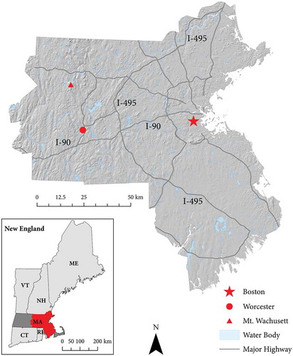
The study area (Figure 3) consists of the eastern and central portions of Massachusetts (USA), covering 11,711 km² (43% of the State) and encompassing 224 of the 351 towns in the state, including the Greater Boston metropolitan area as well as Worcester – the second largest city in New England. The population of the study area was 5,466,797, which was 83% of the state’s total population in 2010, and had a growth rate of 0.48% over the previous 20 years (US Census Bureau 2010). The landscape consists of dense urban land-use in the east surrounding Boston, suburban in the central portion, and predominantly forest in the west. Forests hold a diverse range of primarily hardwood species followed by conifer, and are defined along a spectrum from urban forests that include residential, park, and street trees to contiguous suburban and rural woodlands (Foster et al. 2005). Undeveloped land-use in the study area is comprised of mixed agriculture, hardwood, conifer, and mixed forest (53% of study area; MaFoMP 2011), while developed land-use is mostly low- to high-density residential and commercial (24% of study area). Agricultural land-use (9% of study area) is made up of over 4000 farms, which are primarily family-owned and -operated (>80%), producing mainly nursery products and fruits and vegetables (Massachusetts Department of Agricultural Resources 2014). An extensive transportation network of highways and commuter rails, including Interstate-495 running north–south and Interstate-90 running east–west through the study area, support multiple commercial centers and bedroom communities within the Greater Boston area (McCauley et al. 2015).

Figure 3. Study area of central Massachusetts, USA, with major cities, highways (including Interstate-495 and 90), Wachusett Mountain, and water bodies.

Data

Landsat data

The data used in land-use change analysis are listed in Table 1. Six level-1T Landsat-7 Enhanced Thematic Mapper-Plus (ETM+) (27 September 2000), Landsat-5 Thematic Mapper (TM) (20 September 2006), and Landsat-8 Operational Land Imager (OLI) (23 September 2013) images (path 12, row 30, and path 12, row 31) were used to detect/map land-use change. The Landsat images were selected to represent the onset, peak, and current conditions of the study area in relation to the most recent housing bubble, and to achieve minimal cloud-cover and phenological consistency. Images for each date were mosaicked and masked to the study area. Atmospheric contamination was removed following conversion to at-sensor reflectance using the COS(T) method developed by Chavez (1996). Level 1T Landsat images were geometrically corrected prior to delivery and qualitatively assessed in a geographic information system (GIS), and determined to require no further geometric correction (Giner and Rogan 2012).

Table 1. Data used in this study.

Data	Resolution	Range	Units	Source
ETM+ Bands 1–5, 7: 27 September 2000	30 m	0–1	Ρ	USGS: http://glovis.usgs.gov/
TM Bands 1–5, 7: 20 September 2006	30 m	0–1	Ρ	USGS: http://glovis.usgs.gov/
OLI Bands 2–7: 23 September 2013	30 m	0–1	Ρ	USGS: http://glovis.usgs.gov/
Massachusetts land-use map: 2000 and 2009	30 m	16 land-use categories	n/a	Clark University *HERO Program

Note: *http://www.clarku.edu/departments/hero/

Land-use maps

Preexisting 30 m land-use maps (90% overall accuracy) representing land characteristics in 2000 and 2009 (MaFoMP 2011) were used to stratify the study area by three dominant land-use strata to calibrate the change detection and thresholding process, following an approach presented by Schwert et al. (2013): forest (orchard, hardwood, conifer, and mixed forest), urban forest (low- and high-density residential and commercial), and low vegetation (pasture/row crop, golf course, and grassland).

Google Earth^TM data

Google Earth^TM software is an interactive digital mosaic of current and historic aerial and satellite imagery at varying spatial resolutions covering most of the world (Google Inc 2014). Time series of high-resolution images in Google Earth^TM can be used for validation of change detection on coarser spatial resolution data, such as Landsat (Dorais and Cardille 2011). High spatial resolution imagery of the study area in Google Earth^TM from March 1995, December 2001, August 2003, September 2006, September 2010, and August 2013 was utilized to facilitate change detection and perform accuracy assessment.

Methods

All Landsat images were enhanced using spectral mixture analysis. Standardized change detection was performed to map biophysically significant patches of undeveloped land-use loss. Change detection was validated using high-resolution imagery and preexisting land-use maps.

Image enhancement

The preprocessed Landsat images were enhanced using spectral mixture analysis (SMA). SMA can mitigate the problem of mixed pixels often associated with low- to medium-resolution applications (Adams et al. 1995; Small 2001; Weng 2012). SMA produces sub-pixel proportions of endmembers, based on the linear correlation between user-defined vectors in feature space that are intended to represent the pure spectra of surface features of interest (Settle and Drake 1993).

Three endmembers were created for this analysis: (1) green vegetation; (2) high-albedo non-vegetation (developed/non-vegetation); and (3) low-albedo non-vegetation/shade (developed/non-vegetation) (Small 2001). A threshold of greater than 50% green vegetation was used to detect undeveloped land-use. Developed land-use has been characterized previously as locations with greater than 50% anthropogenic land-use (Schneider 2012). The intermixed wildland–urban interface is a common articulation point between humans and nature, and it has been parameterized as census blocks with greater than 50% undeveloped land-use and greater than 6.17 housing units/km² (Radeloff et al. 2005). Using a threshold of greater than 50% vegetation cover was additionally supported empirically through comparison of vegetation endmember fraction images to high-resolution imagery of the study area in Google Earth^TM by showing that these locations are dominated by vegetation cover. Visual inspection found that undeveloped surfaces typically had a high-albedo non-vegetation fraction of less than 10%; therefore, change detection was limited to only those pixels that were greater than 10% high-albedo non-vegetation fraction in the later year of each detection period. The low-albedo non-vegetation/shade endmember was not used in this study, because there was no difference that was empirically discernible between its values within undeveloped and developed land-uses.

The spectral profiles of five sets of image endmembers were produced and compared to reference spectral signatures of relevant materials from the Advanced Spaceborne Thermal Emission and Reflection Radiometer (ASTER) Spectral Library (Baldridge et al. 2009) to select the best set of three endmembers for SMA (Figure 4). SMA model error was quantified using root mean squared error (RMSE), with an average 0.031 units of proportional reflectance (0–1) for all three image dates. Locations of high RMSE (>2 standard deviations) were examined with fine spatial resolution imagery in Google Earth^TM and were found to be surface materials insufficiently represented by the suite of endmembers (e.g., wetland vegetation, bright bare soil, and grass).

Figure 4. Five endmember sets evaluated for use in spectral mixture analysis. The X-axis is the spectral range of Landsat-5 TM bands 1–5 and 7 (gray bars), and the Y-axis is mean proportional reflectance for each endmember in the set. Reflectance values were extracted from the 20 September 2006 Landsat-5 TM image. This figure was adapted from figure 3 in Small (2001).

Change detection

Change between green vegetation fraction images for each time period was mapped through a method of image differencing that normalizes deviations in phenological and solar conditions between Landsat capture dates developed by Rogan et al. (2013). Fraction images were converted to z-score and then used to derive proportional change (PC) according to:

(1)

PC_x is the proportional change of the endmember images used. Z_x is per-pixel z-score, StDev_x is the fractional image standard deviation, and _Ti is the date of each image. Proportional change values range from −100 to 100; negative values represent loss of endmember fractional coverage between dates, positive values represent gain of endmember fractional coverage, and values near zero represent little to no change per image pixel (Rogan et al. 2013).

Biophysically significant loss of undeveloped land-use was mapped for bubble and bust time periods with hierarchical change thresholds based on visual comparison of green vegetation and high-albedo non-vegetation endmembers and proportional change images to preexisting land-use maps, high-resolution imagery in Google Earth^TM, and the Worcester Region tree canopy loss dataset (Figure 5). Each green vegetation proportional change image was initially masked to pixels with greater than 50% green vegetation fraction in the earlier year of each time period. The masked proportional change images are stratified using the 30 m MaFoMP maps per 2000 (bubble) or 2009 (bust) land-use classes on which development most often occurs (forest, urban forest, low vegetation/agriculture). The stratified proportional change images were additionally joined into a single aggregate stratum, creating binary change/no-change maps to be utilized in land-use change analysis. For each stratum, a minimum threshold of green vegetation fraction loss was set to mask out spurious changes and natural variability between images. Each stratum is masked to only those pixels that had a high-albedo non-vegetation fraction greater than 10% in the later year of each detection period. Finally, in order for a pixel to be detected as biophysically significant loss, it must not exceed a maximum green vegetation fraction threshold in the later year of each time period.

Figure 5. Empirically derived hierarchical change thresholds developed to determine biophysically significant loss on undeveloped land cover for the bust period (2006–2013). Change detection was stratified per three aggregated undeveloped land-cover types (forest, urban forest, low vegetation) using a preexisting 2009 land cover map (MaFoMP 2011). The thresholds displayed are for the bust period; however, the same thresholds were applied to bubble period (2000–2006) using a 2000 land-cover map for stratification (MaFoMP 2011).

Pixels of biophysically significant undeveloped land-use loss were converted into polygons to facilitate land-use change validation and analysis (Figure 6). The change polygons, which can be as small as 1800 m², represent patch areas of biophysically significant loss of undeveloped land-use and are called “loss patches.”

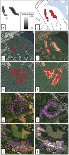
Figure 6. Example of change from to undeveloped to developed land cover isolated through change detection (a). Polygons of new developed land cover (b) are used to extract biophysical and socioeconomic variables specific to the time and place of that patch, e.g. town, area, mean vegetation fraction loss, mean slope, and residential tax rate. The polygon data is also utilized for validation of change detection in Google Earth^TM (bubble outlined in red, 2003: c and e to 2006: d and f; bust outlined in violet, 2006: g and i to 2013: h and j). For full color versions of the figures in this paper, please see the online version.

Significant loss in undeveloped land-use was mapped as individual loss patches and by each town as percentage of the town’s total area. Spatial autocorrelation and distribution of loss patch area and loss area per town was measured using Global and Local Moran’s I (Seto and Kaufman 2003). Loss patch-level Moran’s I tests were performed using inverse distance weighting using Euclidean distance and the town-level Moran’s I tests were performed using row standardized contiguity-based weighting.

Map validation

Change maps for each time period were validated with a stratified random sample of 600 points for each time period (200 per land-use stratum) with high spatial resolution imagery using Google Earth^TM (Dorais and Cardille 2011). For each land-use stratum the sample points were stratified by randomly placing 100 within loss patches and 100 outside of loss patches. Accuracy assessment is described in two levels: (I) accuracy of change or no-change maps; and (II) accuracy of change or no-change weighted by the true proportion of each land-use strata (Seto et al. 2002). The primary land-use of new development (residential or commercial) was determined with visual assessment of a random sample of 30 loss patches for each time period in Google Earth^TM.

Results

Map accuracy

Level I change/no-change accuracy assessment shows that the change maps had an overall accuracy of 88% when averaged over the study period (Table 2). The bubble time period had the highest overall level I accuracy (91%). The bust period had lower omission error than the bubble period (bubble, 5%; bust, 3%). However, the bust period commission error was 17% higher than the bubble period (bubble, 14%; bust, 31%). The main source of omission error for both time periods was decreases in vegetation cover of less than 15%, such as tree canopy loss due to storm damage or pruning. The green vegetation fraction images are likely not sensitive enough to detect these subtle changes against a background of asphalt or bare soil. Commission error for both time periods was caused primarily by detection of spurious change due to natural variability on wetlands and agriculture.

Table 2. Level I error matrix of bust and bubble period land-use change maps using Google Earth^TM data and 600 samples.

	Reference	Change	No change	Row total	Commission error
Bubble period
Classification	Change	259	41	300	0.14
	No change	13	287	300	0.04
	Column total	272	328	600
	Omission error	0.05	0.12		Overall accuracy 0.91
Bust period
Classification	Change	208	92	300	0.31
	No change	7	293	300	0.02
	Column total	215	385	600
	Omission error	0.03	0.24		Overall accuracy 0.84

The level II accuracy assessment, which evaluates change/no-change maps within the forest, urban forest, and low vegetation land-use strata, shows 28% average omission error for both time periods (Table 3). The bubble period forest change stratum had the lowest omission error (i.e., 7%), while bust period low-vegetation no-change had the highest omission error (i.e., 64%). The 64% omission error of the bust-period low-vegetation no-change stratum explains why its level I overall accuracy is low. The low-vegetation land-use stratum includes pasture and row crop agriculture, such that its map accuracy is limited by natural variability in crop fallow and rotation (Schwert et al. 2013). The bust-period level II accuracy could also have been reduced by 10% because of the 2009 land-use map used to create the land-use strata. The 2006 bust period was stratified by a 2009 land-use map resulting in change thresholds being incorrectly applied to areas that underwent change between 2006 and 2009 (Caiazzo et al. 2011).

Table 3. Level II area weighted error matrix of land-use change maps using Google Earth^TM data and 600 samples per land-use stratum: forest (orchard, hardwood, conifer, and mixed forest classes), urban forest (low- and high-density residential and commercial classes), and low vegetation (pasture/row crop, golf course, and grassland classes).

	Reference	F change	F no change	UF change	UF no change	LV change	LV no change	Samples	Map proportion
Bubble period (2000–2006)
Classification	F change	0.5386	0.0063	0.0564	0.0063	0.0125	0.0063	100	0.63
	F no change	0.0168	0.4595	0.0056	0.0729		0.0056	100	0.56
	UF change	0.0151		0.1942	0.0227	0.0101	0.0101	100	0.25
	UF no change	0.0083	0.0331	0.0055	0.2176		0.0110	100	0.28
	LV change	0.0012		0.0012		0.0887	0.0304	100	0.12
	LV no change	0.0033	0.0180		0.0443	0.0033	0.0952	100	0.16
	True proportion	0.58	0.52	0.26	0.36	0.11	0.16
	Omission error	0.07	0.12	0.25	0.40	0.19	0.40	0.20
Bust period (2006–2013)
Classification	F change	0.29027	0.01935	0.05418	0.00387	0.00774	0.01161	100	0.0011
	F no change		0.44048		0.10461	0.00551		100	0.5500
	UF change	0.03807	0.10152	0.19036	0.05499	0.03807		100	0.0012
	UF no change	0.00290	0.04345	0.00869	0.22016		0.01448	100	0.2888
	LV change	0.00570	0.00190	0.00190	0.00190	0.09498	0.08358	100	0.0006
	LV no change	0.00160	0.02396	0.00160	0.07028		0.06229	100	0.1593
	True proportion	0.34	0.63	0.26	0.46	0.15	0.17
	Omission error	0.14	0.30	0.26	0.52	0.35	0.64	0.35

Note: *F, forest; UF, urban forest; LV, low vegetation.

Land-use change

There was a significant difference in total undeveloped land-use loss between the periods of housing bubble (37.58 km²) and bust (30.29 km²) (p < 0.01). The total number of loss patches decreased by 251 (3%) and there was a 46% decrease in maximum patch area from bubble to bust, indicating that undeveloped land-use loss became more fragmented (Figure 7). The median loss patch area decreased significantly from 2700 m² during the bubble to 1800 m² in the bust period (p < 0.001), while the mean loss patch area decreased from 4848 m² to 4079 m², indicating that the top 50% of loss patches became smaller after the bubble (Table 4). Significant loss in undeveloped land-use is displayed as a percentage of town area in Figure 8. Global Moran’s I tests at the loss patch level indicate no significant difference in distribution of loss patch between bubble and bust (bubble, 0.001; bust, 0.012). Global Moran’s I tests at the town level show significant clustering during the bubble (0.274) and bust periods (0.162) (p < 0.001) of undeveloped land-use loss per town.

Table 4. Attributes and descriptive statistics of distribution of bubble and bust change maps at town and loss patch levels.

Mapping level	Minimum; maximum	Mean; median	Total	Global Moran’s I; Z-score
Bubble loss patch area (2000–2006)	1800 m^2; 428,400 m^2	4848 m^2; 2700 m^2	N = 7404	0.001; 1.90
Bust loss patch area (2006–2013)	1800 m^2; 230,400 m^2	4079 m^2; 1800 m^2	N = 7153	0.012; 1.88
Bubble (2000–2006) loss as percentage of town area	0.00%; 1.65%	0.33%; 0.28%	37.58 km^2	0.274*; 6.88
Bust (2006–2013) loss as percentage of town area	0.01%; 1.10%	0.27%; 0.23%	30.29 km^2	0.162*; 4.12

Note: *Significant at 0.01 level.

Figure 7. Map of towns with major loss of undeveloped land cover as percentage of town area (>0.85% of town area) during the bubble (a and b) and after the bubble burst (c and d). Major loss per town during the bubble was primarily attributed to large developments, while major loss per town in the bust period was primarily attributed to relatively smaller and more numerous developments.

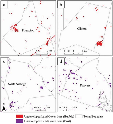
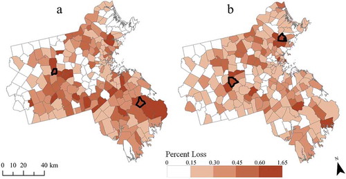
Figure 8. Map displaying loss of undeveloped land cover per town as a percentage of the town’s total area during the bubble (a) and after the bubble burst (b). Plympton, Clinton, Northborough, and Danvers (displayed in Figure 7) are outlined in black.

Small loss patches (≤ 3600 m²) observed in Google Earth^TM for both time periods included single home construction, pool installation, tree removal, and lawn/meadow mowing. Medium-to-large loss patches (> 3600 m²) included single/multifamily housing developments, office parks, shopping malls, installation of artificial turf recreation fields, and agricultural harvests. One source of conversion of undeveloped land-use found only in the bust period was the installation of solar energy farms.

Discussion

The findings of this study indicate that there was a significant difference in total area of undeveloped land-use loss between periods of housing bubble and bust. Furthermore, the spatial configuration of undeveloped land-use loss changed with the downturn in the housing market after 2006. After the bubble burst, the total number of loss patches decreased by 3%; total area of all loss patches greater than 15,000 m² decreased by 44%, and from 2005 to 2009, the number of new homes decreased by approximately 65% (US Census Bureau 2014). These changes indicate undeveloped land-use loss after the bubble occurred in smaller patches and was driven more by nonresidential development, such as shopping malls, than residential development.

The overall accuracy values (i.e., >84%) of the land change maps produced in this study allow for reasonably confident statements to be made on the area and land-use of locations of undeveloped land conversion. A study using Landsat data, the multitemporal Kauth–Thomas transformation (MKT) found 17 km² of forest cover loss from 2000 to 2005 across the entire state of Massachusetts (overall accuracy >90%; Jeon, Olofsson, and Woodcock 2014). However, the methods used in this paper detected 22 km² of undeveloped land-use loss within the forest stratum (hardwood, conifer, mixed, and orchard) from 2000 to 2006 (bust period accuracy of 84%) over an area that is 43% of the state. The discrepancy between the areas of forest loss detected in the two studies can be attributed to differences in the MKT and SMA image enhancement methods. MKT uses predefined enhancement coefficients, while SMA is scene-dependent and based on user-defined parameters (Rogan and Chen 2004). By transforming the Landsat images using SMA with biophysically significant endmembers, and deriving the change detection thresholds empirically, this study extracted the maximum available information from each scene.

The accuracy of change detection improved from an average of 59% to 84% using the change detection threshold of >10% high-albedo non-vegetation in the later year of each land change period. Naturally expanding wetlands or flooded forests were often mapped as undeveloped land-use loss, because these locations experience significant decreases in green vegetation fraction. However, little to no change in the high-albedo fraction occurs because of high absorption of visible and infrared energy by water, making the addition of the high-albedo change threshold particularly helpful for omitting natural variability of wetlands and forests from the change maps.

During the housing bubble, large commercial and multi-home residential developments were more prevalent than smaller subdivisions and single-lot development, as indicated by the higher mean and maximum loss patch areas during this period relative to the bust period. However, after the bubble burst, undeveloped land-use loss was attributed more to nonresidential construction such as shopping malls. Of the top 10 towns with the most undeveloped land loss during the bust period, seven had large shopping malls built within them. The planning, funding, and building of a large commercial development are considerably more capital-intensive in comparison to a residential neighborhood (Mulligan 2010), such that commercial development was more prevalent during the bust period. Residential development has higher profit margins than commercial development and therefore is more desirable to developers; however, after the housing bubble burst, demand for new homes diminished and construction investment and labor were allocated to commercial rather than residential development (Mulligan 2010).

Throughout both time periods, a single new home could result in as little as 1800 m² (two Landsat pixels) of undeveloped land-use loss but usually ≥ 3600 m², especially when part of a larger development. In 2006, the building footprint of the average new home in the study area is 125 m² (DeNormandie and Corcoran 2009), such that new homes can cause land change three times the size of their footprint. These findings suggest that individual homes have less wildland–urban interface than those in larger developments; however, this could be a remnant of the 30 m Landsat pixel resolution, as a single home in the study region can be built largely without disturbing the entire canopy cover of the construction site (Mockrin et al. 2013). In either configuration, the ecological footprint of the actual home spreads well beyond its physical footprint through the surrounding yard, gardens, driveway, and the everyday actions of the people and pets living there (Radeloff et al. 2005).

Conclusion

This paper set out to determine if the area of undeveloped land-use loss differs between periods of housing bubble and bust. It is difficult to directly monitor undeveloped land-use in Massachusetts, because 74% of forested land and 64% of agricultural land in the state is privately owned and managed by individuals (Kittredge et al. 2008; DeNormandie and Corcoran 2009). Furthermore, the state holds a home rule charter insuring the autonomy of each town in planning and funding land-use, resulting in distinct land-use patterns of development between towns. As a result, land-use change in Massachusetts is often the result of complex interaction between individuals and municipal government, rather than at the county or state level (Rogan et al. 2013; McCauley et al. 2015). The findings of this research show that the total area and geographic distribution of undeveloped land-use loss decreases from periods of economic bubble to bust. Availability of housing is a key factor in maintaining a thriving economy and labor force (Bluestone et al. 2012; Fitzgerald 2013). As governments seek to maintain a competitive economy, it is critical to uphold and perhaps enhance regulations surrounding preservation and development of undeveloped land. Land-use and protection policies should not be curtailed due to fluctuations in the real estate market or to encourage economic growth.

Disclosure statement

No potential conflict of interest was reported by the authors.

Acknowledgments

The author would like to acknowledge the Clark University Graduate School of Geography and previous work by the HERO program and the Massachusetts Forest Monitoring Program, without which this material would not be possible. Thanks to the three anonymous reviewers whose helpful comments have improved the quality of this manuscript. All findings expressed in this material are those of the authors and do not necessarily reflect the view of the funders

Additional information

Funding

This work was funded by the National Science Foundation (NSF) [grant number SES-0849985] (REU Site); the Clark University O’Connor ’78 Endowment.

References

- Abdullahi, S., B. Pradhan, S. Mansor, and A. Shariff. 2015. “Gis-Based Modeling for the Spatial Measurement and Evaluation of Mixed Land Use Development for a Compact City.” GIScience & Remote Sensing 52 (1): 18–39. doi:10.1080/15481603.2014.993854.
- Aber, J., C. Cogbill, E. Colburn, A. D’Amato, B. Donahue, C. Driscoll, A. Ellison, et al. 2010. Wildlands and Woodlands: A Vision for the New England Landscape. Petersham, MA: Harvard University Press. http://www.wildlandsandwoodlands.org/sites/default/files/Wildlands%20and%20Woodlands%20New%20England.pdf
- Adams, J. B., D. Sabol, V. Kapos, R. Filho, D. Roberts, M. Smith, and A. Gillespie. 1995. “Classification of Multispectral Images Based on Fractions of Endmembers: Application to Land-Cover Change in the Brazilian Amazon.” Remote Sensing of Environment 52 (2): 137–154. doi:10.1016/0034-4257(94)00098-8.
- Baker, D. 2005. “The Housing Bubble Fact Sheet.” Center for Economic and Policy Research ((Issue Brief)): 1–5. http://www.cepr.net/documents/publications/housing_fact_2005_07.pdf
- Baldridge, A. M., S. J. Hook, C. I. Grove, and G. Rivera. 2009. “The ASTER Spectral Library Version 2.0.” Remote Sensing of Environment 113 (4): 711–715. doi:10.1016/j.rse.2008.11.007.
- Bluestone, B., C. Billingham, E. White, M. Siflinger, T. Davis, and T. Reardon. 2012. “A New New Paradigm for Housing in Greater Boston.” The Greater Boston Housing Report Card 10: 1–94. http://www.tbf.org/~/media/TBFOrg/Files/Reports/2012%20Housing%20RC_Nov01.pdf
- Caiazzo, A., J. Rogan, Y. Ogneva-Himmelberger, C. Woodcock, and S. Ratick. 2011. “A New Method for Pre-Dating and Post-Dating Land Cover Maps with Landsat and Aster Imagery Using a Kauth-Thomas Change Index.” Master’s Thesis, Clark University.
- Chavez, P. 1996. “Image-Based Atmospheric Corrections: Revisited and Improved.” Photogrammetric Engineering & Remote Sensing 62 (9): 1025–1036.
- Cohen, W., and S. Goward. 2004. “Landsat’s Role in Ecological Applications of Remote Sensing.” Bioscience 54 (6): 535–545. doi:10.1641/0006-3568(2004)054[0535:LRIEAO]2.
- DeNormandie, J., and C. Corcoran. 2009. “Losing Ground: Beyond the Footprint.” Mass Audubon. http://www.massaudubon.org/content/download/8601/149722/file/LosingGround_print.pdf
- Dodds, K., and D. Orwig. 2011. “An Invasive Urban Forest Pest Invades Natural Environments— Asian Longhorned Beetle in Northeastern US Hardwood Forests.” Canadian Journal of Forest Research 41 (9): 1729–1742. doi:10.1139/x11-097.
- Dokko, J., B. Doyle, M. Kiley, J. Kim, S. Sherlund, J. Sim, and S. Van Den Heuvel. 2011. “Monetary Policy and the Global Housing Bubble.” Economic Policy 26 (66): 237–287. doi:10.1111/j.1468-0327.2011.00262.x.
- Dorais, A., and J. Cardille. 2011. “Strategies for Incorporating High-Resolution Google Earth Databases to Guide and Validate Classifications: Understanding Deforestation in Borneo.” Remote Sensing 3 (12): 1157–1176. doi:10.3390/rs3061157.
- Fitzgerald, J. 2013. “Are We Creating the Next Housing Bubble in Massachusetts?” The Boston Globe, June 30. http://www.bostonglobe.com/business/2013/06/29/are-heading-another-housing-bubble/A8njF4efabncV58g25SM6K/story.html
- Foster, D., D. Kittredge, B. Donahue, G. Motzkin, D. Orwig, A. Ellison, B. Hall, B. Colburn, and A. D’Amato. 2005. Wildlands and Woodlands: A Vision for the Forests of Massachusetts. Petersham, MA: Harvard University Press. http://www.wildlandsandwoodlands.org/sites/default/files/Wildlands%20%26%20Woodlands%20Massachusetts.pdf
- Gagné, S., and L. Fahrig. 2011. “Do Birds and Beetles Show Similar Responses to Urbanization?” Ecological Applications 21 (6): 2297–2312. doi:10.1890/09-1905.1.
- Gavier-Pizarro, G., V. Radeloff, S. Stewart, C. Huebner, and N. Keuler. 2010. “Housing is Positively Associated with Invasive Exotic Plant Species Richness in New England, USA.” Ecological Society of America 20 (7): 1913–1925. doi:10.1890/09-2168.1.
- Giner, N., and J. Rogan. 2012. “A Comparison of Landsat Etm+ And High-Resolution Aerial Orthophotos to Map Urban/Suburban Forest Cover in Massachusetts, USA.” Remote Sensing Letters 3 (8): 667–676. doi:10.1080/01431161.2012.656767.
- Glaeser, E., J. Gottleb, and J. Gyourko. 2010. “Can Cheap Credit Explain the Housing Boom?” National Bureau of Economic Research, July. http://www.nber.org/papers/w16230.pdf
- Google Inc. 2014. Google EarthTM Version: 7.1.2. 2041. https://www.google.com/earth/
- Hostetler, A., J. Rogan, D. Martin, V. DeLauer, and J. O’Neil-Dunne. 2013. “Characterizing Tree Canopy Loss Using Multi-Source GIS Data in Central Massachusetts, USA.” Remote Sensing Letters 4 (12): 1137–1146. doi:10.1080/2150704X.2013.852704.
- Jeon, S. B., P. Olofsson, and C. Woodcock. 2014. “Land Use Change in New England: A Reversal of the Forest Transition.” Journal of Land Use Science 9 (1): 105–130. doi:10.1080/1747423X.2012.754962.
- Kittredge, D., A. D’Amato, P. Catanzaro, J. Fish, and B. Butler. 2008. “Estimating Ownerships and Parcels of Nonindustrial Private Forestland in Massachusetts.” Northern Journal of Applied Forestry 25 (2): 93–98.
- Levitin, A., and S. Wachter. 2012. “Explaining the Housing Bubble.” Georgetown Law Journal 100 (4): 1177–1258. http://papers.ssrn.com/sol3/papers.cfm?abstract_id=1669401
- MaFoMP. 2011. “Massachusetts Forest Monitoring Program (MaFoMP), Human-Environment Regional Observatory of Central Massachusetts (HERO-CM).” http://www.clarku.edu/department/hero/researcharea/forestchange.cfm
- Massachusetts Department of Agricultural Resources. 2014. “Agricultural resources facts and statistics.” http://www.mass.gov/eea/agencies/agr/statistics/
- McCauley, S., J. Rogan, J. Murphy, B. Turner, and S. Ratick. 2015. “Modeling the Sociospatial Constraints on Land-use Change: The Case of Periurban Sprawl in the Greater Boston Region.” Environment and Planning B: Planning and Design 42 (2): 221–241. doi:10.1068/b38018.
- Mockrin, M., S. Stewart, V. Radeloff, R. Hammer, and K. Johnson. 2013. “Spatial and Temporal Residential Density Patterns From 1940 to 2000 in and Around the Northern Forest of the Northeastern United States.” Population and Environment 34 (3): 400–419. doi:10.1007/s11111-012-0165-5.
- Mulligan, C. 2010. “Was There a Commercial Real Estate Bubble?” The New York Times, January 13. http://economix.blogs.nytimes.com/2010/01/13/was-there-a-commercial-real-estate-bubble/?_php=true&_type=blogs&_r=0
- Nowak, D., J. Wang, and T. Endreny. 2007. “Environmental and Economic Benefits of Preserving Forests Within Urban Areas: Air and Water Quality.” Chapter 4 in The Economic Benefits of Regional Land Conservation, 28–47. http://www.nrs.fs.fed.us/pubs/jrnl/2007/nrs_2007_nowak_002.pdf
- Pimentel, D., R. Zuniga, and D. Morrison. 2005. “Update on the Environmental and Economic Costs Associated with Alien-Invasive Species in the United States.” Ecological Economics 52 (3): 273–288. doi:10.1016/j.ecolecon.2004.10.002.
- Radeloff, V., R. Hammer, S. Stewart, J. Fried, S. Holcomb, and J. McKeefry. 2005. “The Wildland-Urban Interface in the United States.” The Ecological Society of America 15 (3): 799–805. doi:10.1890/04-1413.
- Radeloff, V., E. Nelson, A. Plantinga, D. Lewis, D. Helmers, J. Lawler, and J. Withey, et al. 2012. “Economic-Based Projections of Future Land Use in the Conterminous United States Under Alternative Policy Scenarios.” The Ecological Society of America 22 (3): 1036–1049. doi:10.1890/11-0306.1.
- Radeloff, V., S. Stewart, T. Hawbaker, U. Gimmi, A. Pidgeon, C. Flather, R. Hammer, and D. Helmers. 2010. “Housing Growth in and near United States Protected Areas Limits Their Conservation Value.” Proceedings of the National Academy of Sciences of the United States of America 107 (2): 940–945. doi:10.1073/pnas.0911131107.
- Rogan, J., and D. Chen. 2004. “Remote Sensing Technology for Mapping and Monitoring Land-Cover and Land-Use Change.” Progress in Planning 61: 301–325. doi:10.1016/S0305-9006(03)00066-7.
- Rogan, J., M. Ziemer, D. Martin, S. Ratick, N. Cuba, and V. DeLauer. 2013. “The Impact of Tree Cover Loss on Land Surface Temperature: A Case Study of Central Massachusetts Using Landsat Thematic Mapper Thermal Data.” Applied Geography 45: 49–57. doi:10.1016/j.apgeog.2013.07.004.
- Schneider, A. 2012. “Monitoring Land Cover Change in Urban and Peri-Urban Areas Using Dense Time Stacks of Landsat Satellite Data and a Data Mining Approach.” Remote Sensing of Environment 124: 689–704. doi:10.1016/j.rse.2012.06.006.
- Schwert, B., J. Rogan, N. Giner, Y. Ogneva-Himmelberger, S. Blanchard, and C. Woodcock. 2013. “A Comparison of Support Vector Machines and Manual Change Detection for Land-Cover Map Updating in Massachusetts, USA.” Remote Sensing Letters 4 (9): 882–890. doi:10.1080/2150704X.2013.809497.
- Seto, K., and R. Kaufman. 2003. “Modeling the Drivers of Urban Land Change in the Pearl River Delta, China.” Land Economics 79 (1): 106–121. doi:10.2307/3147108.
- Seto, K., C. Woodcock, C. Song, X. Huang, J. Lu, and R. Kaufman. 2002. “Monitoring Land-Use Change in the Pearl River Delta Using Landsat TM.” International Journal of Remote Sensing 23 (10): 1985–2004. doi:10.1080/01431160110075532.
- Settle, J. J., and N. A. Drake. 1993. “Linear Mixing and the Estimation of Ground Cover Proportions.” International Journal of Remote Sensing 14 (6): 1159–1177. doi:10.1080/01431169308904402.
- Slonecker, T., L. Milheim, and P. Claggett. 2010. “Landscape Indicators and Land Cover Change in the Mid-Atlantic Region of the United States, 1973-2001.” GIScience & Remote Sensing 47 (2): 163–186. doi:10.2747/1548-1603.47.2.163.
- Small, C. 2001. “Estimation of Urban Vegetation Abundance by Spectral Mixture Analysis.” International Journal of Remote Sensing 22 (7): 1305–1334. doi:10.1080/01431160151144369.
- US Census Bureau. 2010. “State & County Quickfacts: Massachusetts.” http://www.census.gov/2010census/data/
- US Census Bureau. 2014. “Building Permits Data.” http://censtats.census.gov/
- US Department of Commerce. 2014. “Contributions to percent change in real gross domestic product data.” http://www.bea.gov/iTable/iTable.cfm?ReqID=9&step=1#reqid=9&step=3&isuri=1&903=2.
- Václavík, T., and J. Rogan. 2009. “Identifying Trends in Land Use/Land Cover Changes in the Context of Post-Socialist Transformation in Central Europe: A Case Study of the Greater Olomouc Region, Czech Republic.” GIScience & Remote Sensing 46 (1): 54–76. doi:10.2747/1548-1603.46.1.54.
- Weng, Q. 2012. “Remote Sensing of Impervious Surfaces in the Urban Areas: Requirements, Methods, and Trends.” Remote Sensing of Environment 117: 34–49. doi:10.1016/j.rse.2011.02.030.