Effects of analytical window and resolution on topographic relief derived using digital elevation models

Abstract

Relief has been used as an index to quantify the vertical dimension of topography in landscape evolution studies. However, potential impacts of analytical window and resolution of digital elevation models (DEMs) were seldom addressed. Here, three relief parameters (fixed-area local relief, watershed relief, and watershed mean local relief) were examined for three topographic regions (relatively flat loess-till plains in northern Missouri, hilly karst topography in southern Missouri, and a mountainous topography in western Washington) using DEMs of 30-m (USGS NED), 90-m (SRTM), and 1-km (GTOPO30), which are commonly applied in landscape evolution studies. Results indicate that both fixed-area and watershed mean local reliefs are strongly affected by the size of the analytical window, whereas watershed relief is relatively stable. The correlation between watershed relief and watershed mean local relief is affected by the edge effect in determining watershed mean local relief, especially for small watersheds. The comparisons between relief parameters derived from these three resolution DEMs indicate <5% difference between 30- and 90-m DEMs, but >15% difference between 30-m and 1-km DEMs. The relatively large disparity may affect the suitability of using the 1-km GTOPO30 DEM in relief determination.

Keywords:

• topographic relief
• DEM
• GIS
• edge effect
• watershed

1. Introduction

Topographic relief has been widely used in landscape classification and long-term landscape evolution studies (e.g., Montgomery and Brandon 2002; Matmon et al. 2003; Vance et al. 2003; Aalto, Dunne, and Guyot 2006; Finnegan et al. 2008; Henck et al. 2011; Li et al. 2014). It is initially defined as a simple description of the vertical dimension of topography (e.g., Smith 1935). With the development of various methods to quantify basin sediment yield and denudation rates, such as sediment measurements from dam/reservoirs (Dendy and Champion 1978; Steffen 1996) and long-term denudation rates constrained by cosmogenic nuclides (Bierman and Nichols 2004; von Blanckenburg 2005; Li et al. 2014) and low-temperature thermochronometry (Brandon, Roden-Tice, and Garver 1998; Ehlers and Farley 2003; Spotila 2005), it has become an important topographic index in quantifying landscape denudation rates (e.g., Schumm 1956; Ahnert 1970; Schaller et al. 2001; Montgomery and Brandon 2002; Vance et al. 2003; Aalto, Dunne, and Guyot 2006; Finnegan et al. 2008). In general, two types of relief parameters have been used to examine the landscape denudation-topography relationship. The first is defined for a location as the maximum elevation difference within an arbitrary analytical window, such as a 10-km-diameter circle (Montgomery and Brandon 2002; Aalto, Dunne, and Guyot 2006; Finnegan et al. 2008) or a 20×20 km square (Ahnert 1970), around this location (named as fixed-area local relief in this paper). The second type is defined for an area. In this perspective, watershed (basin) relief, the maximum elevation difference within a watershed, is commonly used (Hadley and Schumm 1961; Schumm 1956, 1963). Due to the size difference, watershed relief is usually normalized by the area or the length of the watershed. For example, relief ratio, a dimensionless parameter defined as watershed relief divided by basin length, has been used to compare watershed reliefs of varying sizes (Schumm 1956, 1963). Ahnert (1970) argued that relief ratio is probably not a good measure for large watersheds because two watersheds may have nearly the same relief ratio, but differ greatly within the basin where mountainous terrain occupies only a small portion of one watershed, but a very large part of the other watershed. Instead, he introduced a watershed mean local relief, defined as the averaged fixed-area local relief of all cells within the watershed based on an analytical window, to avoid this potential issue (Ahnert 1970).

The use of relief parameters has significantly improved our understanding of the relationship between landscape denudation and topography. For example, Ahnert (1970) reported a linear relationship between erosion rate and watershed mean local relief for mid-latitude watersheds using a 20×20 km square as the analytical window. Montgomery and Brandon (2002) proposed a nonlinear relationship between erosion rate and fixed-area local relief derived using a 10-km-diameter circle. Vance et al. (2003) introduced a log-linear relationship between long-term denudation rates measured by cosmogenic nuclides and modified watershed mean local relief determined by the difference between the mean and the minimum elevations using an analytical window of a 9×9 km square. Li et al. (2014) reported a decoupled denudation-topography relationship for relatively large drainage basins in an arid region of the northern Tibetan Plateau due to retarded sediment transportation and prolonged sediment storage.

Most relief parameters (except watershed relief) require a subjectively defined analytical window, but the size effect of the analytical window was seldom addressed. Evans (1972) provided an initial assessment of the size effect of the analytical window by comparing fixed-area local reliefs derived from various windows and pointed out that a small window would possibly not contain a whole slope of the topography, so that the derived relief is simply a measure of slope gradient. He recommended using a “fairly large” window to cover both valleys and interfluves in the relief determination. Up to now, different sizes and shapes of analytical windows have been used in landscape denudation studies, such as a 20×20 km square (Ahnert 1970), a 10-km-diameter circle (Montgomery and Brandon 2002; Aalto, Dunne, and Guyot 2006; Finnegan et al. 2008), and a 9×9 km square (Schaller et al. 2001; Vance et al. 2003). However, the use of these arbitrary windows has been mainly based on subjective preferences without a detailed investigation of the impacts of different choices on relief determination. In addition, most studies have focused on a certain type of topography (Ahnert 1970; Evans 1972; Schaller et al. 2001; Vance et al. 2003), while potential variations across different types of topography (for example, the comparison between relatively flat area and mountainous topography) were seldom discussed. Furthermore, studies have indicated that DEM-derived parameters may behave differently across different resolutions. For example, slope has proved very sensitive to DEM resolutions, whereas the watershed/basin area and hypsometric integral are relatively stable for different resolutions (Zhang and Montgomery 1994; Hammer et al. 1995; Hurtrez, Sol, and Lucazeau 1999; Walker and Willgoose 1999; Zhang et al. 1999; Yin and Wang 1999; Montgomery and Brandon 2002). Some studies also suggested that relief is a relatively stable parameter across different resolutions (Polidori, Chorowicz, and Guillande 1991; Montgomery and Brandon 2002), but it still lacks a systematic examination of the resolution effect on relief parameters, although it is of critical importance in better understanding of the relationship between landscape denudation and topography.

The purpose of this study is to assess the impacts of different analytical windows and DEM resolutions on the determination of fixed-area local relief, watershed relief, and watershed mean local relief for three topographic types (relatively flat loess-till plains in the northern Missouri, hilly karst topography in the southern Missouri, and a mountainous topography in the western Washington). This assessment is conducted for three DEM resolutions of 30-m, 90-m, and 1-km that have been commonly used in long-term landscape denudation studies.

2. Study areas

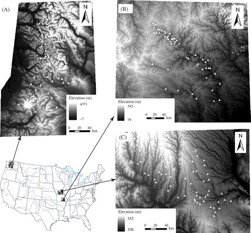
Three topographic areas were selected to examine the relationships between different relief parameters and the impacts of analytical windows and DEM resolutions (Figure 1). The first is from the Cascade Range in the western Washington with an overall relief of >2000 m (Figure 1A). This area represents a typical mountainous topography with strong tectonic uplift and volcanic activities. The topographic, geologic, and thermochronometric evidence suggests a polygenetic topography development history interplayed between tectonic uplift and post-uplift erosion in this mountain range (Mitchell and Montgomery 2006). The second area is dissected karst topography from the Ozark Plateau in the southern Missouri with an overall relief of 400–500 m (Figure 1B). The Ozark Plateau is the most extensive mountainous topography between the Appalachians and the Rocky Mountains in the US, covering the southern Missouri and the central-northern Arkansas. The third area is from loess-till plains in the northern Missouri with an overall relief of <250 m (Figure 1C). The loess-till plains, represented as gentle rolling hills, were formed by glacial deposits of the past ice sheet and later loess accumulation during the last glacial cycle.

Figure 1. Study areas and selected points in each area: (A) the Cascade Range in the western Washington; (B) the Ozark Plateau in the southern Missouri; and (C) the loess-till plains in the northern Missouri. Triangles in each panel indicated the selected points used to determine fixed-area local relief, watershed relief, and watershed mean local relief.

3. Data description and methods

Different types of DEMs have been generated based on various techniques, such as ground survey, photogrammetry, interferometric synthetic aperture radar, and LiDAR (Light Detection and Ranging) (e.g., Shaker, Yan, and Easa 2010; Stefanik et al. 2011; Xie, Pearlstine, and Gawlik 2012). These DEMs have different resolutions, ranging from sub-meters to kilometers, and the DEM accuracy is affected by data sources, quality, as well as the interpolation methods and parameters in producing the topography (e.g., Shaker, Yan, and Easa 2010; Chirico, Malpeli, and Trimble 2012; Gómez et al. 2012; Gosciewski 2013). Therefore, it is difficult to assess the impacts of analytical window and resolution on relief parameters for all available DEMs. In this study, I focus on three types of DEMs that are commonly applied in landscape evolution studies: (1) 1 arc-second (30-m) resolution DEM downloaded from the USGS National Elevation Dataset (NED) (http://nationalmap.gov/viewer.html); (2) 3 arc-second (90-m) resolution Shuttle Radar Topography Mission (SRTM) DEM (http://srtm.csi.cgiar.org); and (3) 30 arc-second (about 1-km) GTOPO30 DEM (https://lta.cr.usgs.gov/GTOPO30). The downloaded DEMs were first re-projected to the Universal Transverse Mercator (UTM) projection and extracted for each study area using a predefined boundary. Since landscape denudation rates have been mainly measured from stream sediments, the focus of this study is to derive and compare relief parameters along the valley (stream). I used ArcGIS hydrology tools (e.g., flow direction and flow accumulation) to help delineate the stream network and identify the valleys, and then selected fifty points from different valleys in each area to determine their fixed-area local relief, watershed relief, and watershed mean local relief values. These values were used to examine different relief parameters and assess the impacts of analytical windows and DEM resolutions. The reason for processing fifty points in each area is to allow for the statistical comparison between relief parameters derived using different analytical windows and DEM resolutions, and to limit the computational power required for the analysis.

3.1. Fixed-area local relief

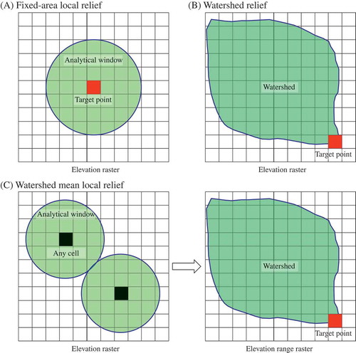
In this study, fixed-area local relief is defined as the maximum elevation difference around a location (point) using a circular analytical window (Figure 2A). It can be derived using the elevation values extracted within a buffer distance (analytical window) around a location. To represent the relief characteristics for a topographic area, the mean and standard deviation of the fixed-area local relief values from multiple locations (50 points in this paper) were used to mitigate the local influence on this relief parameter at any specific point. The mean value of the fixed-area local relief values is defined as

(1)

Figure 2. Diagrams illustrating the three relief parameters used in this study: (A) fixed-area local relief defined as the maximum elevation difference around a target point using a circular analytical window; (B) watershed relief defined as the maximum elevation difference within a watershed; and (C) watershed mean local relief defined as the averaged fixed-area local relief of all cells within a watershed using a specified analytical window. Two steps are needed to derive this parameter: (1) creating an elevation range raster (fixed-area local relief for each cell) from the DEM based on the specified window; and (2) extracting all values with the watershed to calculate the watershed mean local relief. For full color versions of the figures in this paper, please see the online version.

where µ is the mean value, R_i is the fixed-area local relief determined for point i, n is the number of points (n = 50). The standard deviation (σ) of the fixed-area local relief values is defined as

(2)

The standard deviation describes the variability of relief values among different points, but it is unit-based and amplified depending on the scale of the mean (Djebou, Singh, and Frauenfeld 2014). This issue can be corrected using the coefficient of variation (CV), defined as the ratio of the standard deviation to the mean (CV = σ/µ). It is a dimensionless number and can be used to compare between datasets with different units or widely different means (Djebou, Singh, and Frauenfeld 2014). Thus, the coefficient of variation was used to assess the impacts of buffer diameters and DEM resolutions on the variability of the fixed-area local reliefs derived from different points in each topographic area.

To implement the analysis, a set of buffers was first created for each point using diameters from 1 km to 25 km with an interval of 1 km. For the GTOPO30 DEM, due to its relatively coarse resolution (about 1-km), the buffer diameter was started from 2 km. Then, fixed-area local relief values were calculated for different buffers to examine the impact of analytical windows and DEM resolutions on this relief parameter in each area.

3.2. Watershed relief

Watershed relief is defined as the maximum elevation difference within a watershed (Figure 2B). Due to the size difference, in this study, watershed relief is normalized using the square root of the watershed area (Melton 1965):

(3)

where R_ws is the normalized watershed relief, E_max and E_min are the maximum and minimum elevations within the watershed, respectively, and A is the watershed area. R_ws is a dimensionless parameter similar to the relief ratio introduced by Schumm (1956).

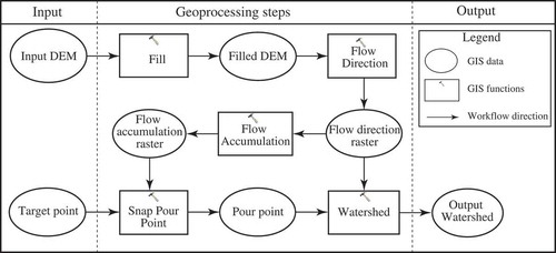
To derive R_ws, the upland watershed corresponding to each point was delineated in ArcGIS using the standard D-8 algorithm by assigning a flow direction to each DEM cell based on the steepest downhill slope (Tribe 1992). Figure 3 illustrates the whole watershed delineation processes for a target point in ArcGIS, including: (1) filling potential DEM sinks to make sure each DEM cell has a single outflow direction; (2) calculating flow direction and accumulation to record the outflow direction and the total number of cells flowing into a certain DEM cell; and (3) determining the watershed boundary for each point (as a pour point). The delineated watershed area and extracted elevations within the watershed were used to calculate the R_ws for the upland watershed of each point.

Figure 3. An ArcGIS flowchart to delineate the watershed boundary for a target point.

3.3. Watershed mean local relief

Watershed mean local relief is defined as the averaged fixed-area local relief of all cells within a watershed using a specified analytical window (Figure 2C). To account for the size difference of the watershed, it is also normalized using the square root of the watershed area in this paper, similar to the treatment for the watershed relief. However, different from watershed relief that has only one value for a watershed in a DEM, watershed mean local relief is associated with the assigned analytical window and multiple values can be derived for different windows.

Two potential approaches can be used to derive watershed mean local relief. One is to first calculate the fixed-area local relief for each cell using an analytical window and then calculate the mean fixed-area local relief for all cells within the watershed (Figure 2C). The other is to first extract the DEM within a watershed and then calculate the fixed-area local relief for each cell to determine the mean fixed-area local relief for the watershed. I used the first approach in this study because it is commonly used in landscape denudation studies to derive watershed mean local relief (e.g., Aalto, Dunne, and Guyot 2006; Henck et al. 2011; Li et al. 2014). To derive the watershed mean local relief for each point, the Focal Range function in ArcGIS was first used to determine the fixed-area local relief for each cell in the DEM (Figure 2C). This function finds the range of elevations within the specified window and assigns this value to the center cell. Then, the watershed boundary for each point was used to extract the fixed-area local relief values within the watershed to calculate and normalize the watershed mean local relief (Figure 2C). In this study, watershed mean local relief was calculated for buffer diameters of 3, 5, 8, 10, 15, and 20 km, respectively, to examine the impact of analytical window.

3.4. Relief comparison and statistical analysis

Scatter plots were used to visually examine the relationships between relief parameters derived using different analytical windows and DEM resolutions. Pearson correlation analysis was conducted to quantify the correlations between relief parameters derived using different analytical windows and resolutions, and the correlation coefficient, r, was used to evaluate the strength and direction of the correlation. The p-values (significance levels) of most correlations are <0.01 (Tables 2 and 3; Figure 4). Thus, the significance level for each correlation was not discussed in the text.

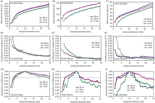
Figure 4. Relationships between fixed-area local relief and analytical window. Panels A, B, C are for the mean relief value; panels D, E, F are for the coefficient of variation (CV); and panels G, H, I are for the correlation coefficient (r) between the relief values of each window and the values of the 10-km analytical window (the p-values of most correlations are <0.01). The left three panels (A, D, G) are for the Cascade Range in the western Washington; the middle three panels (B, E, H) are for the Ozark Plateau in the southern Missouri; and the right three panels (C, F, I) are for the loess-till plains in the northern Missouri. Different curves in each panel are from different DEM resolutions.

To quantify the difference between relief values derived using different resolutions, the relief value derived from the 30-m DEM, the finest resolution of these three DEMs, was treated as the reference value. Relief values derived from 90-m and 1-km DEMs were compared to this reference value. Both absolute and relative differences (defined as the ratio of the absolute difference to the reference value) were calculated to quantify the disparity between different DEM resolutions.

4. Results and discussion

4.1. Fixed-area local relief

The relationship between fixed-area local relief and analytical window indicates similar trends for different topographic types and DEM resolutions (Figure 4A–C). Basically, the mean of fixed-area local relief values in each area continuously increases with the increased analytical window. A “turning point” occurs when the analytical window increases to a threshold, changing the relief-increasing rate to a reduced value after the window is continuously getting larger. This is similar to the observation of Wood and Snell (1960) in the determination of topographic grain and Evans’ (1972) work in assessing the analytical window effect on local relief. If the analytical window is smaller than this threshold, it may not cover both valleys and interfluves and the derived relief is simply a measure of slope gradient. In contrast, a larger window than this threshold would cover both of them to produce a representative relief parameter for a location. Our results indicate that different topographic types require different thresholds. Specifically, the thresholds are about 5–6 km, 3–4 km, and 2–3 km for the mountainous area in the Cascade Range, the karst topography in the southern Missouri, and the loess-till plains in the northern Missouri, respectively. In general, higher topographic relief areas require larger analytical windows to cover both valleys and interfluves.

The coefficient of variation (CV) of relief values decreases with the increased analytical window in each area (Figure 4D–F). This decreasing trend may indicate that another threshold exists in the analytical window. When the analytical window is larger than this threshold, the coefficient of variation almost reaches a constant value, becoming independent from the continuously increasing analytical window. For example, in the mountainous area of the Cascade Range (Figure 4D), the coefficient of variation continuously decreases with the increasing buffer diameter, but when the diameter is >16 km, it reaches a relatively constant value around 0.20. Similar thresholds for the karst topography and the loess-till plains are around 10 and 5 km, respectively (Figure 4E and F). The existence of this threshold indicates that if the analytical window is too large, local relief determined for each site may be over-generalized for discriminating the difference between different sites.

If the existence of the first mentioned threshold indicates that a fairly large analytical window is necessary to represent local relief appropriately, the existence of the second threshold suggests that the window could not be too large to avoid the over generalization of the relief parameter. These two thresholds provide a useful guidance in determining an appropriate window for fixed-area local relief analysis. Due to the common use of a 10-km-diameter circle as the analytical window in landscape denudation studies (e.g., Montgomery and Brandon 2002; Aalto, Dunne, and Guyot 2006; Finnegan et al. 2008), Pearson correlation analysis was conducted to examine if the relief value derived using this window correlates well with the values derived from other windows (Figure 4G–I), so that it can be representative for local relief characteristics around a location. Results indicate a strong correlation (r > 0.8) from 3 to 25 km for the 30- and 90-m DEMs and 4–23 km for the 1-km DEM in the mountainous topography of the Cascade Range (Figure 4G). Correlations in the karst topography and loess-till plains are relatively weak. For the karst topography, relief derived using the 10-km window correlates well (r > 0.8) for 3–13 km for the 30- and 90-m DEMs and 6–12 km for the 1-km DEM (Figure 4H). For the loess-till plains, it correlates well (r > 0.8) for 3–19 km for the 30-m DEM, 5–13 km for the 90-m DEM, and 8–13 km for the 1-km DEM (Figure 4I). These results suggest that a simple treatment to derive fixed-area local relief using a predefined analytical window (such as a 10-km-diameter circle) may be not suitable for different topographic types. A detailed examination of the relationship between relief and analytical window is recommended to determine the appropriate window before conducting the fixed-area local relief analysis.

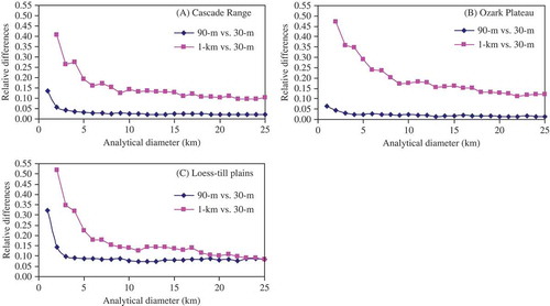
As illustrated in Figure 4A–F, the relief values for 30 and 90-m DEM resolutions were almost identical (except for the loess-till plains), but significantly different from the 1-km DEM. The relative differences between relief value derived from 90-m or 1-km DEMs to the reference value derived using 30-m DEM indicate <5% differences (corresponding to a ratio of 0.05) between 90- and 30-m DEMs, but >15% differences (corresponding to a ratio of 0.15) between 1-km and 30-m DEMs for the Cascade Range (Figure 5A) and the karst topography (Figure 5B). For the loess-till plains, the relative difference between 90- and 30-m DEMs is relatively high (mostly 8–10%, Figure 5C), but the absolute difference between 90- and 30-m DEMs for each site in this area is relatively small (<6 m in average) because of the relatively flat topography. This indicated that the 90-m DEM could be used as a substitute for the 30-m DEM in relief analysis where the 30-m DEM is unavailable or for relatively large areas that require significant computational power to process the 30-m DEM. In contrast, the relatively large disparity between local relief values derived from the 1-km DEM and the 30-m DEM may affect the suitability of using the 1-km DEM in fixed-area local relief analysis.

Figure 5. Relative differences between 90-m, 1-km, and 30-m DEMs and their variations in different analytical windows: (A) the Cascade Range in the western Washington; (B) the Ozark Plateau in the southern Missouri; and (C) the loess-till plains in the northern Missouri. Different curves in each panel are for different DEM resolutions.

4.2. Watershed relief and watershed mean local relief

Watershed relief is a relatively stable parameter without the influence of the analytical window. Table 1 listed the relative difference of the normalized watershed relief (normalized by the square root of the watershed area) of 90-m and 1-km DEMs compared to the 30-m DEM. Similar to results discussed for fixed-area local relief, relative differences between 90- and 30-m DEMs are relatively small (<5%, corresponding to a ratio of 0.05), whereas relative differences between 1-km and 30-m DEMs are fairly significant (>15%, corresponding to a ratio of 0.15).

Table 1. Relative difference of normalized watershed reliefs of 90-m and 1-km DEMs compared to the reference value derived from the 30-m DEM (calculated as the ratio of the absolute difference to the reference value).

	STRM 90-m DEM				GTOPO 1-km DEM
	Mean	Min	Max	STD	Mean	Min	Max	STD
Western Washington	0.04	0.01	0.14	0.03	0.16	0.00	0.42	0.09
Southern Missouri	0.02	0.00	0.08	0.02	0.35	0.04	0.91	0.28
Northern Missouri	0.04	0.00	0.31	0.05	0.19	0.00	1.04	0.20

Note: Min: Minimum difference; Max: Maximum difference; STD: Standard deviation.

Different from watershed relief that only has one value for each basin in a DEM, watershed mean local relief has multiple values for difference analytical windows. Therefore, watershed mean local relief may be also affected by the size of analytical window. As listed in Table 2, the r values (all positive, indicating positive correlations) between the watershed mean local reliefs derived from two buffer diameters usually decrease with the increased difference in buffer diameters. Most r values are over 0.80, indicating fairly strong correlations between watershed mean local reliefs derived from different analytical windows.

Table 2. Correlation coefficient (r) between watershed mean local relief values derived using different diameters. The left, middle, and right values (separated by “/”) are for different DEM resolutions of 30-m, 90-m and 1-km, respectively (the p-values for all correlations are <0.01).

	3-km	5-km	8-km	10-km	15-km	20-km
(a) Western Washington
3-km	1	0.99/0.99/0.99	0.95/0.95/0.94	0.92/0.91/0.90	0.81/0.80/0.82	0.71/0.69/0.70
5-km		1	0.98/0.98/0.97	0.95/0.95/0.93	0.87/0.85/0.85	0.76/0.75/0.73
8-km			1	0.99/0.99/0.99	0.93/0.93/0.94	0.83/0.83/0.83
10-km				1	0.96/0.96/0.98	0.88/0.87/0.87
15-km					1	0.97/0.97/0.94
20-km						1
(b) Southern Missouri
3-km	1	0.99/0.99/0.99	0.94/0.94/0.95	0.88/0.88/0.92	0.75/0.74/0.84	0.71/0.71/0.78
5-km		1	0.97/0.97/0.97	0.93/0.93/0.94	0.82/0.80/0.87	0.77/0.75/0.81
8-km			1	0.98/0.98/0.99	0.92/0.90/0.93	0.87/0.86/0.88
10-km				1	0.96/0.95/0.97	0.92/0.92/0.93
15-km					1	0.98/0.98/0.98
20-km						1
(c) Northern Missouri
3-km	1	0.99/0.99/0.97	0.99/0.98/0.91	0.98/0.97/0.87	0.95/0.94/0.81	0.91/0.89/0.73
5-km		1	0.99/0.99/0.95	0.99/0.98/0.91	0.96/0.95/0.84	0.93/0.89/0.75
8-km			1	0.99/0.99/0.99	0.98/0.97/0.91	0.94/0.92/0.79
10-km				1	0.99/0.98/0.95	0.96/0.93/0.84
15-km					1	0.99/0.97/0.94
20-km						1

Since both watershed mean local relief and watershed relief are relief measures for a watershed, a strong correlation is expected between these two parameters. However, their correlations are still relatively weak with r values ranging from 0.40 to 0.79 in these areas (Table 3). In the Cascade Range, it seems that the correlation improves (r increases) towards large analytical windows, but no r values are >0.80. In the karst topography, higher correlations occur for windows of 8–10 km, with the highest r value of 0.72 for the 1-km DEM in the 10-km analytical window. In the loess-till plains, the correlations are almost identical for all analytical windows, but all r values are <0.75. One potential reason for these relatively weak correlations is because the calculation of watershed mean local relief is affected by the edge effect due to the use of the analytical window. If the distance from a cell to the watershed boundary is less than the radius of the circular analytical window, some elevations outside the watershed would be incorporated into the relief calculation for this cell. The inclusion of outside elevations is more apparent for cells located closer to the watershed boundary. For small watersheds, the incorporated outside elevations would affect most cells within the watershed and bias the derived watershed mean local relief. If the watershed is large enough, the potential bias from the incorporated outside elevations would be reduced. Thus, varied impacts of the edge effect on different sizes of the watersheds may reduce the correlation coefficient between these two relief parameters. To test this effect, watersheds were separated into different area groups to examine the relationship between these two relief parameters in each group. Figure 6 illustrates the relationships for two area groups of <80 km² (11 watersheds) and >200 km² (12 watersheds) in the Cascade Range (all other watersheds are between 80 and 200 km²). Correlations for both area groups are significantly improved (r of 0.91 and 0.84, respectively), but distinct differences existed between the two groups. The first group is for smaller watersheds of <80 km², similar to the size of the analytical window (a 10-km-diameter circle). The relief calculation of most cells within the watershed would be affected by the incorporated outside elevations. The second group is for watersheds of >200 km², much larger than the size of the analytical window. The influence of outside elevations on relief determination in this group would be reduced comparing to the smaller watershed group. The correlation difference between these two area groups (Figure 6) demonstrated the impact of edge effect on determining the watershed mean local relief. Note that the correlation between watershed relief and watershed mean local relief for the smaller watershed group (r = 0.91) is actually higher than that for the larger watershed group (r = 0.84). This is because the analytical window used to derive the watershed mean local relief covers the majority of the watershed for smaller watersheds, causing the derived watershed mean local relief close to the watershed relief. In contrast, for larger watersheds, the analytical window only covers a small portion of the watershed, resulting in bigger difference between the watershed mean local relief and the watershed relief. This indicates that the edge effect is more apparent for smaller watersheds, causing that the derived relief parameter may not reflect the actual mean local relief characteristics of the watershed.

Table 3. Correlation coefficient (r) between the normalized watershed mean local relief of each analytical window (diameter) and the normalized watershed relief (both are normalized by the square root of the watershed area. The p-values for all correlations are <0.01).

	3-km	5-km	8-km	10-km	15-km	20-km
(a) Western Washington
30-m DEM	0.51	0.53	0.59	0.64	0.71	0.73
90-m DEM	0.50	0.52	0.59	0.64	0.72	0.75
1-km DEM	0.53	0.56	0.66	0.71	0.77	0.79
(b) Southern Missouri
30-m DEM	0.61	0.62	0.59	0.56	0.46	0.40
90-m DEM	0.58	0.62	0.60	0.56	0.46	0.40
1-km DEM	0.57	0.61	0.71	0.72	0.70	0.66
(c) Northern Missouri
30-m DEM	0.65	0.68	0.71	0.72	0.72	0.70
90-m DEM	0.63	0.66	0.71	0.73	0.73	0.71
1-km DEM	0.66	0.60	0.64	0.64	0.59	0.51

Figure 6. Relationships between watershed relief and watershed mean local relief (both are normalized by the square root of the watershed area) derived using a 10-km-diameter window for two watershed area groups of <80 km² (11 watersheds) and >200 km² (12 watersheds) in the Cascade Range of the western Washington.

The major reason that Ahnert (1970) used watershed mean local relief for long-term landscape denudation studies is because it can be used to account for uneven topographic distribution within the watershed. However, as discussed earlier, watershed mean local relief is affected by analytical window. In particular, the edge effect would cause more bias in the relief determination for small watersheds. Thus, it may be problematic to apply watershed mean local relief to small watersheds in landscape denudation-topography studies. Since other topographic parameters such as hypsometric integral (Strahler 1952, 1964; Willgoose and Hancock 1998; Huang and Niemann 2008) and elevation relief ratio (Pike and Wilson 1971) can be used to describe topographic distribution of the watershed, combining watershed relief and those parameters has the potential to describe both relief and topographic distribution characteristics of the watershed. Thus, watershed mean local relief may potentially be replaced by the combination of these parameters to avoid the potential bias associated with the size of the analytical window, especially the bias introduced by the edge effect for small watersheds.

5. Conclusions

In this paper, three relief parameters (fixed-area local relief, watershed relief, and watershed mean local relief) were examined from three different topographic types (relatively flat loess-till plains in the northern Missouri, hilly karst topography in the southern Missouri, and a mountainous area in the western Washington) using three DEMs of 30-m (USGS NED), 90-m (SRTM), and 1-km (GTOPO30) resolutions. The impacts of analytical window and DEM resolution on relief determination were discussed and the correlation between watershed relief and watershed mean local relief was examined.

Both fixed-area and watershed mean local relief parameters are affected by the size of the analytical window. This study suggests the existence of two thresholds in the relationship between fixed-area local relief and analytical window. The first threshold is observed from the increasing trend between fixed-area local relief and analytical window, indicating whether the derived relief is representative for a topography. Specifically, an analytical window smaller than this threshold may not cover both valleys and interfluves; thus, the derived relief is simply a measure of slope gradient. In contrast, a window larger than this threshold would cover both valleys and interfluves to produce a representative relief parameter. The second threshold is observed from the decreasing trend between the coefficient of variation of the fixed-area relief values and analytical window. The existence of this second threshold indicates that the analytical window could not be too large to avoid the over generalization of the fixed-area local relief parameter. These two thresholds provide a useful guidance in determining the appropriate window for fixed-area local relief analysis. Because different topographic types may require different analytical windows for local relief determination, a detailed examination of the relationship between fixed-area local relief and analytical window is recommended to determine the appropriate window before conducting further relief analysis.

Different from fixed-area and watershed mean local relief, watershed relief is a relatively stable parameter. The correlation between watershed relief and watershed mean local relief is expected to be strong because both parameters are relief measures for a watershed, but their correlation is affected by the edge effect, introducing varied bias for watershed mean local relief, especially for small watersheds. The results of this study also indicate that the relief parameters derived using the 30- and 90-m DEMs are almost identical (<5% difference), whereas fairly large difference (>15%) exists between the 30-m and 1-km DEMs. The relatively large disparity may affect the suitability of using the 1-km DEM in relief determination.

Disclosure statement

No potential conflict of interest was reported by the author.

Acknowledgment

I appreciate the editor, Dr. Jungho Im, and five anonymous reviewers for their constructive comments and suggestions.

Additional information

Funding

The research was supported by the National Science Foundation of China [grant number 41328001].

References

- Aalto, R., T. Dunne, and J. L. Guyot. 2006. “Geomorphic Controls on Andean Denudation Rates.” The Journal of Geology 114: 85–99. doi:10.1086/jg.2006.114.issue-1.
- Ahnert, F. 1970. “Functional Relationships between Denudation, Relief, and Uplift in Large, Mid-Latitude Drainage Basins.” American Journal of Science 268: 243–263. doi:10.2475/ajs.268.3.243.
- Bierman, P., and K. K. Nichols. 2004. “Rock to Sediment – Slope to Sea with 10be – Rates of Landscape Change.” Annual Review of Earth and Planetary Sciences 32: 215–255. doi:10.1146/annurev.earth.32.101802.120539.
- Brandon, M. T., M. K. Roden-Tice, and J. I. Garver. 1998. “Late Cenozoic Exhumation of the Cascadia Accretionary Wedge in the Olympic Mountains, Northwest Washington State.” Geological Society of America Bulletin 110: 985–1009. doi:10.1130/0016-7606(1998)110<0985:LCEOTC>2.3.CO;2.
- Chirico, P. G., K. C. Malpeli, and S. M. Trimble. 2012. “Accuracy Evaluation of an Aster-Derived Global Digital Elevation Model (GDEM) Version 1 and Version 2 for Two Sites in Western Africa.” GIScience & Remote Sensing 49: 775–801. doi:10.2747/1548-1603.49.6.775.
- Dendy, F. E., and W. A. Champion. 1978. Sediment Deposition in U.S. Reservoirs: Summary of Data Reported through 1975, Miscellaneous Publication Vol. 1362. Washington, DC: U.S. Department of Agriculture.
- Djebou, D. C. S., V. P. Singh, and O. W. Frauenfeld. 2014. “Analysis of Watershed Topography Effects on Summer Precipitation Variability in the Southwestern United States.” Journal of Hydrology 511: 838–849. doi:10.1016/j.jhydrol.2014.02.045.
- Ehlers, T. A., and K. A. Farley. 2003. “Apatite (U-Th)/He Thermochronometry: Methods and Applications to Problems in Tectonic and Surface Processes.” Earth and Planetary Science Letters 206: 1–14. doi:10.1016/S0012-821X(02)01069-5.
- Evans, I. S. 1972. “General Geomorphometry, Derivatives of Altitude, and Descriptive Statistics.” In Spatial Analysis in Geomorphology, edited by R. J. Chorley, 17–90. London: Methuen.
- Finnegan, N. J., B. Hallet, D. R. Montgomery, P. K. Zeitler, J. O. Stone, A. M. Anders, and L. Yuping. 2008. “Coupling of Rock Uplift and River Incision in the Namche Barwa-Gyala Peri Massif, Tibet.” Geological Society of America Bulletin 120: 142–155. doi:10.1130/B26224.1.
- Gómez, M. F., J. D. Lencinas, A. Siebert, and G. M. Díaz. 2012. “Accuracy Assessment of ASTER and SRTM Dems: A Case Study in Andean Patagonia.” GIScience & Remote Sensing 49: 71–91. doi:10.2747/1548-1603.49.1.71.
- Gosciewski, D. 2013. “Selection of Interpolation Parameters Depending on the Location of Measurement Points.” GIScience and Remote Sensing 50: 515–526.
- Hadley, R. F., and S. A. Schumm. 1961. Sediment Sources and Drainage Basin Characteristics in Upper Cheyenne River Basin. Geological Survey Water-Supply Paper 1531-B. Washington, DC: U.S. Geological Survey.
- Hammer, R. D., F. J. Young, N. C. Wollenhaupt, T. L. Barney, and T. W. Haithcoate. 1995. “Slope Class Maps from Soil Survey and Digital Elevation Models.” Soil Science Society of America Journal 59: 509–519.
- Henck, A. C., K. W. Huntington, J. O. Stone, D. R. Montgomery, and B. Hallet. 2011. “Spatial Controls on Erosion in the Three Rivers Region, Southeastern Tibet and Southwestern China.” Earth and Planetary Science Letters 303: 71–83. doi:10.1016/j.epsl.2010.12.038.
- Huang, X., and J. D. Niemann. 2008. “How Do Streamflow Generation Mechanisms Affect Watershed Hypsometry?” Earth Surface Processes and Landforms 33: 751–772. doi:10.1002/(ISSN)1096-9837.
- Hurtrez, J.-E., C. Sol, and F. Lucazeau. 1999. “Effect of Drainage Area on Hypsometry from an Analysis of Small-Scale Drainage Basins in the Siwalik Hills (Central Nepal).” Earth Surface Processes and Landforms 24: 799–808. doi:10.1002/(ISSN)1096-9837.
- Li, Y. K., D. W. Li, G. N. Liu, J. Harbor, M. Caffee, and A. P. Stroeven. 2014. “Patterns of Landscape Evolution on the Central and Northern Tibetan Plateau Investigated Using In-Situ Produced 10be Concentrations from River Sediments.” Earth and Planetary Science Letters 398: 77–89. doi:10.1016/j.epsl.2014.04.045.
- Matmon, A., P. R. Bierman, J. Larsen, S. Southworth, M. Pavich, R. Finkel, and M. Caffee. 2003. “Erosion of an Ancient Mountain Range, the Great Smoky Mountains, North Carolina and Tennessee.” American Journal of Science 303: 817–855. doi:10.2475/ajs.303.9.817.
- Melton, M. A. 1965. “The Geomorphic and Paleoclimatic Significance of Alluvial Deposits in Southern Arizona.” The Journal of Geology 73: 1–38. doi:10.1086/jg.1965.73.issue-1.
- Mitchell, S. G., and D. R. Montgomery. 2006. “Polygenetic topography of the Cascade Range, Washington State, USA.” American Journal of Science 306: 736–768. doi:10.2475/09.2006.03.
- Montgomery, D. R., and M. T. Brandon. 2002. “Topographic Controls on Erosion Rates in Tectonically Active Mountain Ranges.” Earth and Planetary Science Letters 201: 481–489. doi:10.1016/S0012-821X(02)00725-2.
- Pike, R. J., and S. E. Wilson. 1971. “Elevation-Relief-Ratio, Hypsometric Integral, and Geomorphic Area-Altitude Analysis.” Geological Society of America Bulletin 82: 1079–1083.
- Polidori, L., J. Chorowicz, and R. Guillande. 1991. “Description of Terrain as a Fractal Surface, and Application to Digital Elevation Model Quality Assessment.” Photogrammetric Engineering & Remote Sensing 57: 1329–1332.
- Schaller, M., F. Von Blanckenburg, N. Hovius, and P. W. Kubik. 2001. “Large-Scale Erosion Rates from in Situ-Produced Cosmogenic Nuclides in European River Sediments.” Earth and Planetary Science Letters 188: 441–458. doi:10.1016/S0012-821X(01)00320-X.
- Schumm, S. A. 1956. “Evolution of Drainage Systems and Slope in Badlands at Perth Amboy.” Bulletin of the Geological Society of America 67: 597–646.
- Schumm, S. A. 1963. The Disparity between Present Day Denudation and Orogeny. US Geological Survey Prof. Pap. 454-H. Washington, DC: U.S. Geological Survey.
- Shaker, A., W. Y. Yan, and S. Easa. 2010. “Using Stereo Satellite Imagery for Topographic and Transportation Applications: An Accuracy Assessment.” GIScience & Remote Sensing 47: 321–337. doi:10.2747/1548-1603.47.3.321.
- Smith, G. H. 1935. “The Relative Relief of Ohio.” Geographical Review 25: 272–284.
- Spotila, J. A. 2005. “Applications of Low-Temperature Thermochronometry to Quantification of Recent Exhumation in Mountain Belts.” Reviews in Mineralogy and Geochemistry 58: 449–466. doi:10.2138/rmg.2005.58.17.
- Stefanik, K. V., J. C. Gassaway, K. Kochersberger, and A. L. Abbott. 2011. “Uav-Based Stereo Vision for Rapid Aerial Terrain Mapping.” GIScience & Remote Sensing 48: 24–49. doi:10.2747/1548-1603.48.1.24.
- Steffen, L. J. 1996. “A Reservoir Sedimentation Survey Information System – RESIS.” Proceedings of the Sixth Federal Interagency Sedimentation Conference, Las Vegas, NV, March 10–14, I-29–I-36.
- Strahler, A. N. 1952. “Hypsometric (Area–Altitude) Analysis of Erosional Topography.” Geological Society of America Bulletin 63: 1117–1141.
- Strahler, A. N. 1964. “Quantitative Geomorphology of Drainage Basins and Channel Networks.” In Handbook of Applied Hydrology, edited by V. T. Chow, 439–476. New York: McGraw Hill.
- Tribe, A. 1992. “Automated Recognition of Valley Lines and Drainage Networks from Grid Digital Elevation Models: A Review and A New Method.” Journal of Hydrology 139: 263–293. doi:10.1016/0022-1694(92)90206-B.
- Vance, D., M. Bickle, S. Ivy-Ochs, and P. W. Kubik. 2003. “Erosion and Exhumation in the Himalaya from Cosmogenic Isotope Inventories of River Sediments.” Earth and Planetary Science Letters 206: 273–288. doi:10.1016/S0012-821X(02)01102-0.
- Von Blanckenburg, F. 2005. “The Control Mechanisms of Erosion and Weathering at Basin Scale from Cosmogenic Nuclides in River Sediment.” Earth and Planetary Science Letters 237: 462–479. doi:10.1016/j.epsl.2005.06.030.
- Walker, J. P., and G. R. Willgoose. 1999. “On the Effect of Digital Elevation Model Accuracy on Hydrology and Geomorphology.” Water Resources Research 35: 2259–2268. doi:10.1029/1999WR900034.
- Willgoose, G., and G. Hancock. 1998. “Revisiting the Hypsometric Curve as an Indicator of Form and Process in Transport-Limited Catchment.” Earth Surface Processes and Landforms 23: 611–623. doi:10.1002/(ISSN)1096-9837.
- Wood, W. F., and J. B. Snell. 1960. A Quantitative System for Classifying Landforms. Quartermaster Research & Engineer Command, U.S. Army, Tech. Rept. EP-124. Natick, MA: U.S. Army Quartermaster Research and Engineering Center.
- Xie, Z. X., L. Pearlstine, and D. E. Gawlik. 2012. “Developing a Fine-Resolution Digital Elevation Model to Support Hydrological Modeling and Ecological Studies in the Northern Everglades.” GIScience & Remote Sensing 49: 664–686. doi:10.2747/1548-1603.49.5.664.
- Yin, Z.-Y., and X. H. Wang. 1999. “A Cross-Scale Comparison of Drainage Basin Characteristics Derived from Digital Elevation Models.” Earth Surface Processes and Landforms 24: 557–562. doi:10.1002/(ISSN)1096-9837.
- Zhang, W., and D. R. Montgomery. 1994. “Digital Elevation Model Grid Size, Landscape Representation, and Hydrologic Simulations.” Water Resources Research 30: 1019–1028. doi:10.1029/93WR03553.
- Zhang, X., N. A. Drake, J. Wainwright, and M. Mulligan. 1999. “Comparison of Slope Estimates from Low Resolution Dems: Scaling Issues and a Fractal Method for Their Solution.” Earth Surface Processes and Landforms 24: 763–779. doi:10.1002/(ISSN)1096-9837.