Introducing genetic modification concept to optimize rational function models (RFMs) for georeferencing of satellite imagery

Abstract

Genetic algorithms (GAs) are frequently used for optimization of remote sensing models. Recently, they have been used in optimization of rational function models (RFMs) for georeferencing of satellite images. In this way, fewer ground control points (GCPs) are needed while accurate results are achieved in comparison to manual or try and error based approaches of terrain dependent RFM term selection. However, GAs are quite inefficient in terms of computational speed. In this article, a novel optimization approach adopting a newly introduced concept in natural sciences called ‘genetic modification’ is proposed to speed up the basic GA. According to the proposed method, a qualification coefficient is defined to examine the qualification of individual genes. Therefore, qualified genes are identified and are used to produce a new set of chromosomes in each iteration of the algorithm as ‘transgenic chromosomes’. Considering these chromosomes as a part of parents for next generation, desired characteristics (optimal parameters) appeared with an efficient speed. To evaluate the performance of the proposed algorithm, over two different case studies, RFM is optimized using both proposed and basic GAs. The results indicate that the optimization speed is improved by 20 times, while the accuracies are preserved.

Keywords:

• rational function models (RFMs)
• optimization
• genetic algorithm (GA)
• genetic modification
• transgenic offspring

1. Introduction

Spatial information that is of particular importance among various information could be derived from satellite images. This is getting more and more value by launching high-resolution satellite sensors (Unger, Kulhavy, and Hung 2013; Aguilar, Saldana, and Aguilar 2013; Valadan Zoej et al. 2007; Fraser and Hanley 2003; Dowman and Tao 2002). The first step in extracting positional information from satellite imagery is to model the relationship between object space and image space, which is addressed in the literature as georeferencing of images. Toward this end, a wide variety of mathematical models have been developed which generally fall into two main physical (sensor dependent) and non-physical (empirical or sensor independent) models (Aguilar, Saldana, and Aguilar 2013; Toutin 2006; McGlone 1996). Reconstruction of the geometry of an image at the time of imaging is the backbone of physical models. Two well-known approaches in this area encompass orbital parameters (Guichard 1983; Toutin 1986; Gugan 1986; Westin 1990; Radhadevi and Ramachandran 1994; Valadan Zoej and Sadeghian; 2003; Valadan Zoej and Petrie 1998; Deltsidis and Ioannidis 2011) and multiple projection centers models (Kratky 1987; Orun and Natarajan 1994; Gupta and Hartley 1997; Kim 2000; Habib et al. 2005). In the first case, the trajectory of the sensor is modeled based on Keplerian orbital parameters and time-dependent (temporal) polynomials are used to estimate attitude parameters. In the second type of physical models, both the sensor trajectory and attitude parameters are estimated using temporal polynomials. In contrast to these models, no physical interpretation stands behind empirical models and they attempt to estimate unknown parameters of the model by fitting it to a set of ground control points (GCPs). Numerous research studies have been carried out on investigation of the empirical models in the last decade (Long, Jiao, and He 2015, 2014; Gil et al. 2014; Teo 2011; Valadan Zoej et al. 2007; Fraser and Hanley 2003; Dowman and Tao 2002; Toutin 2006; Valadan Zoej 1997; Tao and Hu 2001; Valadan Zoej et al. 2002). In this regard, rational function models (RFMs) are highlighted as accurate and most applicable empirical methods for georeferencing of satellite imagery (Zhang et al. 2011; Shaker, Yan, and Easa 2010). The results of a RFM are often as accurate as physical models and there is no need for interior or exterior orientation parameters for solving the model (Aguilar, Saldana, and Aguilar 2013; Zhang et al. 2011; Valadan Zoej et al. 2007; Fraser and Hanley 2003; Toutin 2006; Tao and Hu 2001; Paderes, Mikhail, and Fagerman 1989; Greve, Molander, and Gordon 1992; OGC 1999; Toutin and Cheng 2000). RFMs are of interest not only for image providers in order to keep the physical parameters of the sensors unrevealed but also for image users because of their straightforward computations. The mentioned advantages of RFMs caused them to be adopted by OGC (1999) as a standard image transfer format.

There are two different computational scenarios for RFMs. If the physical sensor model is available, an approximation of the model could be provided by RFMs, which is a terrain-independent solution and can be used as the replacement sensor model. On the other hand, in a terrain-dependent approach, unknown parameters of the RFM are estimated using a set of GCPs (Shaker, Yan, and Easa 2010; Tao and Hu 2002). Generally, terrain-dependent solution is of more interest for a wide range of users due to extra ordering charges or unavailability of the replacement sensor model (Tao and Hu 2001; Yavari et al. 2012). However, this modeling approach needs a considerable number of GCPs to solve a fully parameterized RFM (Long, Jiao, and He 2015, 2014), which needs for example 80 parameters for a third order model with unequal denominators (often both zero order terms of the denominators assume to be 1; this reduces the total number of parameters to 78). Therefore, optimal term selection is highly needed to construct the structure of a RFM in a way that supplies an accurate result using minimum GCPs (minimum parameters) (Long, Jiao, and He 2014). This not only decreases the required GCPs but also decreases accuracy degradation, which is the result of over parameterization error (Long, Jiao, and He 2015, 2014; Yavari et al. 2012). Such an optimal structure is totally case-dependent so that it is influenced by the geometry of imagery, topographic characteristics of the image covered area as well as the number and distribution of available GCPs (Valadan Zoej et al. 2007). Some investigations have been done upon employment of artificial intelligent (AI) algorithms in solving terrain-dependent RFMs due to their high potential for solving optimization problems. In this way, the genetic algorithm (GA) (Valadan Zoej et al. 2007; Yavari et al. 2012) and particle swarm optimization (PSO) (Yavari et al. 2012) are well-studied and demonstrated reliable accuracies.

In this article, a new approach is proposed to improve the performance of GA, in terrain dependent RFM solution, in terms of computational speed. The standard GA attempts to produce the most qualified generation (solution for a given problem) by coding the parameters of the desired solution as a set of genes that is known as a chromosome. However, in each iteration of the algorithm, the whole parameters of the solution are considered jointly (as a chromosome) through the evaluation process by the fitness function. Therefore, the qualification of each parameter solely is neglected. To tackle this problem, adopting from the genetic modification concept, a mechanism is proposed for evaluation of each parameter (gene) individually. Subsequently, a number of transgenic offspring is produced in a way that the most qualified genes present in their structure. The modified GA is used to optimize the structure of RFMs and is compared with solution provided by the standard GA.

This article is organized as follows: Sections 2 and 3 outline, respectively, the theoretical basics of RFMs and standard GAs. In Section 4, the genetic modification (GM) concept is introduced to improve GA. Case studies and the relevant data are described in Section 5. Section 6 presents the results obtained from the empirical implementation of the proposed method. Section 7 provides the detailed discussion on the results obtained. This article is finalized in Section 8 presenting concluding remarks and some outlooks.

2. RFMs

The RFMs could be formulized as a ratio of two often three dimensional (3D) polynomials that can be used either in direct or inverse forms. The direct RFM (Equation (1)) determines the image coordinates (r, c) from the ratio of two polynomials of object coordinates (X, Y, Z). In the inverse modeling of RFM (Equation (2)), planimetric coordinates in object space (X, Y) could be estimated using the image coordinates (r, c) along with elevation coordinates in the object space (Z).

(1)

(2)

P_i represents a 3D polynomial which is defined as follow:

(3)

where A_abc stands for the coefficients of the polynomials and n represents the order of polynomials.

3. Standard GA

The GA has been developed by J. Holland (1975) to understand the adaptive processes of natural systems. Then, they have been applied to optimization and machine learning in the 1980s (Goldberg 1989; De Jong 1985; Chakraborty and Dastidar 1993; Davis and Principe 1993; Muehlenbein and Chakraborty 1997). Individuals are the main elements of GAs such that each of which is a possible solution for the desired optimization problem. The individuals form a population, which could be considered as a subset of the solution space. Each of individuals has its own specific characteristics, which represents assigned values for unknown parameters of the solution. These parameters act similar to genes in the structure of a chromosome (an individual). Therefore, the first step in the implementation of a GA is to identify the parameters (genes) of the desired solution and then coding them as a chromosome. Then, a set of possible solutions (chromosomes) are produced randomly to form the initial population. The qualification of individuals is estimated by defining a fitness function and so all of them are given an initial score. Then, recombining some pairs of individuals (parents), new solutions (offspring) are produced. In this way, there are several different methods for selection of parents. Although there is more probability for selection of qualified parents, the selection methods work in a randomized nature. This mechanism causes to preserve a chance even for parents with fewer qualifications. Therefore, the algorithm most likely do not traps in local minima. Genetic operations including crossover and mutation are used to recombine selected parents in order to produce offspring (new solutions) which form individuals of the next generation. Then, present individuals are given a fitness score and the most qualified ones are selected to form the initial population of the next generation. So far, the first iteration (generation) of the algorithm has been accomplished. To complete the optimization process, it is necessary to consider enough iteration while the algorithm meets a suitable stopping criterion (usually a critical value for the fitness function or a certain number of iterations). Therefore, it is expectable to have an upward trend in the average fitness (qualification) of generations as the algorithm progresses. As a result, the initial random solutions move toward an optimal solution in the solution space.

The first step for optimization of a RFM with GA is to code the RFM as a chromosome. To have a better understanding of the RFM structure (coefficients), Equation (3) is substituted into Equation (1). So Equation (4) represents the detailed formulation of third order RFM which is used in this research. Equivalent GA coding of this equation is shown in Figure 1.

(4)

Figure 1. GA coding for RFM, presence and absence of a parameter in the structure of RFM is demonstrated by values ‘1’ (active genes) and ‘0’ (inactive genes), respectively.

In some cases, besides selection of the initial population of a generation from offspring of previous generation, some qualified parents of the previous generation are transferred to the next generation directly. This often helps the algorithm to reach its convergence more quickly. In this research, adopting from the genetic modification concept and process of producing transgenic offspring, a modified GA is proposed for the first time to improve the computational speed of standard GA. The proposed method is addressed comprehensively in the next section and is utilized for optimization of RFMs.

4. Proposed modified GA for optimization of RFMs

GM is the use of modern biotechnology techniques to change the genes of an organism and thereby its characteristics (Robinson 1997). GM alters the genetic makeup of an organism in order to put some desired qualifications directly into the host organism. Organisms produced through the GM process are addressed as transgenic or genetically modified organisms (GMOs). In fact, GM can be used as a very efficient way to improve quality and achieve immediate desirable features in future generations of an organism. Genetic engineering techniques have been applied in numerous fields including research, agriculture, industrial biotechnology, and medicine. This article aims to take the advantages of the GM process in optimization issues and particularly in optimal term selection of RFMs.

In the standard GA, whole parameters of the desired solution (a chromosome) are evaluated jointly and the algorithm optimizes these parameters in an iterative process. However, fitness of a string of parameters (a chromosome) is influenced by its components (genes). Therefore, it seems that there is a need to identify qualified genes individually and make use of them in the structure of chromosomes. This article suggests producing some genetically modified (transgenic) chromosomes using qualified genes in their body. This will most probably causes the rapid emergence of optimal parameters in future generations and so quick convergence of the algorithm. Employment of the GM concept in the optimization process is addressed below in detail.

After each iteration, a percentage of offspring (chromosomes) with the most fitness values (qualified offspring) as well as a percentage with the least values (unqualified offspring) are selected and stored, respectively, in two sets as S^qualified and S^unqualified. The population of each recent set would be enough for further statistical analysis. Then, a qualification coefficient (QC) is considered to determine the qualification of each gene (Equation (5)).

(5)

QC(i) represents the QC for the ith gene and n is the total number of genes. and stand for the frequency of ith gene, respectively, in the sets S^qualified and S^unqualified. Therefore, genes appeared to be more abundant in the qualified offspring and simultaneously less frequent in the body of unqualified offspring will have high QC values. Then, a set of genes with the highest QC values is identified and some transgenic chromosomes are produced by means of their random combination. The process of producing transgenic chromosomes is illustrated thematically in Figure 2 in which two different frequency histograms are produced for the presence of genes, respectively, in the structure of offspring available in two sets of S^qualified and S^unqualified. Most frequent genes in the set S^qualified and less frequent genes in the set S^unqualified (i.e. genes with the highest QC values) are marked with gray colors (Figure 2(a) and 2(b)). Genes marked simultaneously in both histograms are most probably the qualified genes to produce transgenic chromosomes (Figure 2(c)). The number of genes equals to the number of unknown parameters in RFM. So, it would be twice the number of available GCPs.

Figure 2. (a) Schematic histogram of the frequency response of genes in the qualified offspring and (b) unqualified offspring, (c) an example of a transgenic chromosome produced based on most qualified genes, active genes are marked with grey.

Then, transgenic chromosomes are transferred directly to the next generation. Therefore, the initial population of the next generation consists of a number of qualified offspring and parents of previous generation along with transgenic offspring produced by the proposed method (Figure 3).

Figure 3. Proposed GM optimization algorithm.

The distinguishing aspect of the proposed GM algorithm with standard GA is highlighted in Figure 3 by two processes of ‘A’ and ‘B’. In standard GA, only the process of ‘A’ follows after each iteration, while in the GM algorithm, both processes of ‘A’ and ‘B’ follow.

The proposed GM optimization algorithm has been compared with the standard GA through optimizing a RFM structure. The obtained results are presented in the next section.

5. Data used and study area

Two different datasets have been used in this article: an IKONOS-Geo image and one SPOT stereo-pair covering Hamedan and Isfahan cities, in Iran, respectively. Geometric information and the number of available control points of each dataset are shown in Table 1. For the Hamedan dataset, in total, 74 GCPs were extracted from 1:1000 scale digital topographic maps. The points are distinct features such as buildings, pool corners, walls, and road junctions. The minimum and maximum heights of this dataset are 1758.39 and 1880.07 m, respectively. GCPs of the Isfahan dataset are measured using a dual-frequency GPS system with sub-meter accuracy. The minimum and maximum heights of this dataset are 528.11 and 1146.81 m, respectively. Distribution of GCPs is illustrated in Figure 4.

Table 1. Specifications of two datasets used.

Dataset	Hamedan	Isfahan
Platform	IKONOS-2	SPOT-1
Sensor	Panchromatic	HRV
Product	Geo	Level 1A
Acquisition	October 2000	June 1987	August 1987
Off-nadir angle	20.4°	20.84° E	24.7° W
Sampling	1 m	10 m
Base to height ratio	–	0.974
Number of GCPs	74	35
Elevation relief	121.68 m	618.70 m

Figure 4. Distribution of GCPs: (a) SPOT stereo images, (b) IKONOS-Geo image.

6. Results

These data are used in three different roles through optimization of the RFM. First part of these points is employed to estimate the unknown coefficients of the model, which is called GCPs in this article. The second part of control points is used to evaluate the individuals (parents, natural and transgenic offspring). Although this part of points is not used to determine the unknown coefficients of the model, it is absolutely essential in the optimization process. So, we address them as dependent check points (DCPs). The last part of control points is used just for accuracy assessment that is addressed as independent check points (ICPs). Therefore, different testing experiments are carried out to evaluate the performance of the proposed GM in comparison with the standard GA algorithm by applying different combinations of well distributed GCPs, DCPs, and ICPs (Tables 2 and 3). It should be noted that whole parameters of both algorithms (e.g. the number of parents and offspring, etc.) are considered equally.

Table 2. Comparison of the results obtained from standard GA and the proposed GM algorithm, Hamedan dataset.

		Mean ± Std in GCPs			Mean ± Std in ICPs			Optimum results
Algorithm	GCPs, DCPs, ICPs	RMSE	δr	δc	RMSE	δr	δc	RMSE	δr	δc	# of coeffs. P1,P2,P3,P4	df	Iter.
Standard GA	6, 10, 58	0.43 ± 0.01	0.54 ± 0.02	0.63 ± 0.01	0.81 ± 0.03	0.87 ± 0.01	0.90 ± 0.00	0.69	0.85	0.90	4,2,3,2	1	224
	8, 10, 56	0.82 ± 0.00	0.87 ± 0.02	0.98 ± 0.09	0.91 ± 0.00	1.23 ± 0.06	1.37 ± 0.11	0.83	1.14	1.28	4,4,4,2	2	107
	10, 10, 54	0.54 ± 0.03	0.73 ± 0.11	0.94 ± 0.11	0.81 ± 0.04	1.17 ± 0.13	1.44 ± 0.10	0.74	0.67	1.47	5,3,6,4	2	134
	12, 10, 52	0.46 ± 0.05	0.51 ± 0.01	1.03 ± 0.05	0.79 ± 0.04	0.85 ± 0.00	1.42 ± 0.06	0.69	0.66	1.03	5,5,6,3	5	116
	14, 10, 50	0.39 ± 0.00	0.41 ± 0.05	0.62 ± 0.02	0.58 ± 0.01	0.69 ± 0.07	0.95 ± 0.02	0.58	0.78	0.91	6,6,4,5	7	105
	16, 10, 48	0.28 ± 0.00	0.39 ± 0.01	0.68 ± 0.01	0.59 ± 0.03	0.67 ± 0.02	0.98 ± 0.03	0.58	0.58	0.93	7,5,6,6	8	98
Proposed MG	6, 10, 58	0.51 ± 0.02	0.58 ± 0.01	0.62 ± 0.02	0.80 ± 0.01	0.86 ± 0.00	0.90 ± 0.00	0.65	0.78	0.90	5,1,3,2	1	19
	8, 10, 56	0.65 ± 0.02	0.81 ± 0.02	0.90 ± 0.04	0.85 ± 0.00	1.14 ± 0.03	1.33 ± 0.08	0.74	1.03	0.95	3,4,3,3	3	6
	10, 10, 54	0.53 ± 0.00	0.90 ± 0.08	1.06 ± 0.12	0.82 ± 0.00	1.16 ± 0.17	1.43 ± 0.18	0.76	0.87	1.44	4,5,4,3	4	5
	12, 10, 52	0.43 ± 0.02	0.57 ± 0.06	0.95 ± 0.04	0.75 ± 0.01	0.82 ± 0.05	1.27 ± 0.07	0.56	0.65	0.88	4,7,3,1	9	7
	14, 10, 50	0.24 ± 0.01	0.42 ± 0.00	0.60 ± 0.00	0.59 ± 0.00	0.66 ± 0.03	0.95 ± 0.01	0.57	0.78	0.87	5,4,5,4	10	4
	16, 10, 48	0.24 ± 0.00	0.43 ± 0.01	0.59 ± 0.00	0.58 ± 0.00	0.65 ± 0.03	0.94 ± 0.02	0.57	0.46	0.90	6,4,7,4	11	3

Table 3. Comparison of the results obtained from standard GA and the proposed GM algorithm, Isfahan dataset (left and right images).

			Mean ± Std in GCPs			Mean ± Std in ICPs			Optimum results
Image	Algorithm	GCPs, DCPs, ICPs	RMSE	δr	δc	RMSE	δr	δc	RMSE	δr	δc	# of coeffs. P1,P2,P3,P4	df	Iter.
Left	Standard GA	8, 7, 20	0.61 ± 0.00	0.75 ± 0.06	1.31 ± 0.03	0.97 ± 0.01	1.08 ± 0.11	1.88 ± 0.01	0.95	0.93	1.73	4,2,5,3	2	241
		10, 7, 18	0.65 ± 0.4	0.59 ± 0.19	1.30 ± 0.09	0.95 ± 0.10	0.78 ± 0.21	1.82 ± 0.08	0.92	0.85	1.56	3,4,4,5	4	200
		15, 7, 13	0.70 ± 0.03	1.02 ± 0.11	1.44 ± 0.17	0.97 ± 0.07	1.36 ± 0.12	1.89 ± 0.21	0.92	1.36	1.47	6,4,6,5	7	135
		20, 7, 8	0.63 ± 0.02	0.95 ± 0.20	1.07 ± 0.19	0.91 ± 0.02	1.12 ± 0.24	1.35 ± 0.17	0.89	1.10	1.26	9,8,8,7	8	113
	Proposed MG	8, 7, 20	0.71 ± 0.03	0.80 ± 0.02	1.41 ± 0.03	0.95 ± 0.00	0.96 ± 0.01	1.78 ± 0.01	0.94	0.86	1.67	3,2,4,3	4	47
		10, 7, 18	0.76 ± 0.00	0.68 ± 0.01	1.36 ± 0.05	0.94 ± 0.00	0.84 ± 0.00	1.79 ± 0.01	0.93	0.71	1.71	4,1,6,2	7	11
		15, 7, 13	0.75 ± 0.03	0.99 ± 0.04	1.26 ± 0.07	0.97 ± 0.00	1.16 ± 0.08	1.78 ± 0.09	0.92	1.41	1.36	5,3,5,6	11	12
		20, 7, 8	0.69 ± 0.01	1.01 ± 0.07	1.11 ± 0.02	0.91 ± 0.00	1.21 ± 0.06	1.35 ± 0.06	0.88	1.08	1.19	7,6,7,7	13	11
Right	Standard GA	8, 7, 20	1.09 ± 0.04	1.89 ± 0.03	1.95 ± 0.17	1.36 ± 0.05	2.26 ± 0.01	2.28 ± 0.21	1.31	2.09	2.71	4,3,5,2	2	280
		10, 7, 18	1.12 ± 0.9	1.47 ± 0.02	2.18 ± 0.35	1.21 ± 0.10	1.84 ± 0.01	2.51 ± 0.37	1.20	1.97	2.96	6,3,5,3	3	180
		15, 7, 13	0.99 ± 0.02	2.08 ± 0.15	2.23 ± 0.05	1.24 ± 0.06	2.40 ± 0.13	2.57 ± 0.07	1.24	2.04	2.15	7,5,7,4	7	120
		20, 7, 8	1.04 ± 0.02	1.47 ± 0.00	1.84 ± 0.05	1.23 ± 0.01	1.82 ± 0.02	2.18 ± 0.04	1.17	1.85	2.04	8,6,9,8	9	105
	Proposed MG	8, 7, 20	1.13 ± 0.03	2.00 ± 0.01	2.06 ± 0.10	1.33 ± 0.01	2.21 ± 0.02	2.30 ± 0.14	1.31	2.08	2.33	4,1,4,3	4	37
		10, 7, 18	0.99 ± 0.01	1.44 ± 0.01	2.09 ± 0.15	1.23 ± 0.00	1.82 ± 0.03	2.38 ± 0.14	1.22	1.92	2.33	4,3,4,3	6	17
		15, 7, 13	1.01 ± 0.05	1.60 ± 0.03	2.19 ± 0.05	1.24 ± 0.00	1.91 ± 0.07	2.21 ± 0.07	1.24	1.40	1.63	5,3,5,4	13	12
		20, 7, 8	1.00 ± 0.06	1.41 ± 0.02	1.73 ± 0.08	1.22 ± 0.00	1.78 ± 0.03	2.12 ± 0.04	1.16	1.73	1.68	6,7,10,5	12	9

To evaluate the stability of results, both standard GA and GM algorithms are performed 10 times. The statistical parameters (i.e. mean and standard deviations) are reported for both RMSE of ICPs and also the maximum absolute residual error across the image’s rows (δ_r) and columns (δ_c) for these points in Tables 2 and 3. It should be noted that for each iteration, not only the arrangement of selected parameters, but also their numbers are different. However, the accuracies obtained in different iterations are very close, inconsiderable amounts of standard deviations reported in Tables 2 and 3 confirm this statement. The best results in terms of the precision, the degrees of freedom (df), and the speed of the algorithm are reported as optimal results in the tables.

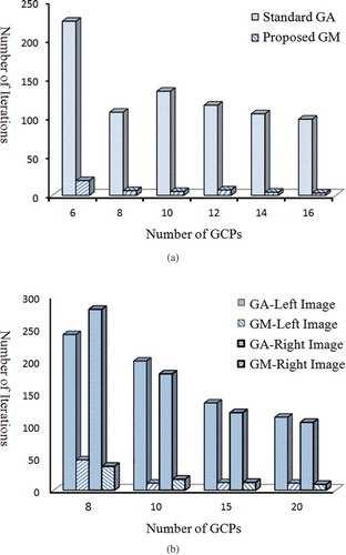
According to the results presented in Tables 2 and 3, the proposed GM algorithm is very time effective. So that its required iterations to complete the optimization process is in average 20 and 11 times less than standard GA, respectively, for Hamedan and Isfahan datasets. Figure 5 represents a graphical comparison between the number of iterations of the standard GA and the proposed GM algorithm.

Figure 5. Comparison between number of iterations of standard GA and proposed GM algorithm: (a) Hamedan dataset, (b) Isfahan dataset (left image), (c) Isfahan dataset (right image).

Accuracies obtained by an optimally structured RFM either by standard GA or the proposed GM algorithm is compared with conventional RFM used in the PCI Geomatica (2003) commercial software package. In this way, the model is estimated with the maximum possible number of parameters corresponding to the similar numbers of GCPs in the latest processes. The obtained results are reported in Table 4, and graphically compared with the results of standard GA and the proposed GM algorithms in Figure 6.

Table 4. Results obtained from conventional RFMs regarding the maximum number of estimable parameters using available GCPs.

		GCPs (in pixels)			ICPs (in pixels)
Image	GCPs, ICPs	RMSE	δr	δc	RMSE	δr	δc	# of coeffs. P1,P2,P3,P4	df
IKONOS	6, 68	3.46	0.58	6.09	9.25	−3.77	9.77	3,2,3,2	2
	8, 66	0.21	−0.02	−0.38	1.84	−1.39	−1.63	4,3,4,3	2
	10, 64	0.18	0.43	0.11	1.34	−1.07	−1.61	5,4,5,4	2
	12, 42	0.29	0.45	−0.37	0.97	−1.01	1.20	6,5,6,5	2
	14, 60	0.16	0.06	0.31	1.34	−1.97	1.86	7,6,7,6	2
	16, 58	0.11	−0.21	−0.13	1.12	1.09	2.39	8,7,8,7	2
SPOT-L	8, 27	0.62	0.95	−0.77	3.74	−3.73	−1.93	4,3,4,3	2
	10, 25	0.47	−0.55	−0.51	2.74	−2.48	2.66	5,4,5,4	2
	15, 20	0.32	0.40	−0.54	2.18	−2.40	−3.19	7,6,7,6	4
	20, 15	0.06	0.16	0.01	6.25	−1.71	19.13	10,9,10,9	2
SPOT-R	8, 27	0.61	0.08	−1.11	4.35	4.08	2.71	4,3,4,3	2
	10, 25	0.60	−0.83	0.73	3.07	3.04	−3.88	5,4,5,4	2
	15, 20	0.40	−0.21	−0.88	2.24	2.83	−3.32	7,6,7,6	4
	20, 15	0.33	1.42	0.17	7.5	−14.46	21.73	10,9,10,9	2

Figure 6. Comparison between accuracies of standard GA and the proposed GM algorithm with traditional RFMs: (a) Hamedan dataset, (b) Isfahan dataset (left and right images).

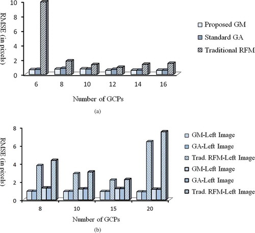
According to the results, upon increasing the number of GCPs, the accuracy of conventional RFMs shows an upward trend and after that comes down. It can be noted that increasing the number of GCPs and consequently the number of estimable parameters cover the under-parameterization problem. However, increasing the number of parameters in the model results in the increment risk of the over-parameterization. Consequently, due to involvement of unnecessary parameters in the model as well as the inherent correlation of some parameters, the overall accuracy of the model will be decreased. Therefore, it seems that conventional RFMs with the maximum number of possible parameters would not be considered as an optimal structure. Then, other structures with less parameters and higher accuracies shall be defined. To survey this issue, with different possible numbers of parameters regarding the same number of GCPs used in Table 4, conventional RFMs applied in IKONOS and SPOT imagery based on a try and error approach. The best results are provided in Table 5.

Table 5. Results obtained from optimal conventional RFMs, surveyed in a try and error approach.

		GCPs (in pixels)			ICPs (in pixels)
Image	GCPs, ICPs	RMSE	δr	δc	RMSE	δr	δc	# of coeffs. P1,P2,P3,P4	df
IKONOS	6, 68	3.46	0.58	6.09	9.25	−3.77	9.77	3,2,3,2	2
	8, 66	0.21	−0.02	−0.38	1.84	−1.39	−1.63	4,3,4,3	2
	10, 64	0.39	0.45	−0.61	1.05	−1.03	−1.04	4,3,4,3	6
	12, 42	0.37	0.57	0.46	0.97	−1.01	−1.20	5,4,5,4	6
	14, 60	0.34	0.73	−0.36	0.81	0.78	1.08	6,5,6,5	6
	16, 58	0.40	−0.48	0.53	0.76	0.77	−0.97	5,4,5,4	14
SPOT-L	8, 27	0.62	0.95	−0.77	3.78	3.73	1.93	4,3,4,3	2
	10, 25	0.66	0.98	0.63	1.92	1.78	1.63	4,3,4,3	6
	15, 20	0.66	0.86	−0.81	1.24	1.39	−1.90	5,4,5,4	12
	20, 15	0.58	0.52	0.94	0.95	1.24	−1.43	6,5,6,5	18
SPOT-R	8, 27	0.61	0.08	−1.11	4.35	−4.08	−2.71	4,3,4,3	2
	10, 25	0.83	−1.22	0.85	2.63	2.71	2.45	4,3,4,3	6
	15, 20	0.66	−0.69	0.97	1.74	−2.60	−2.25	5,4,5,4	12
	20, 15	0.57	0.75	1.10	1.31	2.39	2.29	7,3,7,6	14

As shown in Table 5, the results confirmed the latest discussions about the optimal structure of conventional RFMs. However, fully-parameterized conventional RFMs have the capability to reach precise results, if a sufficient number of well distributed GCPs are available. Accessing numerous numbers of GCPs is hard in most cases; as of the SPOT image used in this research. So, a RFM with less but optimal parameters could be solved precisely with fewer GCPs.

7. Discussion

According to the results shown in Tables 2 and 3, accuracies of both standard GA and proposed GM algorithms are very close to each other. This point is quite expectable due to global searching nature of these algorithms. However, the convergence speed of the proposed GM algorithm is extremely higher than that of standard GA. It should be noted that the convergence speed is just determined with respect to the iterations of algorithms independent from either the technical specifications of the computer processor or coding method of the algorithms. The results are very promising in such a way that the GM algorithm has increased, considerably, the running speed (up to 32 and 18 times for IKONOS and SPOT images respectively). Since, each iteration of algorithm has taken 0.3 second; the whole optimization process is completed in a few seconds. In addition, the proposed GM algorithm benefits from higher degrees of freedom leading to more reliable results in comparison with the standard GA algorithm.

To evaluate the proficiency of the proposed algorithm, conventional RFM is implemented with the maximum possible numbers of parameters considering the similar numbers of GCPs used in standard GA and the proposed GM approaches. The obtained results in Table 4 demonstrate higher accuracies of the proposed GM algorithm while using less parameters in the structure of the model in comparison to the conventional RFMs. This provides the higher degrees of freedom and hence, more reliable results. As another point, the larger number of parameters does not lead always to a higher accuracy. This is because of an increasing correlation between the parameters or over-parameterization problem. In this regard, different possible structures of conventional RFMs are applied in the imagery considering the same number of GCPs in Tables 2 and 3 and the optimal structure of conventional RFMs is recognized for each image through a try and error approach (Table 5). According to the results, it can be inferred that the optimal structure of conventional RFMs would be different for different images. This problem enhances the motivation for using artificial intelligent algorithms for optimization of the RFM structure. Where, investigation of different structures of RFMs is time consuming and low effective. In addition, optimal structures resultant from conventional RFMs is not accurate as the results of artificial intelligent techniques. Because, in conventional RFMs, parameters added just sequentially to the model and not essentially in an optimal approach. Then, there is no possibility to take the advantage of some parameters in the case of using a few numbers of GCPs. Accordingly, there will be the risk of under-parameterization problem and considerable reduction of accuracy. On the other hand, making use of a large number of parameters allows the model to be structured with probably some unnecessary parameters. This will increase the correlation of parameters and may cause to over-parameterization problem which limits again the accuracy of the model.

8. Conclusion

Taking the advantages of an appropriate optimization algorithm for optimal terms selection of a RFM provides the possibility of reducing the number of needed control points and avoiding the over-parameterization problem. GA converges with high possibility to an optimized solution globally, due to its global search in solution space. However, running speed of this algorithm is quite lower than local searching algorithms. To tackle with this problem, a novel optimization algorithm is proposed adopting from the GM concept. This article has examined the proposed GM algorithm in optimal terms selection of a RFM and the results are evaluated with respect to the standard GA and also conventional RFM.

According to the results, the proposed model benefits from less iterations while the accuracy is similar or even better than standard GA. This would be a prominent step to speed up artificial intelligent algorithms for optimization of RFMs structure. Moreover, the proposed algorithm is somehow more accurate than conventional RFMs despite of using fewer parameters. This leads to a higher degree of freedom and more reliable results. One of the limitations of artificially intelligent algorithms is making the use of dependent check points through the optimization process.

The proposed GM algorithm could be considered as a new technique for solving any other optimization problem. So, it would be suggested to examine its performance in solving standard optimization problems.

Disclosure statement

No potential conflict of interest was reported by the authors.

References

- Aguilar, M. A., M. M. Saldana, and F. J. Aguilar. 2013. “Assessing Geometric Accuracy of the Orthorectification Process from Geoeye-1 Andworldview-2 Panchromatic Images.” International Journal of Applied Earth Observation and Geoinformation 21: 427–435. doi:10.1016/j.jag.2012.06.004.
- Chakraborty, U. K., and D. G. Dastidar. 1993. “Using Reliability Analysis to Estimate the Number of Generations to Convergence in Genetic Algorithms.” Information Processing Letters 46: 199–209. doi:10.1016/0020-0190(93)90027-7.
- Davis, T. E., and J. C. Principe. 1993. “A Markov Chain Framework for the Simple Genetic Algorithm.” Evolutionary Computation 1 (3): 269–288. doi:10.1162/evco.1993.1.3.269.
- De Jong, K. A. 1985. “Genetic Algorithms: A 10 Year Perspective.” International conference on Genetic Algorithms, Carnegie-Mellon University, Pittsburgh, PA, July 24–26, 169–177.
- Deltsidis, P., and C. Ioannidis. 2011. “Orthorectification of Worldview-2 Stereo Pair Using a New Rigorous Orientation Model.” International archives of the Photogrammetry, Remote Sensing and Spatial Information Sciences, Volume XXXVIII-4/W19, ISPRS Hannover 2011 Workshop, Hannover, June 14–17.
- Dowman, I., and C. V. Tao. 2002. “An Update on the Use of Rational Functions for Photogrammetric Restitution.” Highlights ISPRS 7 (3): 22–29.
- Fraser, C. S., and H. B. Hanley. 2003. “Bias Compensation in Rational Functions for IKONOS Satellite Imagery.” Photogrammetric Engineering & Remote Sensing 69 (1): 53–57. doi:10.14358/PERS.69.1.53.
- Gil, M. L., M. Arza, J. Ortiz, and A. Ávila. 2014. “DEM Shading Method for Thecorrection of Pseudoscopic Effect on Multi-Platform Satellite Imagery.” GIScience & Remote Sensing 51 (6): 630–643. doi:10.1080/15481603.2014.988433.
- Goldberg, D. E. 1989. Genetic Algorithms in Search, Optimization, and Machine Learning. Boston, MA: Addison-Wesley.
- Greve, C. W., C. W. Molander, and D. K. Gordon. 1992. “Image Processing on Open Systems.” Photogrammetric Engineering & Remote Sensing 58 (1): 85–89.
- Gugan, D. 1986. “Practical Aspects of Topographic Mapping from SPOT Imagery.” The Photogrammetric Record 12 (69): 349–355. doi:10.1111/j.1477-9730.1987.tb00581.x.
- Guichard, H. 1983. “Etude Theorique De La Precision Dans L’exploitation Cartographique D’une Satellite a Defilement: Application a SPOT.” Bulletin De La Societe Francaise De Photogrammetrie Et De Teledetection 90: 15–26.
- Gupta, R., and R. I. Hartley. 1997. “Linear Pushbroom Cameras.” IEEE Transactions on Pattern Analysis and Machine Intelligence 19 (9): 963–975. doi:10.1109/34.615446.
- Habib, A. F., M. Morgan, S. Jeong, and K.-O. Kim. 2005. “Epipolar Geometry of Line Cameras Moving with Constant Velocity and Attitude.” ETRI Journal 27: 172–180. doi:10.4218/etrij.05.0104.0086.
- Holland, J. H. 1975. Adaptation in Natural and Artificial Systems. Ann Arbor: University of Michigan Press.
- Kim, T. 2000. “A Study on the Epipolarity of Linear Pushbroom Images.” Photogrammetric Engineering & Remote Sensing 66 (8): 961–966.
- Kratky, V. 1987. “Rigorous Stereophotogrammetric Treatment of SPOT Images.” In SPOT 1-Utilisation Des Images, Bilans, Resultats, edited by CNES, 1195–1204, Paris: CNES.
- Long, T., W. Jiao, and G. He. 2014. “Nested Regression Based Optimal Selection (NRBOS) of Rational Polynomial Coefficients.” Photogrammetric Engineering & Remote Sensing 80 (3): 261–269. doi:10.14358/PERS.80.3.261.
- Long, T., W. Jiao, and G. He. 2015. “RPC Estimation via L1-Norm-Regularized Least Squares (L1LS).” IEEE Transactions on Geoscience and Remote Sensing 53 (8): 4554–4567. doi:10.1109/TGRS.2015.2401602.
- McGlone, C. 1996. “Sensor Modeling in Image Registration. Digital Photogrammetry.” American Society for Photogrammetry and Remote Sensing Bethesda, MD 247: 115–123.
- Muehlenbein, H., and U. K. Chakraborty. 1997. “Gene Pool Recombination Genetic Algorithm and the One Max Function.” Journal of Computing and Information Technology 5 (3): 167–182.
- OGC (Open GIS Consortium). 1999. “The Open GIS Abstract Specification – Topic 7: Earth Imagery.” pdf accessed on 9 December 2007. http://www.opengis.org/docs/99-107.pdf
- Orun, A. B., and K. Natarajan. 1994. “A Modified Bundle Adjustment Software for SPOT Imagery and Photography: Tradeoff.” Photogrammetric Engineering and Remote Sensing 60 (12): 1431–1437.
- Paderes, F. C., E. M. Mikhail, and J. A. Fagerman. 1989. “Batch and On-Line Evaluation of Stereo SPOT Imagery.” Proceedings of the ASPRS-ACSM Convention, Baltimore, MD, April 2–7, 31–40. ASPRS.
- PCI Geomatica. 2003. “PCI Geomatica OrthoEngine User Guide.” Accessed September 5, 2014 https://www.ucalgary.ca/ appinst/doc/geomatica_v91/manuals/orthoeng.pdf
- Radhadevi, P. V., and R. Ramachandran. 1994. “Orbital Attitude Modeling of SPOT Imagery with a Single Ground Control Point.” Photogrammetric Record 14 (84): 973–982. doi:10.1111/j.1477-9730.1994.tb00297.x.
- Robinson, C. 1997. “Genetically Modified Foods and Consumer Choice.” Trends in Food Science & Technology 8: 84–88. doi:10.1016/S0924-2244(97)01019-4.
- Shaker, A., W. Y. Yan, and S. Easa. 2010. “Using Stereo Satellite Imagery for Topographic and Transportation Applications: An Accuracy Assessment.” GIScience & Remote Sensing 47 (3): 321–337. doi:10.2747/1548-1603.47.3.321.
- Tao, C. V., and Y. Hu. 2001. “A Comprehensive Study of the Rational Function Model Photogrammetric Processing.” Photogramm Engineering Remote Sens 67 (12): 1347–1357.
- Tao, C. V., and Y. Hu. 2002. “3D Construction Methods Based on the Rational Function Model Photogrammetric Processing.” Photogramm Engineering Remote Sens 68 (7): 705–714.
- Teo, T. 2011. “Bias Compensation in a Rigorous Sensor Model and Rational Function Model for High-Resolution Satellite Images.” Photogrammetric Engineering & Remote Sensing 77 (12): 1211–1220. doi:10.14358/PERS.77.12.1211.
- Toutin, T. 1986. “Etude Mathematique Pour La Rectification D’images SPOT.” 18e Congres De La Federation Internationale Des Geometres, Canada 1: 379–395.
- Toutin, T. 2006. “Comparison of 3D Physical and Empirical Models for Generating DSMs from Stereo HR Images.” Photogrammetric Engineering & Remote Sensing 72 (5): 597–604. doi:10.14358/PERS.72.5.597.
- Toutin, T., and P. Cheng. 2000. “Demystification of IKONOS.” Earth Observation Magazine (EOM) 9 (7): 17–21.
- Unger, D. R., D. L. Kulhavy, and I. K. Hung. 2013. “Validating the Geometric Accuracy of High Spatial Resolution Multispectral Satellite Data.” GIScience and Remote Sensing 50 (3): 271–280.
- Valadan Zoej, M. J. 1997. “Mathematical Modelling and Geometric Accuracy Testing of MOMS-02 Imagery.” 4th Conference on Geographic Information systems, Tehran, May 3–4.
- Valadan Zoej, M. J., A. Mansourian, B. Mojaradi, and S. Sadeghian. 2002. “2D Georeferencing of Ikonos Imagery Using Genetic Algorithms.” Symposium on Geospatial Theory, Processing and Applications, Ottawa, ON, July 9–12, not paginated CD-ROM.
- Valadan Zoej, M. J., M. Mokhtarzadeh, A. Mansourian, H. Ebadi, and S. Sadeghian. 2007. “Rational Function Optimization Using Genetic Algorithms.” International Journal of Applied Earth Observation and Geoinformation 9 (4): 403–413. doi:10.1016/j.jag.2007.02.002.
- Valadan Zoej, M. J., and G. Petrie. 1998. “Mathematical Modelling and Accuracy Testing of Spot Level 1B Stereopairs.” The Photogrammetric Record 16 (91): 67–82. doi:10.1111/phor.1998.16.issue-91.
- Valadan Zoej, M. J., and S. Sadeghian. 2003. “Orbital Parameter Modeling Accuracy Testing of Ikonos Geo Image.” Photogramm Journal Finland 18 (2): 70–80.
- Westin, T. 1990. “Precision Rectification of SPOT Imagery.” Photogrammetric Engineering and Remote Sensing 56 (2): 247–253.
- Yavari, S., M. J. Valadan Zoej, A. Mohammadzadeh, and M. Mokhtarzade. 2012. “Particle Swarm Optimization of RFM for Georeferencing of Satellite Images.” IEEE Geoscience and Remote Sensing Letters 10 (1): 135–139. doi:10.1109/LGRS.2012.2195153.
- Zhang, L., X. He, T. Balz, X. Wei, and M. Liao. 2011. “Rational Function Modeling for Spaceborne SAR Datasets.” ISPRS Journal of Photogrammetry and Remote Sensing 66: 133–145. doi:10.1016/j.isprsjprs.2010.10.007.