A parametric method for estimation of leaf area index using landsat ETM+ data

Abstract

Leaf Area Index (LAI) is a key variable for monitoring biophysical and biochemical characteristic of vegetation. So far, various remote-sensing methods are proposed to assess this index; each has its own advantages and limitations. In this study, the Scatterplot of NIR and Red bands (SNIR-R) of ETM+ images was used for LAI estimation. For this, nine different parameters consisting of five distances and four angles were extracted from SNIR-R. All possible combinations of these nine parameters were taken into account and as a result, 511 different regression equations were developed for estimation of LAI. The best regression equation (5P-LAI3) was made of two angles and three distances had the highest correlation coefficient (R) of 0.94 and root mean square (RMSE) of 0.75. On another approach, the triangle of scattered data in the SNIR-R was divided into three separate regions based on PVI (Perpendicular Vegetation Index) values. Three different regression equations were fitted to each region. Use of this Triangle Segmentation Model (TSM) improved the results slightly; that is, comparing with the results of general model 5P-LAI3, RMSE reduced to 0.66 and R increased to 0.96. The data collected throughout BigFoot project was used in this study. Comparing with other models in which BigFoot data were used, it was concluded that despite the simplicity of 5P-LAI3 model, it has an acceptable accuracy and TSM showed the highest accuracy, after all.

Keywords:

• remote sensing; vegetation; LAI
• landsat; ETM+

1. Introduction

Leaf area index (LAI) is defined as one-half the total surface area of leaves per unit ground area underneath. There is considerable interest in developing algorithms for estimation of LAI needed in ecological and climatic models (Bonan 1993; Running and Coughlan 1988). Also, LAI is a crucial parameter in calculation of evapotranspiration (Fan et al. 2009), photosynthesis and carbon cycle (Nouvellon et al. 2000), water flows (Cayrol et al. 2000; Plummer et al. 2005), and monitoring greenhouse gases (Plummer et al. 2005).

Due to the importance of LAI, one of the goals in remote sensing is the accurate estimation of this index. All methods for estimation of LAI through satellite images can be classified into three general categories: statistical, physical, and hybrid methods. Strahler (1997), Liang (2005), Propastin and Kappas (2009) have discussed the advantages and limitations of various approaches in LAI estimation.

Statistical models are based on the statistical relationship between LAI and other vegetation indices. In statistical methods, different regression techniques such as Least Square (LS), Reduced Major Axis (RMA), and Canonical Correlation Analysis (CCA) were used by different workers. For instance, Pu (2012) made a comparison between CCA and LS regression techniques for estimation of LAI in the forest through feature extraction. In this method, based on the relationship with LAI, vegetation indices can be divided into two subcategories: multispectral and hyperspectral. In multispectral vegetation indices, usually the red and NIR bands are used where due to the relatively broader bandwidth, the correlation with LAI is not high compared to the indices using hyperspectral bands with narrower bandwidth (Liang 2005). On the other hand, in multispectral subcategory, background soil imposes a noticeable uncertainty (Gardner and Blad 1986). Twele, Erasmi, and Kappas (2008) evaluated the utility of narrowband EO-1 Hyperion and broadband Landsat ETM+ data for the estimation of LAI in a tropical environment. They applied single and multiple spectral bands and spectral indices as predictor variables in RMA and LS regression models. The results showed that prediction ability of most of the regression models were notably higher when applying narrowband data instead of broadband data. In general, statistical methods approach a saturation level when LAI reaches higher values depending on the type of vegetation cover and environmental conditions (e.g. LAI = 6 in Carlson and Ripley 1997) and it is not possible to define a unique relationship between LAI and a specific vegetation index (Liang 2005).

Physical algorithms rely on inverting canopy reflectance models. In these methods, many information about canopy reflectance is needed (Kuusk 1998). So far, different models of this kind have been proposed e.g., SAIL (Scattering by Arbitrarily Inclined Leaves) developed by Verhoef (1984) and MCRM (Markov Chain Reflectance Model) suggested by Kuusk (1995). The main limitation with these methods is their high computational complexity; therefore, they do not have much practical use in global and regional scales. Lookup Tables (LUT) methods are used to solve this problem, but in an ordinary LUT approach, the dimensions of the table have to be large enough to achieve a high degree of accuracy. This may lead to a much slower online search. Moreover, variables such as soil reflectance, leaf reflectance, and transmittance in the canopy have to be known in these tables where these assumptions may considerably reduce the accuracy (Liang 2005).

Hybrid methods combine both statistical and physical models. This may take advantage of the unique features of each method and overcome their shortcomings. The physical part is associated with extensive simulations using canopy reflectance models and the statistical part relies on nonparametric regression techniques to connect vegetation variables to remote-sensing data (Liang 2005). Artificial Neural Network is one of the most popular method among these methods (Da Silva et al. 2014). Hardin and Jensen (2005) applied two different neural network approaches for estimation of urban LAI. The first was trained to detect sites dominated by bare soil using ASTER visible, infrared, and thermal channels. The second estimated LAI as a function of vegetation indices. When the field sample data were introduced to the two networks, the related standard error was 1.25 in LAI units. Menzies et al. (2007) assessed the accuracy of neural network and regression leaf area estimators for the Amazon basin. They reported that the artificial neural network approach is more versatile than traditional statistical techniques in estimation of LAI.

1.1. Definition of soil line

If the reflectance values of all full bare soil pixels with various amounts of moisture are plotted in the Scatterplot of NIR and Red bands (SNIR-R), it can be seen that the points are distributed around a certain line called Soil Line (SL). This line can be characterized by a linear equation of where b and γ are intercept and slope of the SL, respectively. Also ρ_NIR and ρ_red represent the reflectance values in NIR and red bands, respectively. Length, slope, and intercept of the SL are functions of parameters such as soil texture (percent of sand, silt, and clay), soil moisture (dry, moist, saturated), organic matter contents, iron oxide content, and surface roughness (Ångström 1925; Bowers and Hanks 1965).

1.2. Triangle in SNIR-R

In the case where the scene contains both soil and vegetation, the points distribute inside a scatterplot of triangle shape in SNIR-R as shown in Figure 1. According to the amount of vegetation, soil, soil moisture, vegetation species, and even plant growth stage in each pixel, its corresponding point will be placed in a particular position in this scatterplot. Pixels with high NIR and low red reflectance values are populated around the upper vertex of the triangle and represent pixels with dense vegetation cover. The base of this triangle represents the SL connecting water saturated soil (the lower left vertex) to the dry soil (the upper right vertex). Position of each pixel gradually moves away from the SL to the upper vertex of the triangle as the amount of vegetation cover increases (Jensen 2009).

Figure 1. (a) Distribution of reflectance values in SNIR-R. (b) The migration of a single vegetated pixel in SNIR-R during a growing season (Jensen 2009). For full colour versions of the figures in this paper, please see the online version.

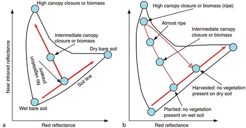
The above-mentioned approaches have their own advantages and disadvantages; therefore, it seems essential to try to improve these methods to achieve more accurate results in estimation of LAI. The purpose of this study is to use the position of each pixel in the SNIR-R made of ETM+ images. It is tried to present a model to estimate LAI using a combination of several parameters including five distances and four angles extracted from the triangle in SNIR-R.

2. Data and methodology

2.1. Data preparation

2.1.1. Study area and in situ measured data

The in situ measured data used in this study are those collected in a validation project of NASA’s Earth Observation System (EOS) called BigFoot. BigFoot collected, archived, and distributed several in situ measurements containing biochemical and biophysical parameters such as LAI, Fraction of Absorbed Photosynthetic Active Radiation (FAPAR), and Net Primary Production (NPP) to validate remote-sensing products. This project was conducted in nine different sites representing various biomes to evaluate the effects of spatial and temporal patterns of ecosystem characteristics on MODIS products. In this study, the data from only five sites have been taken into account mainly because of the lack of access to the rest of BigFoot data. The information regarding these five sites are given in Table 1.

Table 1. The information about five sites of BigFoot campaign (study area).

Site name	Latitude	Longitude	Location	Vegetation type
AGRO	40.00662	−88.29103	Champaign, lllinois	Corn, soybean, fallow
HARV	42.53825	−72.17138	Peter sham, Massachusetts	Eastern hardwood, eastern hemlock, red pine, old field meadow
KONZ	39.08228	−96.56025	Manhattan, Central Kansas	Tall grass Prairie, Short grass Prairie, Shrub community
SEVI	34.3602	−106.7003	Belen, NM, USA	Black gramma, blue gramma
TUND	71.2808	−156.6122	Barrow, AK, USA	Arctic tundra

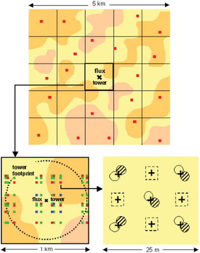
At each site, a 5 × 5 km area was identified using ETM+ imagery. Figure 2 shows the BigFoot field sampling design. Twenty plots of 25 × 25 m each have been placed outside the tower footprint and within a 25-km² grid. These plots will be arranged in a deliberate fashion representing the major cover types (i.e., stratified by cover type). The purpose is to verify that cover-type specific qualities hold over multi-kilometer distances addressing surface features that influence the 25-km² MODIS pixel but not necessarily present within the tower footprint. Eighty plots have been arranged in a systematic spatial cluster near the tower footprint. The purpose of these plots is to allow intensive measurements within the tower footprint and to determine the degree and scale of spatial autocorrelation among cover-type qualities. Plot locations were determined using a real time differential GPS. The accuracy of the system was better than 0.5 m in both the X and Y directions. At each site, LAI was measured at 5–9 subplots per plot using methods described by Gower, Kucharik, and Norman (1999). Then these measured data were averaged to produce a unique value per plot. More information about field data used in this study are listed in Table 2.

Table 2. Information on LAI field measurements.

Site name	Method of measurements	Date of field measurements	Number of LAI measurements	Mean of LAI values
AGRO	Destructive harvest	27 July 1999	34	6.5
		11 September 1999	36	6
		4 July 2000	49	3.3
HARV	Li-Cor LAI-2000	18 June 2000	8	5.2
		27 July 2001, 28 July 2001	30	5.3
		24 August 2002	28	5.7
KONZ	Li-Cor LAI-2000, Destructive harvest	7 June 2000, 8 June 2000	47	2
		25 August 2000, 26 August 2000	50	2
		16 August 2001	58	2.5
SEVI	Destructive harvest	26 July 2002	47	0.3
		22 August 2002	20	0.5
		9 September 2002	49	0.4
		15 November 2002	41	0.4
TUND	Destructive harvest	7 July 2002	42	0.2
			Total = 539

Figure 2. BigFoot field sampling design (+ signs represent points where LAIs are measured).

2.1.2. Satellite image preprocessing

The required satellite images of ETM+ in level 1T were downloaded through the following address: www.earthexplorer.usgs.gov. It is tried to use those images as much as possible close to the date of in situ data collection. Table 3 provides the information about images used in this study.

Table 3. The information about ETM+ images used in this study.

Site name	Date of in situ data collection	Image acquisition date	Difference between image acquisition date and date of in situ data collection (day)
SEVI	26 July 2002	25 July 2002	1
	22 August 2002	19 August 2002	3
	9 September 2002	4 September 2002	5
	15 November 2002	14 November 2002	1
TUND	7 July 2002	18 July 2002	11
KONZ	7 June 2000, 8 June 2000	7 June 2000	0
	25 August 2000,26 August 2000	26 August 2000	0
	16 August 2001	13 August 2001	3
HARV	18 June 2000	23 June 2000	5
	27 July 2001, 28 July 2001	28 July 2001	0
	24 August 2002	23 August 2002	1
AGRO	27 July 1999	29 July 1999	2
	11 September 1999	6 September 1999	5
	4 July 2000	29 June 2000	5
		Total = 14

The study area (5 × 5 km) was extracted from each image and then the Digital Ortho-photo Quadrangles (DOQs) with 1 m pixel size were used to correct ETM+ images geometrically. For this, 20–30 points distributed in the whole scene were used and an average of 0.4 pixel (12 m) RMSE was obtained for each image. Next, a resampling process was carried out to convert 30 m spatial resolution of ETM+ images to 25 m grid.

To carry out the radiometric correction process, first using Fmask algorithm suggested by Zhu and Woodcock (2012), cloud covers, cloud shadows, and water areas were masked. Then, the atmospheric corrections were performed using ENVI/FLAASH (http://www.exelisvis.com/) software where the required parameters were obtained from the images metadata and the data collected in the nearest weather stations to each site. Finally, the images of reflectance values were produced.

2.2. Methodology

Based on the explanation given in Sections 1.1 and 1.2, it is obvious that many information about vegetation and their background soil could be retrieved from the triangle in SNIR-R and these information can be used for estimation of LAI. The method introduced in this study is based on the linear regression of different combinations of nine parameters all extracted from this triangle. These parameters are PVI (Perpendicular Vegetation Index), SR (Simple Ratio), and some other parameters as shown in Figure 3. Point A represents full canopy and Points B and C represent dry soil and wet soil on the SL, respectively.

Figure 3. Nine parameters used for estimation of LAI in this study (four angles and five distances).

The general regression equation is of the form shown in Equation (1) where represents the parameter and is the coefficient weighting parameter .

(1)

First, it is tried to assess LAI using individual and then a combination of these parameters were tested. In this regard, all combinations of these parameters which are 511 different combinations were tested and the best regression equations were introduced.

The SL parameters and the position of Points A, B, and C have to be carefully calculated, because they might affect the results seriously. This will be discussed in the upcoming sections.

2.2.1. Correlation assessment

The correlation between all nine afore-mentioned parameters and the in situ measured values of LAI were investigated. For this, five different forms of regression equations including linear, polynomial (second order), exponential, logarithmic, and power functions were tested. According to Table 4, it can be seen that the second-order polynomial and the linear equation showed the highest correlation, respectively. Although the second-order polynomial showed the best results, however due to the simplification, the linear regression equation was preferred for estimating of LAI.

Table 4. The correlation (R² values) between in situ measured LAI with each of the nine parameters, using linear, polynomial (second order), exponential, logarithmic, and power equations.

Parameter\R^2	linear	Polynomial (second order)	Exponential	Logarithmic	Power
SR	0.83	0.85	0.57	0.80	0.72
PVI	0.82	0.85	0.73	0.52	0.60
	0.83	0.83	0.67	0.62	0.37
	0.07	0.13	0.09	0.08	0.11
	0.73	0.74	0.51	0.67	0.52
	0.51	0.53	0.29	0.53	0.27
α	0.83	0.84	0.70	0.55	0.61
ß	0.55	0.76	0.64	0.37	0.49
Ɣ	0.42	0.53	0.48	0.38	0.47

2.2.2. Soil line determination

The length, slope, and intercept of SL could be affected by parameters such as soil texture, soil moisture content, and soil organic matter content (Ångström 1925; Bowers and Hanks 1965). Therefore, it seems impossible to define one SL globally. In most studies, researchers used their own extracted SL equation from satellite images and suggested their own models. However, it should be considered that these SL equations are not necessarily globally valid and consequently could not be applied in other studies. Therefore in this research, it is tried to reduce the uncertainty involved with the position of SL by using of the average of five different soil lines introduced by different researchers for different soil types. The details of these soil lines are given in Table 5. Each of these SLs was obtained for different soil types with different moisture contents and different percentage of organic matters. However, these authors believe that the 5P-LAI3 model can be used in the most soil conditions. Of course, the model could be readjusted for any SLs if the need arises.

Table 5. Information of five soil lines suggested by different workers.

Reference	Soil type	SL equation	Mean SL
Huete, Post, and Jackson (1984)	Gravel, sand, silt, loam	NIR = 1.166*Red + 0.042
Galvão and Vitorello (1998)	Silt, clay, sand	NIR = 1.368*Red – 0.0117
Baret, Jacquemoud, and Hanocq (1993)	Silica sand, peat, clay, pebble	NIR = 1.176*Red + 0.037	NIR = 1.1628*Red + 0.017
Yoshioka et al. (2010)	Silt, clay, sand	NIR = 1.027*Red – 0.0049
Mobasheri and Bidkhan (2013)	Inorganic clay	NIR = 1.0849*Red + 0.0225

2.2.3. Determination of Point A

As the healthy vegetation canopies get denser, their reflectance values in NIR band get higher and the one in red band decrease to the minimum possible value. This is the typical behavior of healthy vegetation canopies. Therefore to define Point A, the position of the pixel with the highest LAI value (LAI = 11.86) and reflectance values of R = 0.023 and NIR = 0.619 was used.

2.2.4. Determination of Point B

As the soil gets drier, its reflectance values at NIR and red bands increase to the maximum values for bare dry soil (Ångström 1925). Therefore to define Point B, reflectance of some dried soils (zero soil moisture content) with various compositions suggested by different researchers were used (Table 6 and Figure 4). According to Figure 4, it can be seen that these points are so scattered where it renders definition of a fixed point impossible. However to overcome this difficulty, based on the information given in Table 6, the soil sample with the highest reflectance value in the red and NIR bands was selected (i.e. 0.4, 0.482).

Table 6. Reflectance information for various dry soils.

Reference	Soil type	Reflectance in Red band	Reflectance in NIR band
Weidong et al. (2002)	Clay(45%),silt fine(17.6%),silt gross(6.2%),sand fine(6.4%),sand gross(5.1%)organic carbon(7.9%),organic matter(15.8%),Fe(3.9%),…	0.0838	0.1295
	Clay(10.8%),silt fine(40.5%),silt gross(34.3%),sand fine(5.7%),sand gross(2.4%)organic carbon(0.7%),organic matter(1.5%),Fe(1%),…	0.4020	0.4823
	Clay(12.9%),silt fine(34.6%),silt gross(25.2%),sand fine(9.5%),sand gross(7.7%)organic carbon(2.9%),organic matter(5.9%),Fe(0.8%),…	0.1829	0.3048
	Clay(24.8%),silt fine(16.2%),silt gross(12.6%),sand fine(13.8%),sand gross(25%)organic carbon(1.6%),organic matter(3.2%),Fe(4.4%),…	0.1829	0.2248
	Clay(43.4%),silt fine(17.8%),silt gross(9.8%),sand fine(10.4%),sand gross(5.5%)organic carbon(3.8%),organic matter(7.5%),Fe(4.1%),…	0.1352	0.1848
	Clay(42.2%),silt fine(24.2%),silt gross(16%),sand fine(6.4%),sand gross(1.4%)organic carbon(0.8%),organic matter(1.6%),Fe(3.6%),…	0.2248	0.2819
	Clay(44.7%),silt fine(15.1%),silt gross(10.1%),sand fine(6%),sand gross(8.3%)organic carbon(1.3%),organic matter(2.7%),Fe(3.7%),…	0.1600	0.2133
	Clay(4.5%),silt fine(4.9%),silt gross(16.8%),sand fine(41%),sand gross(28.9%)organic carbon(0.5%),organic matter(0.9%),Fe(0.6%),…	0.2876	0.3733
Lobell and Asner (2002)	Argic Aridisol	0.1358	0.2056
	Xeric Andisol	0.1055	0.1744
	Ustic Mollisol	0.1082	0.1958
	Aridic Entisol	0.1506	0.2795
Whiting, Li, and Ustin (2004)	Basin, low sodicity	0.2900	0.3357
Bryant et al. (2003)	Light colored, sandy loam Entisol	0.2663	0.3290
	Red-colored clay and iron-rich Aridsol	0.1777	0.2280
	Dark-colored silt/loam Mollisol with approximately5% organic matter	0.2663	0.3290
Nocita et al. (2013)	Loam-loess on red sandstone and Luxembourgish sandstone	0.2098	0.2721
Mobasheri and Bidkhan (2013)	Inorganic clay	0.2480	0.2895

Note: The highlighted models are better than others.

Figure 4. Plots of nine mentioned parameters against in situ measured LAI.

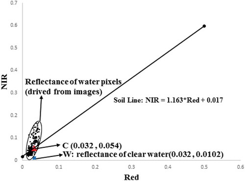
2.2.5. Determination of Point C

As the soil gets moisture, its reflectance values at NIR and red bands decrease to the minimum values for bare wet soil and its behavior approaches to those of water in these bands (Ångström 1925). Point C represents the moistest soil on the SL and its position varies with respect to the percentage of soil moisture content. To find a fixed point as the moistest point, first the reflectance values of few pixels in the deep water regions were retrieved from satellite images used in this study. Then they were plotted in SNIR-R and the intersection of SL with these points selected as Point C. To be more precise, this point represents the soil that is saturated with water where it is completely muddy. This point was nearly equivalent to the position of clean deep water pixel (Point W in Figure 5). The coordinates of C is taken as 0.032, 0.054. Figure 5 illustrates the way of selecting Point C.

Figure 5. Different dry soil positions in SNIR-R and selection of Point B.

However, there might be some uncertainties involved with the selected coordinates of these three points. This issue will be discussed in Section 3.2.

3. Results and discussion

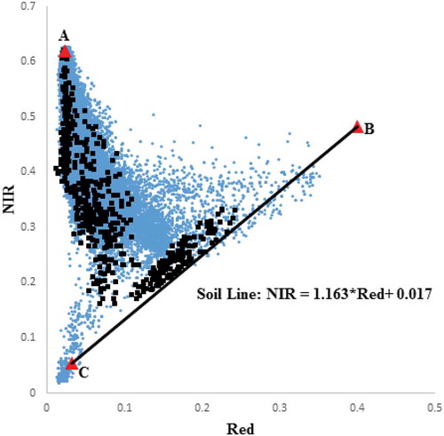
Figure 6 shows scattered pixels in the SNIR-R obtained from Band 3 and Band 4 of ETM+ images used in this study. Also, the SL and three vertices of triangle are indicated. Those pixels where the LAI values are measured, are marked with symbol ■. The measured LAI spans from 0.01 to 12. To achieve a reliable result, the values of LAI used for modelling are populated equally in 0.01–12 range.

Figure 6. The method of choosing Point C.

3.1. A general model for LAI estimation

A set of 404 in situ measured LAI data were selected for modeling and another 135 field data were retained for model evaluation. All linear combinations of nine mentioned parameters, i.e. a total of 511 cases, were considered and a linear regression equation was developed for each of them given by Equation (1). Then using least square method, the coefficients for each of these regression equations were calculated.

To select the best regression equation out of these 511 different combinations, three statistical parameters of R, RMSE, and the percentage of Relative RMSE () were used where the one with the highest correlation and lowest RMSE was taken as the best model. For these 511 regression equations the RMSE, R, and RRMSE values varied between 0.75 and 1.6, between 0.33 and 0.94 and between 29% and 64%, respectively. The information about six of best fits are given in Table 7.

Table 7. The information about six best fits among 511 different combinations of regression equations for estimation of LAI.

Number	Index name	Regression equation	RMSE	RRMSE (%)	R
1	5P-LAI1	Ɣ	0.751	29.87	0.943
2	5P-LAI2	Ɣ	0.752	29.91	0.943
3	5P-LAI3	Ɣ	0.753	29.95	0.943
4	7P-LAI1	Ɣ	0.753	29.95	0.941
5	8P-LAI1	Ɣ	0.753	29.96	0.941
6	5P-LAI4		0.754	29.99	0.943

Note: The highlighted models are better than others.

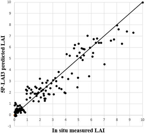
All the equations shown in Table 7 are almost equivalent and have an acceptable accuracy and could be used to estimate LAI. However, 5P-LAI3 is found to be the most simple and versatile model among others. First, because this model is made up of less parameter (five parameters); second, it only depends on two points of A and C plus the SL, and therefore the uncertainty about the position of Point B is not of the concern in this model. In other models, more parameters are used and/or SL plus all three points of A, B, and C are deployed and/or they are less accurate. Figure 7 illustrates the distribution of the field test data versus the 5P-LAI3 predicted LAI values. As can be seen, there is a strong 1:1 relation between measured LAI and model values.

Figure 7. Measured versus 5P-LAI3 model predicted values of LAI. Diagonal is 1:1.

Figure 8 shows the absolute error (calculated from and the percentage of Relative Error (calculated from equation ) or each test data. It can be seen that RE is higher for smaller LAI values and is smaller for higher LAI values. This means that the 5P-LAI3 model is less accurate for LAI values less than one (LAI < 1) in comparison with LAI > 1.

Figure 8. Variation of the absolute error and relative error for different values of LAI test data.

On another approach, it is tried to analyze the effects of variation in the parameters used in 5P-LAI3 on LAI estimation. The results showed that as pixels get closer to SL the accuracy of 5P-LAI3 decreases and vice versa. For instance, as PVI values decrease the accuracy of 5P-LAI3 too decreases.

3.2. Analysis of the effects of position of A, B, and C on 5P-LAI3

The positions of points A, B, and C vary for different vegetation species with different amount of green biomasses, various composition of dry soils, and different percentages of soil moisture content, respectively. To the assess the effects of the position of these three points on the results of 5P-LAI3, their reflectance values in red and NIR bands were gradually increased and decreased for each point.

Since in 5P-LAI3 model Point B is not used, any change in the position of this point has no effect on the results obtained by this model. NIR reflectance value for Point A increased gradually with an interval of 0.01–0.9 and no change were seen in the results. Also, Red and NIR reflectance values for Point C were gradually increased on SL from 0.01 to 0.4 and from 0.02 to 0.48, respectively. The results showed that as Point C gets closer to Point B, the RMSE values for 5P-LAI3 increases (RMSE increased from 0.75 to 0.8 for this variation). It was also found that only variations in the range of 0.02–0.11 for the red band and 0.04–0.145 for the NIR band have no effect on the results.

3.3. Triangle segmentation model (TSM)

Each of the nine afore-mentioned parameters may result in more accurate estimation of LAI in a certain region of the triangle in the SNIR-R compared to the others. As can be seen in Figure 7, the points are almost concentrated in three separate regions where corresponding LAI values are scattered in three intervals of [0–1], [1–4], and [4–12]. For this reason, the triangle in the SNIR-R was divided into three regions according to the range of LAI values and the corresponding range of PVI values. Then, using the data in each region and the method described in Section 3, a different linear regression equation was adopted for each region. Figure 9 shows the three mentioned regions along with the relevant fitted lines and the corresponding statistical parameters. Analysis of these results showed that although the segmentation method has slightly improved the results for LAI < 1 (RMSE decreased from 0.37 to 0.35 and R increased from 0.57 to 0.63), RMSE for this range of LAI values is still considerably high. Nevertheless, it has to be taken into account that according to in situ measured values of LAI at this range, the standard deviation of the field collected data are also higher compared to the standard deviation of LAI in other regions. Furthermore, it is believed that the effects of background soil may impose a noticeable uncertainty to the results, especially in this region. As LAI value increases, the accuracy of the model too increases. For instance, RRMSE for LAI > 4 gets as low as 14%. In addition, all of these new regression equations showed better performance compared to 5P-LAI3 in the corresponding regions.

Figure 9. Three regression equations in three different regions of the triangle in the SNIR-R. Diagonal is 1:1.

Table 8 shows the confusion matrix for the three regression equations in three regions of LAI values. It can be concluded that the average Producer Accuracy (PA) is 97.5%, the average User Accuracy (UA) is 97.3%, and the Overall Accuracy (OA) is 97%. It worth to note that the Overall Accuracy for 5P-LAI3 model was 90%.

Table 8. Confusion matrix for LAI estimation in three classes of values.

		Predicted
		[0–1]	[1–4]	[4–12]	Total	Producer accuracy (%)
True	[0–1]	49	4		53	92.5
	[1–4]		46		46	100
	[4–12]			36	36	100
	Total	49	50	36	135
	User accuracy (%)	100	92	100

Note: The highlighted models are better than others.

Figure 10 shows the whole results of estimated LAI by TSM compared to in situ measured data. According to Figure 10 and based on the results obtained, it can be concluded that TSM has noticeably increased the accuracy; therefore, the overall RMSE is decreased from 0.75 to 0.66, R increased from 0.94 to 0.96, and RRMSE decreased from 29.95% to 25.98%.

Figure 10. The estimated LAI values by TSM against in situ measured data. Diagonal is 1:1.

The effects of variation in the parameters used in TSM on the accuracy of this model was assessed and it was concluded that the satellite-estimated LAI using TSM works well for LAI > 1 and is less accordant with the field-measured data at regions near SL. For instance, as decreases the accuracy of TSM increases.

3.4. Comparison with other models which used BigFoot data

The results obtained by 5P-LAI3, TSM, and other models in which BigFoot data are used are shown in Table 9. It can be seen that the 5P-LAI3 model has an acceptable accuracy as well as simplicity compared to others. It is also obvious that the TSM has the highest accuracy among all other models suggested by the other researchers.

Table 9. Comparison between the models proposed in this study with other models in which the BigFoot data are used.

Reference	Model	R	RMSE
Cohen et al. (2006)	Using the information such as Tasseled Cap index, brightness, greenness, wetness and RMA (Reduced Major Axis) regression for nine site of BigFoot	0.94	0.73
Cohen et al. (2003)	Using the information such as Tasseled Cap index, brightness, greenness, wetness and RMA regression for four site of BigFoot	0.90	0.77
Berterretche et al. (2005)	RMA regression for one site of BigFoot	0.84	1.23
	Anisotropic KED (Kriging with an external drift) regression	0.79	1.44
General model (5P-LAI3)	Ɣ	0.94	0.75
Models proposed by triangle segmentation (TSM)	If PVI = [0–0.11] then: Ɣ Else if PVI = [0.11–0.28] then: Else if PVI > 0.28 then:	0.96	0.66

Note: The highlighted models are better than others.

4. Conclusion

The scatterplot of NIR band against Red band (SNIR-R) in ETM+ images provides many information about vegetation cover and its background soil. Many parameters can be extracted from this scatterplot all usable in LAI estimation. In this study first, nine parameters from the SNIR-R consisting of five distances and four angles were extracted. Then, all possible combinations of these parameters were investigated for LAI assessment. The most simple model with the highest correlation and accuracy was 5P-LAI3 where the values of R = 0.94 and RMSE = 0.75 were achieved. In the second part of this study, considering that each of these nine mentioned parameters may act better in a certain region of the triangle in the SNIR-R compared to the other regions, this triangle was divided into three regions based on PVI values and a separate regression equation was fitted to data in each region. In general, using this TSM resulted in an improvement in the LAI estimation and comparing with the 5P-LAI3 model, RMSE and RRMSE decreased from 0.75 to 0.66 and 30% to 26%, respectively and R increased from 0.94 to 0.96. According to the results, it can be concluded that RRMSE for LAI values less than 1 (LAI < 1) is high (106%) and as LAI increases, the accuracy of the proposed models increases as well. In this study, data collected throughout BigFoot project were used and the results of this study showed considerable improvement in the assessment of LAI values compared to the other models in which the same data were used. It was also concluded that TSM has the highest accuracy among all others.

Disclosure statement

No potential conflict of interest was reported by the authors.

Acknowledgment

We would like to express our profound gratitude to the BigFoot administration and campaign members for their valuable data.

References

- Ångström, A. 1925. “The Albedo of Various Surfaces of Ground.” JSTOR 7: 323–342.
- Baret, F., S. Jacquemoud, and J. F. Hanocq. 1993. “The Soil Line Concept in Remote Sensing.” Remote Sensing Reviews 7 (1): 65–82. doi:10.1080/02757259309532166.
- Berterretche, M., A. T. Hudak, W. B. Cohen, T. K. Maiersperger, S. T. Gower, and J. Dungan. 2005. “Comparison of Regression and Geostatistical Methods for Mapping Leaf Area Index (LAI) with Landsat ETM+ Data over a Boreal Forest.” Remote Sensing of Environment 96 (1): 49–61. doi:10.1016/j.rse.2005.01.014.
- Bonan, G. B. 1993. “Do Biophysics and Physiology Matter in Ecosystem Models?” Climatic Change 24 (4): 281–285. doi:10.1007/BF01091851.
- Bowers, S. A., and R. J. Hanks. 1965. “Reflection of Radiant Energy from Soils.” Soil Science 100 (2): 130–138. doi:10.1097/00010694-196508000-00009.
- Bryant, R., D. Thoma, S. Moran, C. Holifield, D. Goodrich, T. Keefer, and S. Skirvin. 2003. “Evaluation of Hyperspectral, Infrared Temperature and Radar Measurements for Monitoring Surface Soil Moisture.” Proceedings of the First Interagency Conference on Research in the Watersheds, Benson, AZ, October 27–30.
- Carlson, T. N., and D. A. Ripley. 1997. “On the Relation between NDVI, Fractional Vegetation Cover, and Leaf Area Index.” Remote Sensing of Environment 62 (3): 241–252. doi:10.1016/S0034-4257(97)00104-1.
- Cayrol, P., A. Chehbouni, L. Kergoat, G. Dedieu, P. Mordelet, and Y. Nouvellon. 2000. “Grassland Modeling and Monitoring with SPOT-4 VEGETATION Instrument during the 1997–1999 SALSA Experiment.” Agricultural and Forest Meteorology 105 (1–3): 91–115. doi:10.1016/S0168-1923(00)00191-X.
- Cohen, W. B., T. K. Maiersperger, D. P. Turner, W. D. Ritts, D. Pflugmacher, R. E. Kennedy, A. Kirschbaum, S. W. Running, M. Costa, and S. T. Gower. 2006. “MODIS Land Cover and LAI Collection 4 Product Quality across Nine Sites in the Western Hemisphere.” IEEE Transactions on Geoscience and Remote Sensing 44 (7): 1843–1857. doi:10.1109/TGRS.2006.876026.
- Cohen, W. B., T. K. Maiersperger, Z. Yang, S. T. Gower, D. P. Turner, W. D. Ritts, M. Berterretche, and S. W. Running. 2003. “Comparisons of Land Cover and LAI Estimates Derived from ETM+ and MODIS for Four Sites in North America: A Quality Assessment of 2000/2001 Provisional MODIS Products.” Remote Sensing of Environment 88 (3): 233–255. doi:10.1016/j.rse.2003.06.006.
- Da Silva, R. D., L. S. Galvão, J. R. Dos Santos, C. V. De J. Silva, and Y. M. De Moura. 2014. “Spectral/Textural Attributes from ALI/EO-1 for Mapping Primary and Secondary Tropical Forests and Studying the Relationships with Biophysical Parameters.” GIScience & Remote Sensing 51 (6): 677–694. doi:10.1080/15481603.2014.972866.
- Fan, L. Y., Y. Z. Gao, H. Brück, and C. Bernhofer. 2009. “Investigating the Relationship between NDVI and LAI in Semi-Arid Grassland in Inner Mongolia Using In-Situ Measurements.” Theoretical and Applied Climatology 95 (1–2): 151–156. doi:10.1007/s00704-007-0369-2.
- Galvão, L. S., and Í. Vitorello. 1998. “Variability of Laboratory Measured Soil Lines of Soils from Southeastern Brazil.” Remote Sensing of Environment 63 (2): 166–181. doi:10.1016/S0034-4257(97)00135-1.
- Gardner, B. R., and B. L. Blad. 1986. “Evaluation of Spectral Reflectance Models to Estimate Corn Leaf Area while Minimizing the Influence of Soil Background Effects.” Remote Sensing of Environment 20 (2): 183–193. doi:10.1016/0034-4257(86)90022-2.
- Gower, S. T., C. J. Kucharik, and J. M. Norman. 1999. “Direct and Indirect Estimation of Leaf Area Index, Fapar, and Net Primary Production of Terrestrial Ecosystems.” Remote Sensing of Environment 70 (1): 29–51. doi:10.1016/S0034-4257(99)00056-5.
- Hardin, P. J., and R. R. Jensen. 2005. “Neural Network Estimation of Urban Leaf Area Index.” GIScience & Remote Sensing 42 (3): 251–274. doi:10.2747/1548-1603.42.3.251.
- Huete, A. R., D. F. Post, and R. D. Jackson. 1984. “Soil Spectral Effects on 4-Space Vegetation Discrimination.” Remote Sensing of Environment 15 (2): 155–165. doi:10.1016/0034-4257(84)90043-9.
- Jensen, J. R. 2009. Remote Sensing of the Environment: An Earth Resource Perspective 2/e. Upper Saddle River, NJ: Pearson/Prentice Hall.
- Kuusk, A. 1995. “A Markov Chain Model of Canopy Reflectance.” Agricultural and Forest Meteorology 76 (3–4): 221–236. doi:10.1016/0168-1923(94)02216-7.
- Kuusk, A. 1998. “Monitoring of Vegetation Parameters on Large Areas by the Inversion of a Canopy Reflectance Model.” International Journal of Remote Sensing 19 (15): 2893–2905. doi:10.1080/014311698214334.
- Liang, S. 2005. Quantitative Remote Sensing of Land Surfaces. Vol. 30. Hoboken, NJ: John Wiley & Sons.
- Lobell, D. B., and G. P. Asner. 2002. “Moisture Effects on Soil Reflectance.” Soil Science Society of America Journal 66 (3): 722–727.
- Menzies, J., R. Jensen, E. Brondizio, E. Moran, and P. Mausel. 2007. “Accuracy of Neural Network and Regression Leaf Area Estimators for the Amazon Basin.” GIScience & Remote Sensing 44 (1): 82–92. doi:10.2747/1548-1603.44.1.82.
- Mobasheri, M. R., and N. G. Bidkhan. 2013. “Development of New Hyperspectral Angle Index for Estimation of Soil Moisture Using in Situ Spectral Measurments.” ISPRS-International Archives of the Photogrammetry, Remote Sensing and Spatial Information Sciences XL-1/W3 (3): 481–486. doi:10.5194/isprsarchives-XL-1-W3-481-2013.
- Nocita, M., A. Stevens, C. Noon, and B. Van Wesemael. 2013. “Prediction of Soil Organic Carbon for Different Levels of Soil Moisture Using Vis-Nir Spectroscopy.” Geoderma 199: 37–42. doi:10.1016/j.geoderma.2012.07.020.
- Nouvellon, Y., S. Rambal, D. Lo Seen, M. S. Moran, J. P. Lhomme, A. Bégué, A. G. Chehbouni, and Y. Kerr. 2000. “Modelling of Daily Fluxes of Water and Carbon from Shortgrass Steppes.” Agricultural and Forest Meteorology 100 (2–3): 137–153. doi:10.1016/S0168-1923(99)00140-9.
- Plummer, S., O. Arino, F. Fierens, G. Bortstlap, J. Chen, G. Dedieu, and M. Simon. 2005. “The GLOBCARBON Initiative: Multi-Sensor Estimation of Global Biophysical Products for Global Terrestrial Carbon Studies.” MERIS (A) ATSR Workshop 2005, Vol. 597, Frascati, December, 40.
- Propastin, P. A., and M. Kappas. 2009. “Integration of Landsat ETM+ Data with Field Measurements for Mapping Leaf Area Index in the Grasslands of Central Kazakhstan.” GIScience & Remote Sensing 46 (2): 212–231. doi:10.2747/1548-1603.46.2.212.
- Pu, R. 2012. “Comparing Canonical Correlation Analysis with Partial Least Squares Regression in Estimating Forest Leaf Area Index with Multitemporal Landsat TM Imagery.” GIScience & Remote Sensing 49 (1): 92–116. doi:10.2747/1548-1603.49.1.92.
- Running, S. W., and J. C. Coughlan. 1988. “A General Model of Forest Ecosystem Processes for Regional Applications I. Hydrologic Balance, Canopy Gas Exchange and Primary Production Processes.” Ecological Modelling 42 (2): 125–154. doi:10.1016/0304-3800(88)90112-3.
- Strahler, A. H. 1997. “Vegetation Canopy Reflectance Modeling—Recent Developments and Remote Sensing Perspectives.” Remote Sensing Reviews 15 (1–4): 179–194. doi:10.1080/02757259709532337.
- Twele, A., S. Erasmi, and M. Kappas. 2008. “Spatially Explicit Estimation of Leaf Area Index Using EO-1 Hyperion and Landsat ETM+ Data: Implications of Spectral Bandwidth and Shortwave Infrared Data on Prediction Accuracy in a Tropical Montane Environment.” GIScience & Remote Sensing 45 (2): 229–248. doi:10.2747/1548-1603.45.2.229.
- Verhoef, W. 1984. “Light Scattering by Leaf Layers with Application to Canopy Reflectance Modeling: The SAIL Model.” Remote Sensing of Environment 16 (2): 125–141. doi:10.1016/0034-4257(84)90057-9.
- Weidong, L., F. Baret, G. Xingfa, T. Qingxi, Z. Lanfen, and Z. Bing. 2002. “Relating Soil Surface Moisture to Reflectance.” Remote Sensing of Environment 81 (2–3): 238–246. doi:10.1016/S0034-4257(01)00347-9.
- Whiting, M. L., L. Li, and S. L. Ustin. 2004. “Predicting Water Content Using Gaussian Model on Soil Spectra.” Remote Sensing of Environment 89 (4): 535–552. doi:10.1016/j.rse.2003.11.009.
- Yoshioka, H., T. Miura, J. A. Demattê, K. Batchily, and A. R. Huete. 2010. “Soil Line Influences on Two-Band Vegetation Indices and Vegetation Isolines: A Numerical Study.” Remote Sensing 2 (2): 545–561. doi:10.3390/rs2020545.
- Zhu, Z., and C. E. Woodcock. 2012. “Object-Based Cloud and Cloud Shadow Detection in Landsat Imagery.” Remote Sensing of Environment 118: 83–94. doi:10.1016/j.rse.2011.10.028.