Bias corrections of CartoDEM using ICESat-GLAS data in hilly regions

Abstract

There are a number of digital elevation models (DEMs) existing worldwide for studying the topography, estimating elevation differences over time and runoff modeling, soil erosion estimation, and so forth, including vertical changes on glaciers. There are various techniques and instruments/sensors used for surface elevation data collection and for monitoring surface changes. Satellite data-based DEMs have been available at global level during the past two decades. Errors and biases may persist in these elevation data-sets. This may be due to limitations of the techniques, sensor instabilities, bad surveying conditions on the ground, and post-processing artifacts. Elevations derived from Geoscience Laser Altimeter System/Ice, Cloud and land Elevation Satellite (GLAS/ICESat) data are one of the most reliable globally available data. The objective of this study is to present a simple and effective method to compute planimetric offsets in the DEM of hilly terrain using GLAS data and perform necessary corrections for improving the elevation accuracy. A slope-based method has been employed for the co-registration of overlapping elevation surfaces for Chandra and Bhaga basins in the Himalaya. Accuracy assessment has been done by computing standard deviation of offsets, which is an indicator of the variability of error distribution. As a result of bias corrections, the standard deviations have decreased from 10.8 m to 6.0 m and 9.0 m to 7.05 m for Chandra and Bhaga basins, respectively.

Keywords:

• co-registration
• DEM
• CartoDEM
• GLAS

1. Introduction

Topographic surveys have been the traditional source of determining the spatial positioning of any place on the Earth’s surface in three dimensions, i.e. the latitude (Y-coordinates), longitude (X-coordinates), and height (Z-coordinates). Surface topography is normally depicted using contours and spot heights on the topographic maps. The spatial data-sets generated through topographical surveys are discrete in nature, whereas many applications and modeling such as hydrological and soil-erosion modeling, watershed development, infrastructure developments and urban planning, and so forth need continuous elevation surfaces. Thus, digital elevation models (DEMs), representing continuously varying variables such as topography, elevation, slope, aspect, are more useful for the aforementioned applications. Remote sensing-based techniques such as photogrammetry (Ahmed et al. 2007; Yang et al. 2009; Shaker, Yan, and Easa 2010), interferometry (Lin 2008; Yang et al. 2009), radargrammetry, and LiDAR (Zandbergen 2010; Petroselli 2012) have been extensively used to generate DEMs during the past three decades. The accuracies of the globally available DEMs such as Advanced Spaceborne Thermal Spectroradiometer (ASTER) and Shuttle Radar Topography Mission (SRTM) have been assessed and reported by various researchers (Chirico, Malpeli, and Trimble 2012; Gómez et al. 2012; Agrawal et al. 2006). DEMs based on satellite data are reported to be vertically accurate between ±5 m and ±20 m root-mean-square error (RMSE) (Bhakar, Srivastav, and Punia 2010). However, the issue of elevation accuracy of satellite-based DEMs has been one of the major concerns for researchers engaged in research on photogrammetry and remote sensing (Hirano, Welch, and Lang 2003; Rabus et al. 2003; Nikolakopoulos, Kamaratakis, and Chrysoulakis 2006). The errors associated with elevation data-sets include both systematic error, i.e. biases, and the random error. Biases may occur in the elevation data-sets because of sensor instabilities, limitations of the data-processing techniques, poor surveying conditions, and post-processing artifacts. The interaction of terrain and land cover characteristics also influences the accuracy of DEMs (Chirico, Malpeli, and Trimble 2012). Vertical accuracy is also affected by processing, interpolation criteria, and appropriate choice of the parameters for DEM structure such as GRID or TIN (Gosciewski 2013). Some of the studies have used elevation data-sets without correcting for biases (e.g. Rignot, Rivera, and Casassa 2003; Sund et al. 2009; Muskett et al. 2009). These biases may directly affect the DEM accuracy and may lead to erroneous estimates of topographic parameters.

Vertical biases in elevation data-sets may be due to planimetric offsets (x, y directions) or vertical offsets in z-direction or both. Vertical errors due to planimetric offsets are neither constant nor linear. In hilly terrain, planimetric offsets in the DEMs, generated using photogrammetric technique, occur because of variation in pixel size due to sensor viewing geometry in high slope areas (Agrawal et al. 2005). Apparent pixel sizes may vary depending upon the viewing direction and the slope direction of the terrain under consideration. Pixel gets elongated if the viewing direction of the sensor is along the slope and gets shortened when viewing direction is opposite to the slope direction. The apparent pixels also cause visualization problems due to pseudoscopic effects in satellite imagery (Gil et al. 2014). Vertical biases due to planimetric offsets can be rectified using precise geolocated elevation data-sets. Ice, Cloud and land Elevation Satellite/Geoscience Laser Altimeter System (ICESat/GLAS), which has standard planimetric errors of 20 cm (Schutz 2002), can be utilized for rectification of the planimetric offsets by co-registering DEM with it. DEM co-registration involves computation of both translational and rotational components with respect to reference data-sets. Translational elements consist of planimetric (x, y) and vertical (z) biases, while rotational elements consist of three angular parameters along x, y, and z axes. Computation of these six parameters between two elevation data-sets requires feature-based image matching which is possible in raster data-sets only. On the other hand, co-registration of raster (e.g. Cartosat digital elevation model, CartoDEM) and vector data (e.g. GLAS point data) may provide translational elements only. In the present study, local slope analysis-based approach (Streutker, Glenn, and Shrestha 2011) has been applied for co-registration of CartoDEM with ICESat/GLAS. The main advantage of the local slope approach is that it can be applied to different types of elevation data-sets, irrespective of the sensor systems and processing techniques applied (Nuth and Kääb 2011). Thus, a simple and effective universal method has been used in the present work to co-register CartoDEM with ICESat for bias correction.

1.1. Co-registration of DEMs

An initial geometric registration is required for the integration/differencing of overlapping raster DEMs of differing resolutions and accuracies. Registration effectively constitutes a surface-to-surface matching in which horizontal and vertical offsets and rotational parameters between the two DEMs are determined and corrected. Offsets can cause inconsistency and discontinuity among data-sets in the overlapping areas. Van Niel et al. (2008) showed that in DEM integration the matching of elevations is sensitive to even small amounts of misregistration, which they concluded as a source of strong correlation between elevation difference and aspect. The registration process involves determination of horizontal and vertical offsets between overlapping DEMs and this offset computation needs to be carried out either separately or simultaneously. If the computation of horizontal and vertical offsets is done separately it is referred to as 2.5D approach, and if both the offsets are computed simultaneously then it is called as 3D approach.

1.1.1. 2.5D approach

In 2.5D registration, computation and removal of planimetric and vertical offsets are done sequentially. Registration of the two DEMs is carried out using image similarity method. A metric is utilized in this image similarity method to quantify the degree of correspondence between two regions of interest extracted from a reference and the target DEM for registration. Three similarity metrics, namely the cross correlation function (CCF), mutual information (MI), and gradient-based mutual information (GMI), are used for this purpose (Fraser and Ravanbaksh 2012). After implementing horizontal registration, vertical offsets are computed by taking the average of the height differences between the two DEMs.

1.1.2. 3D Approach

In 3D approaches, transformation parameters in x, y, and z directions are estimated in a single step instead of two computational steps described above in 2.5D approach. Following are the two approaches used for the purpose.

1.1.2.1. Slope-based approach

The slope-based approach was primarily developed for LiDAR flightline matching (Streutker, Glenn, and Shrestha 2011). However, this approach has also been applied for the registration of DEMs from different sources as it employs surface slope in the determination of the spatial offset between overlapping elevation model surfaces.

1.1.2.2. Iterative closest point (ICP) algorithm

ICP algorithm aims to determine the transformation parameters, comprising three rotations and three translations, for which the error metric defined via Euclidian distances between the corresponding surface points is a minimum. Given two height models, M as a target and P as a reference DEM, the ICP equation can be written as

$M^{\mathrm{\prime }}=R\cdot M+T$

where R and T denote 3D rotation and translation, respectively, and M′ denotes the transformed DEM. The criterion that must be applied in each iteration centers on the minimum sum of squared distances between M′ and P. The steps of the algorithm are as follows:

1. Matching, in which points in both data-sets are associated using the closest Euclidean distance criterion.

2. Optimization, in which the transformation parameters of translation and rotation are determined via least-squares.

3. Transformation of surface points using the estimated transformation parameters.

This process is iterated until the closest point criterion is satisfied (Fraser and Ravanbaksh 2012).

2. Study site

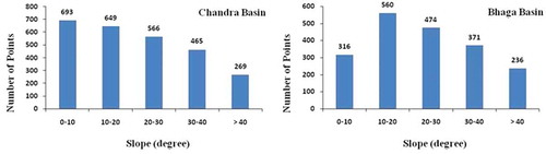
Two sites from the Himalayan region have been chosen for this study. The first site is Chandra basin and the second one is the Bhaga basin. Figure 1 is the location map of the study sites with ICESat paths for available elevation data. ICESat/GLAS points cover various slope categories in the study area, details are given in Figure 2. Both of these basins lie in Chenab subbasin of Indus river basin which has 16,049 glaciers occupying 32,246.43 sq. km of glaciated area (Ajai et al. 2011). Chandra and Bhaga basins fall in the monsoon–arid transition zone. The climate of these basins is mainly characterized by the cold winter extending from October to April.

Figure 1. Showing the location of Chandra and Bhaga basins. For full color versions of the figures in this paper, please see the online version.

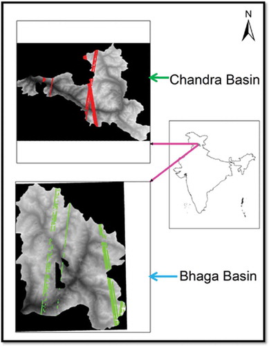
Figure 2. Distribution of GLAS points with slope in Chandra and Bhaga basins.

3. Data used

3.1. ICESat LiDAR profiles

ICESat has a GLAS onboard, designed to collect high precision surface elevations all over the globe. GLAS has been operating for three annual observation campaigns (each of approximately 35 days) since 2003. This instrument combines a 3-cm precision 1064-nm laser altimeter with a laser pointing angle determination system (Sirota et al. 2005) and 1064 and 532-nm cloud and aerosol lidar (Zwally et al. 2002). It uses 1064-nm laser pulses to measure the Earth’s surface. GLAS also measures atmospheric backscatter profiles. The 1064-nm pulses profile the backscatter from thicker clouds, while those at 532 nm use photon-counting detectors and measure the height distributions of optically thin clouds and aerosol layers. A GPS receiver on the spacecraft provides data for determining the spacecraft position, and also the absolute time reference for the instrument measurements and altimetry clock (Abshire et al. 2005). GLAS provides surface elevations with 70 m diameter footprints every 170 m along track. The single shot elevation accuracy is reported to be 15 cm over flat terrain (Zwally et al. 2002), although accuracies better than 5 cm have been achieved under optimal conditions (Fricker et al. 2005). However, ICESat performance degrades over sloping terrain and under conditions of pronounced atmospheric forward scattering and detector saturation. In this study, we have used the GLA06 product between 2003 and 2007 from ICESat data release 428 available from the National Snow and Ice Data Centre (NSIDC) (Zwally et al. 2008).

3.2. Cartosat digital elevation model

Stereoscopic DEMs are generated using photogrammetric principles. Cartosat-1 has a pair of panchromatic cameras having an along track stereoscopic capability to acquire two images simultaneously, one forward looking camera (Fore) at +26° and another rear looking camera (Aft) at −5° with a base-to-height ratio of about 0.63. The spatial resolution is 2.5 m in the horizontal plane and the ground swath is 27 km. DEM derived from Cartosat-1 stereo pair at 10 m spatial resolution was validated (Jayaprasad et al. 2008; Ahmed et al. 2007) and the planimetric and vertical accuracies of the DEM were found to be within 5 m. Indian Space Research Organization has generated CartoDEM for entire India with a spatial resolution of 30 m in public domain, which can be downloaded from NRSC Bhuvan website (bhuvan.nrsc.gov.in). The standard planimetric and vertical accuracies of this DEM are 15 and 8 m, respectively (Muralikrishnan et al. 2011).

4. Methodology

Yu, Tian, and Liu (2004) presented an automatic contour-based 3D terrain matching method to estimate offsets, while Akca (2010) extended the technique of least-squares matching to 3D space as a means of minimizing the weighted sum of squares of offsets between the two surfaces. A similar point-to-point error metric is defined in the ICP method of Besl and McKay (1992). In contrast to the approaches based on least-squares principles to register elevation models, Streutker, Glenn, and Shrestha (2011) introduced a linear method referred to as slope-based approach. This approach for the co-registration of overlapping elevation surfaces is based on local slope analysis. As stated earlier that the terrain plays an important role in controlling the DEM accuracy, broad valleys with gentle slopes yield better accuracy than narrow valleys and steep slopes (Bahuguna, Kulkarni, and Nayak 2008).

Figure 3. Relationship between local slope, coordinate offsets, and the height difference.

4.1. Slope-based approach

The slope-based approach was primarily developed for LiDAR flightline matching. However, this approach has been applied for the registration of DEMs from different sources (Streutker, Glenn, and Shrestha 2011). The local slope plays a vital role in the accuracy of the DEM. The error in the elevation value increases with the increase in the slope value due to the presence of systematic biases. For improving the accuracy of DEM, effect of the local slope needs to be taken into account. The local-slope-based approach is a statistical method based on multiple regression analysis. This regression analysis establishes the relationship between the elevation error and the systematic planimetric offsets in relation to the local slope. The relationship between the local topographic slope m_x, the horizontal and vertical offsets x_offset and h_offset, and the height difference Δh (Figure 3) can be represented as

(1) $\mathrm{\Delta }h=\hspace{0.17em}{h}_{\mathrm{o}\mathrm{f}\mathrm{f}\mathrm{s}\mathrm{e}\mathrm{t}}-\hspace{0.17em}{x}_{\mathrm{o}\mathrm{f}\mathrm{f}\mathrm{s}\mathrm{e}\mathrm{t}}\cdot \hspace{0.17em}{m}_x$(1)

This equation can also be represented in two dimensions as

(2) $\mathrm{\Delta }h=\hspace{0.17em}{h}_{\mathrm{o}\mathrm{f}\mathrm{f}\mathrm{s}\mathrm{e}\mathrm{t}}-\hspace{0.17em}{x}_{\mathrm{o}\mathrm{f}\mathrm{f}\mathrm{s}\mathrm{e}\mathrm{t}}\cdot \hspace{0.17em}{m}_x-\hspace{0.17em}{y}_{\mathrm{o}\mathrm{f}\mathrm{f}\mathrm{s}\mathrm{e}\mathrm{t}}\cdot \hspace{0.17em}{m}_y$(2)

The principal benefit of the slope-based approach is that it predicts the overall 3D offset between two DEMs in a single step through a computationally efficient process. This allows the technique to be applicable to the entire overlap area, in both the x and y dimensions. A random number of points are selected throughout the area of overlap, with the elevation difference and the local slope in x and y calculated at each point. The data are then substituted in Equation 2 to compute x_offset, y_offset, and h_offset.

5. Accuracy assessment

Accuracy assessment of target elevation data-sets is generally carried out by comparing with reference elevation data-sets. The error estimation is carried out using the following two measures of statistics: RMSE and standard deviation (σ). In the present study, accuracy assessment has been carried out by preparing population of residuals (between ICESat as reference and CartoDEM as target) which follow the Gaussian distribution (Equation 3). Subsequently, the parameters such as mean, standard deviation, peak width, and peak height/maximum frequency have been calculated for the above population distribution:

(3) $f(x)=a{e}^{\frac{-{(x-b)}^2}{2c^2}}$(3)

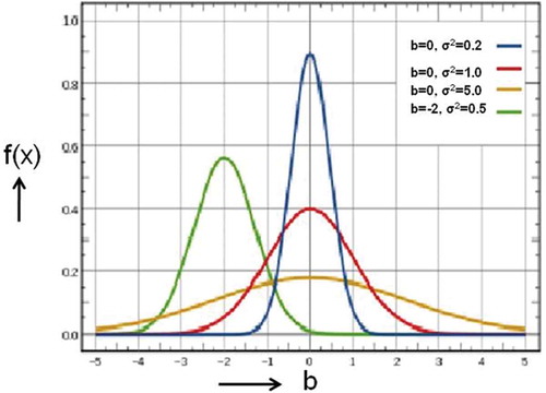
Gaussian parameter a is the height of the curve’s peak, b (mean) is the position of the center of the peak, and c (standard deviation) controls the width of the curve. Error analysis based on Gaussian parameters in pre and post co-registration is performed to observe the effectiveness of the co-registration indicating the level of accuracy.

General plot of Gaussian distribution function is shown in Figure 4 with varying combinations of mean (b) and variance (σ²). The mean value (b), which predicts the peak position of Gaussian function, interprets the positions of blue, red, and yellow curves at b = 0 while peak position of green curve at b = −2. Peak width is described by standard deviation (σ) or variance (σ²). Blue curve which possesses smallest peak width is having smallest value of σ (0.44). As we move towards yellow curve that shows highest peak width, it is having highest value of σ (2.23). Higher the peak width, higher is the error in the data points. It can also be seen that as the peak height increases, peak width decreases, which interprets that data distribution is shifting towards higher accuracy. The above concept/parameters have been used in assessing the errors in the present study.

Figure 4. Gaussian distribution function with varying mean (b) and variance (σ²).

6. Results and discussions

The systematic planimetric and vertical errors present in the DEMs have been removed by the process of co-registration using slope-based approach. The main advantage of the method used in this study is that it predicts the offset between the two data-sets in a single step, making the process computationally efficient due to its statistical nature.

The difference between two elevation data-sets is very sensitive to misregistration for the areas with significant relief. A shift of a fraction of a pixel may cause significant changes in the elevation difference between two elevation data-sets. Townshend et al. (1992) have shown that registration accuracies of 0.2 pixels or less are required to achieve an error of 10%. Dai and Khorram (1998) also showed the impact of misregistration on the accuracy of remotely sensed change detection. They observed that a registration accuracy of less than one-fifth of a pixel is required to attain a change detection error of less than 10% (Dai and Khorram 1998).

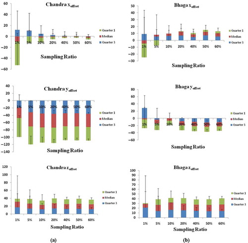
In this study, the local slope approach (discussed in Section 4.1) has been used to compute offsets in x, y, and z directions for CartoDEM using ICESat/GLAS elevation data for Chandra and Bhaga basins. Co-registration parameters (offsets) have been computed using the available ICESat data points as reference (2835 points for Chandra basin and 2160 points for Bhaga basin). In order to study the impact of number of reference points used on the co-registration parameters, an exercise was carried out by randomly choosing 1%, 5%, 10%, 20%, 40%, 50%, and 60% (sampling ratio) of the available ICESat reference points. For each of these sampling ratios, the computations of co-registration parameters were carried out 15 times by taking different random points. To study the impact of sampling ratio on the co-registration parameters, namely maximum/minimum values, difference between maximum and minimum values (range) and standard deviation (σ) were computed for each sampling ratio. The results are provided in Table 1 for Chandra basin and Table 2 for Bhaga basin. It clearly indicates (Tables 1 and 2) that as the sampling ratio increases there is an appreciable reduction in difference and σ of x, y, and z offsets. In Chandra basin, the difference between maximum and minimum values decreases from 92.7 to 8.5 m, 89.8 to 9.2 m, and 25.6 to 1.7 m in x_offset, y_offset, and h_offset, respectively. Standard deviation decreases from 32.3 to 2.5 m, 25.6 to 2.1 m, and 7.8 to 0.5 m in x_offset, y_offset, and h_offset, respectively. In Bhaga basin, the difference between maximum and minimum values decreases from 244.9 to 6.2 m, 100.6 to 7.4 m, and 40.9 to 4.0 m in x_offset, y_offset, and h_offset, respectively. Standard deviation decreases from 52.0 to 1.9 m, 36.0 to 1.8 m, and 13.2 to 0.9 m in x_offset, y_offset, and h_offset, respectively. Reduction in range and σ, in both the basins, clearly indicates that as the sampling ratio increases the variation in x, y and z offsets decreases and it starts stabilizing after the sampling ratio of 20%. Results are also presented graphically in Figure 5 through box plot for each sampling ratio. The results clearly indicate that the range and σ reduce sharply at lower sampling ratios (1–20%) and gently at higher sampling ratios (after 20%) of the available ICESat reference points.

Table 1. Impact of number of random points (sampling ratio) on the co-registration parameters in Chandra basin.

No. of iterations for different sampling rates (Chandra basin)	xoffset (m)			yoffset (m)			hoffset (m)
	Min, Max	Diff.	σ	Min, Max	Diff.	σ	Min, Max	Diff.	σ
1% of total points	−58.2, 34.5	92.7	32.3	−75.8, 13.9	89.8	25.6	0.6, 26.3	25.6	7.8
5% of total points	−22.9, 31.6	54.6	14.8	−58.8, −25.9	32.8	10.6	7.2, 19.6	12.4	3.2
10% of total points	−15.3, 14.8	30.1	8.6	−51.1, −28.0	23.1	6.8	9.2, 16.0	6.7	2.0
20% of total points	−10.4, 10.2	20.6	6.0	−49.0, −24.9	24.0	5.4	9.7, 17.2	7.4	1.8
40% of total points	−6.7, 7.0	13.2	3.4	−43.4, −28.9	14.4	3.5	11.6, 14.9	3.3	0.8
50% of total points	−5.5, 7.7	13.8	3.3	−41.2, −30.7	10.4	2.9	11.3, 14.2	2.9	0.8
60% of total points	−4.6, 3.9	8.5	2.5	−42.1, −32.9	9.2	2.1	11.4, 13.2	1.7	0.5

Table 2. Impact of number of random points (sampling ratio) on the co-registration parameters in Bhaga basin.

No. of iterations for different sampling rates (Bhaga basin)	xoffset (m)			yoffset (m)			hoffset (m)
	Min, Max	Diff.	σ	Min, Max	Diff.	σ	Min, Max	Diff.	Σ
1% of total points	−121.2, 123.6	244.9	52.0	−36.6, 64.0	100.6	36.0	−12.4, 28.5	40.9	13.2
5% of total points	−18.0, 31.5	49.6	13.5	−19.1, 9.4	47.9	12.8	−14.1, 15.3	29.4	7.1
10% of total points	−11.1, 9.9	21.0	5.7	−31.5, 16.3	28.5	8.0	6.0, 24.9	18.8	5.8
20% of total points	−2.3, 9.3	11.6	3.9	−21.7, −0.2	21.4	5.9	7.1, 17.3	10.2	3.0
40% of total points	−2.4, 13.3	15.8	3.5	−17.0, −7.2	9.7	2.7	7.7, 19.8	12.1	3.0
50% of total points	0.6, 8.8	8.2	2.8	17.3, −10.3	6.9	2.0	9.6, 14.4	4.7	1.3
60% of total points	1.4, 7.7	6.2	1.9	−14.9, −7.4	7.4	1.8	10.6, 14.6	4.0	0.9

Figure 5. Box plot for each sampling ratio for Chandra (a) and Bhaga (b) basins.

The computed offsets in the Chandra basin using all the 2835 reference points are found to be −1.6 m and −36.0 m in x and y directions, respectively, while vertical offset is estimated as 12.7 m. The overall estimated planimetric offset is more than a grid size of 30 m for CartoDEM. In the case of Bhaga basin, the offsets estimated in x and y directions are 3.5 m and −11.6 m, respectively, and vertical offset is computed as 13.0 m. The overall planimetric offset is nearly half of a pixel. The above offsets have been corrected for Chandra and Bhaga basins to improve CartoDEM accuracy. Earlier studies have also shown that DEM misregistration is one of the major aspects which need to be considered for enhancing the accuracy of multisource data (Niel et al. 2008; Dai and Khorram 1998). Niel et al. studied the elevation differences between SRTM data and other DEMs. They found that misregistration leads to erroneous elevation difference. The error because of misregistration was greater than or equal to the true difference between the two DEMs for sub-pixel misregistration (Niel et al. 2008).

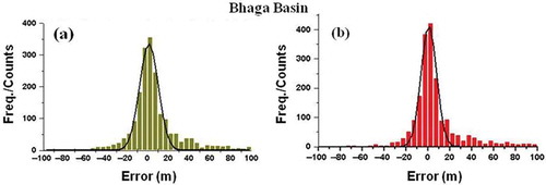
To estimate the effectiveness of co-registration, a statistical analysis has been performed using the method discussed earlier. The histogram of residuals (between elevation data-sets) obtained for Chandra basin, before and after implementing co-registration approach, is fitted to a Gaussian model (Figure 6a and b). Similar analysis has also been carried out for Bhaga basin. The histogram and Gaussian fit for Bhaga basin are given in Figure 7. The Gaussian parameters computed for Chandra and Bhaga basins are given in Table 3.

Table 3. Gaussian parameters before and after bias correction for Chandra and Bhaga basins.

Study area	Mean b (m)	Standard deviation (m)	Width c (m)	Maximum frequency a
Chandra basin
Before correction	1.83	10.8	21.56	394
After correction	1.49	6.0	11.93	699
Bhaga basin
Before correction	1.22	9.0	17.70	334
After correction	0.72	7.05	14.11	413

Figure 6. Vertical error distribution for Chandra basin in original DEM (a) and rectified DEM (b).

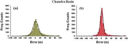
Figure 7. Vertical error distribution for Bhaga basin in original DEM (a) and rectified DEM (b).

It is observed from Figure 6a and b that the maximum frequency/peak height for Chandra basin has increased from 394 to 699 after applying correction. The standard deviation has decreased from 10.8 m to 6.0 m, which indicates the reduction in the peak width and hence the reduction in the overall error distribution. Gaussian width decreases from 21.56 m to 11.93 m indicating the increase in the concentration of data points around the mean value.

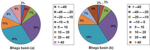
In case of Bhaga basin, standard deviation has decreased from 9.0 m to 7.05 m; Gaussian width has decreased from 17.70 m to 14.11 m and maximum frequency has increased from 334 to 413. Increase in concentration of points along the mean value and reduction in σ have been observed for both the basins as a result of co-registration. As per the statistical approach of Gaussian fit of error distribution, decrement in peak width and increase in peak height represent the improvement in accuracy of the CartoDEM in Chandra and Bhaga basins. The effectiveness of the algorithm has also been assessed by computing percentage distribution of different error classes in pre and post corrections. This has been shown as pie diagram for Chandra basin in Figure 8 and for Bhaga basin in Figure 9. Figure 8 clearly shows that the number of points having the residuals (errors) in the range of ±10 m have increased from 52% to 69% in Chandra basin. The number of points having the residuals of ±20 m has increased from 73% to 85% in Chandra basin. The number of points having residuals greater than ±20 m has reduced from 27% to 15% after corrections in Chandra basin. Figure 9 depicts that the number of points having the residuals (errors) in the range of ±10 m has increased from 56% to 63% in Bhaga basin. The number of points having the residuals of ±20 m has increased from 74% to 79% in Bhaga basin. The number of points having residuals greater than ±20 m has reduced from 26% to 21% after corrections in Bhaga basin. Reduction in points with high errors (residuals) and increase of the points with low errors indicate that high error points have shifted towards the mean value. The above observations clearly indicate the improvement in the accuracy of CartoDEM after the corrections through slope-based approach.

Figure 8. Quantitative representation of vertical error distribution for Chandra basin in original DEM (a) and rectified DEM (b).

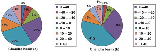
Figure 9. Quantitative representation of vertical error distribution for Bhaga basin in original DEM (a) and rectified DEM (b).

7. Conclusion

Estimation and removal of planimetric offsets and elevation biases are important before any elevation data-sets are put to use. Co-registration between two elevation data-sets is one of the approaches to compute and rectify for such planimetric and vertical offsets. In this study, local slope-based approach has been used for co-registration of CartoDEM using space-borne laser altimeter data-sets (ICESat/GLAS). The results clearly indicate that there is appreciable improvement in the vertical accuracy of the elevation data-set. This method may also be useful in co-registering the global elevation data-sets, such as ASTER and SRTM DEM.

Disclosure statement

We acknowledge that no financial interest or benefit will be raised from the direct applications of our research.

Acknowledgements

We are thankful to Shri. A.S. Kiran Kumar, Director, SAC, for showing interest in this study. We extend our sincere thanks to the National Snow and Ice Data Center for providing ICESat/GLAS data free of cost. We are also thankful to Dr P.K. Pal, DD, EPSA; Dr Prakash Chauhan, Group Head, BPSG; and Dr A.S. Rajawat, Head, GSD for their support.

Additional information

Funding

This work was supported by our own organization, i.e. Space Applications Centre, ISRO.

References

- Abshire, J. B., X. L. Sun, H. Riris, J. M. Sirota, J. F. McGarry, S. Palm, D. H. Yi, and P. Liiva. 2005. “Geoscience Laser Altimeter System (GLAS) on the Icesat Mission: On-Orbit Measurement Performance.” Geophysical Research Letters 32. doi:10.1029/2005GL024028.
- Agrawal, R., P. Jayaprasad, A. Mahtab, S. K. Pathan, and Ajai. 2005. “Effect of IRS 1C/1D Stereo View Angles on the Image Distortions in Hilly Terrains.” MapIndia, Delhi.
- Agrawal, R., A. Mahtab, P. Jayaprasad, S. K. Pathan, and Ajai. 2006. “Validating SRTM Dem with Differential GPS Measurements: A Case Study with Different Terrains.” ISPRS International Symposium on Geospatial Database for Sustainable Development, Goa, September 27–30.
- Ahmed, N., A. Mahtab, R. Agrawal, P. Jayaprasad, S. K. Pathan, Ajai, D. K. Singh, and A. K. Singh. 2007. “Extraction and Validation of Cartosat-1 DEM.” Journal of the Indian Society of Remote Sensing 35 (2): 121–127. doi:10.1007/BF02990776.
- Ajai, S. Nayak, A. V. Kulkarni, A. K. Sharma, I. M. Bahuguna, B. P. Rathore, S. Singh, et al. 2011. Snow and Glaciers of the Himalayas. Ahmedabad: Space Applications Centre (ISRO) . ISBN13 978-81-909978-7-4.
- Akca, D. 2010. “Co-Registration of Surfaces by 3D Least Squares Matching.” Photogrammetric Engineering & Remote Sensing 76 (3): 307–318. doi:10.14358/PERS.76.3.307.
- Bahuguna, I. M., A. V. Kulkarni, and S. Nayak. 2008. “Impact of Slope on DEM Extracted from IRS 1C PAN Stereo Images Covering Himalayan Glaciated Regions: A Few Case Studies.” International Journal of Geoinformatics 4: 2.
- Besl, P. J., and H. D. McKay. 1992. “A Method for Registration of 3-D Shapes.” IEEE Transactions on Pattern Analysis and Machine Intelligence 14 (2): 239–256. doi:10.1109/34.121791.
- Bhakar, R., S. K. Srivastav, and M. Punia. 2010. “Assessment of the Relative Accuracy of ASTER and SRTM Digital Elevation Models along Irrigation Channel Banks of Indira Gandhi Canal Project Area, Rajasthan.” Journal of Water & Land-use Management 10: 1–2.
- Chirico, P. G., K. C. Malpeli, and S. M. Trimble. 2012. “Accuracy Evaluation of an ASTER-Derived Global Digital Elevation Model (GDEM) Version 1 and Version 2 for Two Sites in Western Africa.” GIScience & Remote Sensing 49 (6): 775–801. doi:10.2747/1548-1603.49.6.775.
- Dai, X., and S. Khorram. 1998. “The Effects of Image Misregistration on the Accuracy of Remotely Sensed Change Detection.” IEEE Transactions on Geoscience and Remote Sensing 36: 1566−1577.
- Fraser, C., and M. Ravanbaksh. 2012. Phase 2 - Urban Digital Elevation Modelling in High Priority Regions: Integration of Multi-Resolution Digital Elevation Models, Final Report. Carlton: CRC for Spatial information.
- Fricker, H. A., A. Borsa, B. Minster, C. Carabajal, K. Quinn, and B. Bills. 2005. “Assessment of ICESat Performance at the Salar de Uyuni, Bolivia.” Geophysical Research Letters 32: 1–5, L21S06. doi:10.1029/2005GL023423.
- Gil, M. L., M. Arza, J. Ortiz, and A. Ávila. 2014. “DEM Shading Method for the Correction of Pseudoscopic Effect on Multi-Platform Satellite Imagery.” GIScience & Remote Sensing 51 (6): 630–643. doi:10.1080/15481603.2014.988433.
- Gómez, M. F., J. D. Lencinas, A. Siebert, and G. M. Díaz. 2012. “Accuracy Assessment of ASTER and SRTM DEMs: A Case Study in Andean Patagonia.” GIScience & Remote Sensing 49 (1): 71–91. doi:10.2747/1548-1603.49.1.71.
- Gosciewski, D. 2013. “Selection of Interpolation Parameters Depending on the Location of Measurement Points.” GIScience & Remote Sensing 50 (5): 515–526.
- Hirano, A., R. Welch, and H. Lang. 2003. “Mapping from ASTER Stereo Image Data: DEM Validation and Accuracy Assessment.” ISPRS Journal of Photogrammetry & Remote Sensing 57: 356–370. doi:10.1016/S0924-2716(02)00164-8.
- Jayaprasad, P., R. Agrawal, and S. K. Pathan. 2008. “Utilization Potential of High Resolution Stereo Data for Extracting DEM and Terrain Parameters.” International Archive of Photogrammetry, Remote Sensing and Spatial Information Sciences XXXVII (Part B1): 1117–1122, Beijing.
- Lin, J. 2008. “Ice Surface Topography Digital Elevation Model by Interferometric SAR Method.” GIScience & Remote Sensing 45 (3): 306–329. doi:10.2747/1548-1603.45.3.306.
- Muralikrishnan, S., B. Narender, S. Reddy, and A. Pillai. 2011. Evaluation of Indian National DEM from Cartosat-1 Data. Summary Report (Ver. 1).
- Muskett, R. R., C. S. Lingle, J. M. Sauber, A. S. Post, W. V. Tangborn, B. T. Rabus, and K. A. Echelmeyer. 2009. “Airborne and Spaceborne DEM- and Laser Altimetry-Derived Surface Elevation and Volume Changes of the Bering Glacier System, Alaska, USA, and Yukon, Canada, 1972–2006.” Journal of Glaciology 55: 316–326. doi:10.3189/002214309788608750.
- Niel, T. G. V., T. R. Mc Vicar, L. T. Li, J. C. Gallant, and Q. Yang. 2008. “The Impact of Misregistration on SRTM and DEM Image Differences.” Remote Sensing of Environment 112: 2430–2442. doi:10.1016/j.rse.2007.11.003.
- Nikolakopoulos, K. G., E. K. Kamaratakis, and N. Chrysoulakis. 2006. “SRTM vs ASTER Elevation Products. Comparison for Two Regions in Crete, Greece.” International Journal of Remote Sensing 27 (21): 4819–4838. doi:10.1080/01431160600835853.
- Nuth, C., and A. Kääb. 2011. “Co-Registration and Bias Corrections of Satellite Elevation Datasets for Quantifying Glacier Thickness Change.” The Cryosphere 5: 271–290. doi:10.5194/tc-5-271-2011.
- Petroselli, A. 2012. “LIDAR Data and Hydrological Applications at the Basin Scale.” GIScience & Remote Sensing 49 (1): 139–162. doi:10.2747/1548-1603.49.1.139.
- Rabus, B., M. Eineder, A. Roth, and R. Bamler. 2003. “The Shuttle Radar Topography Mission- a new Class of Digital Elevation Models Acquired by Spaceborne Radar.” ISPRS Journal of Photogrammetry and Remote Sensing 57: 241–262. doi:10.1016/S0924-2716(02)00124-7.
- Rignot, E., A. Rivera, and G. Casassa. 2003. “Contribution of the Patagonia Icefields of South America to Sea Level Rise.” Science 302: 434–437. doi:10.1126/science.1087393.
- Schutz, B. E. 2002. Geoscience Laser Altimeter System Laser Footprint Location (Geolocation) and Surface Profiles. ATBD, Version 3.0, Austin: Center for Space Research, University of Texas.
- Shaker, A., W. Y. Yan, and S. Easa. 2010. “Using Stereo Satellite Imagery for Topographic and Transportation Applications: An Accuracy Assessment.” GIScience & Remote Sensing 47 (3): 321–337. doi:10.2747/1548-1603.47.3.321.
- Sirota, J. M., S. Bae, P. Millar, D. Mostofi, C. Webb, B. Schutz, and S. Luthcke. 2005. “The Transmitter Pointing Determination in the Geoscience Laser Altimeter System.” Geophys Researcher Letters 32: L22S11. doi:10.1029/2005GL024005.
- Streutker, D. R., N. F. Glenn, and R. Shrestha. 2011. “A Slope-Based Method for Matching Elevation Surfaces.” Photogrammetric Engineering & Remote Sensing 77 (7): 743–750. doi:10.14358/PERS.77.7.743.
- Sund, M., T. Eiken, J. O. Hagen, and A. Kääb. 2009. “Svalbard Surge Dynamics Derived from Geometric Changes.” Annals of Glaciology 50: 50–60. doi:10.3189/172756409789624265.
- Townshend, J. R. G., C. O. Justice, C. Gurney, and J. Mc Manus. 1992. “The Impact of Misregistration on Change Detection.” IEEE Transactions on Geoscience and Remote Sensing 30: 1054–1060. doi:10.1109/36.175340.
- Yang, L., L. Jiang, H. Lin, and M. Liao. 2009. “Quantifying Sub-pixel Urban Impervious Surface through Fusion of Optical and InSAR Imagery.” GIScience & Remote Sensing 46 (2): 161–171. doi:10.2747/1548-1603.46.2.161.
- Yu, Q., J. Tian, and J. Liu. 2004. “A Novel Contour-Based 3D Terrain Matching Algorithm Using Wavelet Transform.” Pattern Recognition Letters 25 (1): 87–99. doi:10.1016/j.patrec.2003.09.004.
- Zandbergen, P. A. 2010. “Accuracy Considerations in the Analysis of Depressions in Medium-Resolution Lidar DEMs.” GIScience & Remote Sensing 47 (2): 187–207. doi:10.2747/1548-1603.47.2.187.
- Zwally, H. J., B. Schutz, W. Abdalati, J. Abshire, C. Bentley, A. Brenner, J. Bufton, et al. 2002. “Icesat’s Laser Measurements of Polar Ice, Atmosphere, Ocean, and Land.” Journal of Geodynamics 34: 405–445. doi:10.1016/S0264-3707(02)00042-X.
- Zwally, H. J., R. Schutz, C. Bentley, J. Bufton, T. Herring, B. Minster, J. Spinhirne, and R. Thomas 2008. GLAS/ICESat L1B Global Elevation Data V028, 20 February 2003 to 21 March 2008. Boulder, CO: National Snow and Ice Data Centre Digital media.