Quantifying uncertainty and confusion in land change analyses: a case study from central Mexico using MODIS data

Abstract

Land cover classifications of coarse-resolution data can aid the identification and quantification of natural variability and anthropogenic change at regional scales, but true landscape change can be distorted by misrepresentation of map classes. The Lerma–Chapala–Santiago (LCS) is biophysically diverse and heavily modified by urbanization and agricultural expansion. Land cover maps classified with a Mahalanobis distance algorithm and possibilistic metrics of class membership were used to quantify uncertainty (potential error in class assignment) and change confusion (potential error in land change identification). While land change analysis suggests that ~33% of the landscape underwent a change in class, led by changes from or to the mosaic class (~19% of landscape), classification uncertainty values for 2001 and 2007 were 0.59 and 0.62, respectively, with highest uncertainty among bare soil classes, and an average confusion index value of 0.65, with pixels experiencing change at 0.67 and pixels experiencing persistence at 0.61 on average. These results indicate that uncertainty and potential error in land cover classifications estimates may inhibit accurate assessments of land change. Estimates of land change may be refined using these metrics to more confidently identify true landscape change and to find classes and locations that are contributing to errors in land change assessments.

Keywords:

• land change
• land cover classification
• uncertainty
• MODIS
• Mexico

1. Introduction

Quantifying land cover change is recognized as a grand challenge of remote sensing (Townshend et al. 1991; Cihlar 2000) and, in heterogeneous and rapidly changing landscapes, due to natural fragmented configuration or human influence, there is a need for innovative, systematic monitoring through space and time (Zhang et al. 2003; Treitz and Rogan 2004). The wide variety and magnitude of potential changes in a landscape bring sources of error that introduce uncertainty to classifications of land cover for analyses (Chrisman 1991; Powell et al. 2004). When categorical maps with inherent errors are used for land change analysis, the quantity and location of apparent change in the resulting analysis can be distorted (Pontius 2000), leading many to use continuous soft-classified maps for land change analysis (Hansen et al. 2000; Townshend et al. 2000). Quantitative metrics from continuous soft-classified maps can augment analyses and interpretation of discrete classifications, yielding insight to error sources in land change analyses (Gopal and Woodcock 1994). While it is necessary to identify, quantify, and explain the natural and anthropogenic forces that shape land cover, it is also essential to consider potential errors in these assessments (Lambin et al. 2001; Agarwal et al. 2002). In this study, the quantified potential for error in land cover classifications is referred to as “classification uncertainty” (Chrisman 1991; Eastman 2009), and the compounded effects of classification errors on subsequent change analyses is called “change confusion,” in which changing areas may be mistaken for persistence or vice versa, due to potential errors in one or more of the land cover datasets.

Mexico has a vast, diverse, and rapidly transforming landscape, subject to both natural and anthropogenic forces (West and Augelli 1976; Mas et al. 2002; Alvarez et al. 2003; Klooster 2003) The Lerma–Chapala–Santiago (LCS) watershed in central Mexico epitomizes these characteristics (INE 2003; Cotler, Mazari Hiriart, and de Anda Sanchez 2006) and serves as an ideal case for investigation of uncertainty and confusion in land change analyses. The watershed faces human pressures of urban expansion and agricultural transitions and is subject to perennial seasonal fluctuations, interannual climatic variations, and uncertainties of shifting local and global climates (Aguirre Jimenez and Martinez 2007). The heterogeneous landscape complicates land cover change analyses due to variability both within and between classes and subpixel mixing of thematic classes (Strahler, Woodcock, and Smith 1986; Bradley and Mustard 2005; Iiames, Conglaton, and Lunetta 2013).

By classifying dominant land cover types for 2001 and 2007, this study identifies patterns and sources of error in land cover classification and subsequent change analyses. Data from the Moderate Resolution Imaging Spectroradiometer (MODIS) were classified with a Mahalanobis distance algorithm (Foody et al. 1992) within the Idrisi Taiga geographic information systems package (Eastman 2009) to evaluate sources of error in land change analyses using metrics of classification uncertainty and confusion derived from Mahalanobis typicality values.

In Mexico, investigations of land cover and change have primarily operated at local scales, encompassing a single city and environs (López et al. 2001; Torres-Vera, Prol-Ledesma, and Garcia-Lopez 2009), a state or substate region (Velázquez et al. 2003; Schmook et al. 2011), or assessments of the whole country (Lunetta et al. 2002; Mas et al. 2004). Between these scales lie regional ecosystems and patterns of use that transcend political borders, including mountain ranges, watersheds, coastal floodplains, national parks, and biosphere reserves (Wessels et al. 2004).

2. Land cover monitoring needs and limitations

The ability to monitor changes on the earth’s surface has been facilitated by more than 40 years of research and development of satellite-based remote sensing technologies and applications (Wulder et al. 2008). In order to understand the composition of a landscape and systematically compare landscape conditions over time, there is a perpetual need for comprehensive land cover inventories using remotely sensed data. Thematic land cover maps generated through the discrete classification of satellite imagery have been widely used in the analysis of social and environmental phenomena (Townshend et al. 1991; Cihlar 2000). Global land cover products have achieved great success in the mapping of general land cover types, but these have difficulty distinguishing between distinct land uses that manifest as similar land covers across broad spaces (Friedl et al. 2002; Herold et al. 2008) and have been demonstrated to be inconsistent for many land cover types (Frey and Smith 2007). Further, harmonization and generalization of the different taxonomic schema has proven to be a barrier to the comparison of different land cover products across space and time (Jansen et al. 2006; Herold et al. 2006).

Both producers and users of these categorical land cover products must recognize the inherent limitations for land change analyses, notably:

1. Each pixel in a classified land cover map may be a composite of more than one land cover class, and the frequency of mixed pixels increases as the size of each pixel increases (Strahler, Woodcock, and Smith 1986).

2. Atmospheric conditions or technological calibration may cause variability in the ability of a sensor to consistently represent a landscape over time (Song et al. 2001; Tan et al. 2006).

3. Land cover exemplars used to calibrate land cover classifications may not represent the entire range of variability within a land cover, which can yield inconsistent or misleading results when applied to similar land cover types in new regions (Townshend et al. 2000; Brown, Foody, and Atkinson 2009).

Hence, it is imperative to consider the sources of error and uncertainty inherent to map products and recognize how these impacts propagate through change analyses across broad areas (Goodchild and Gopal 1989).

The spatial resolution of remotely sensed data has an impact on the ability to address potential research questions (Woodcock and Strahler 1987). Coarse-spatial-resolution data from weather satellites, such as the National Oceanic and Atmospheric Administration – advanced very high resolution radiometer (NOAA-AVHRR), with pixels greater than 1 km, have been used to assess regional patterns of vegetation and global land cover characteristics for more than three decades (Justice et al. 1985; Young and Harris 2005). However, the broad extent of each pixel and few spectral channels limit the use of this imagery for the creation of thematic maps of land cover with regional specificity (Loveland et al. 2000; Friedl et al. 2002).

The sensors aboard the Terra and Aqua platforms that comprise the MODIS program record surface characteristics at spatial resolutions of 250–1000 m per pixel, but with spectral properties of Landsat-like multispectral satellites (Wolfe et al. 2002). MODIS data are especially well-suited for regional land cover monitoring due to the broad swath and frequent revisit interval (Borak, Lambin, and Strahler 2000), enabling seamless composite image products (Tan et al. 2006), which can be used to consistently map land cover patterns over broad regions (Friedl et al. 2002). Because classifications based upon regional training signatures have the ability to capture local heterogeneity in a landscape (Schmook et al. 2011), producing these regionally tailored classifications at regular intervals enable identification of patterns and processes at the scale of impact on the landscape (Gustafson and Parker 1992; Turner 1989).

Consideration of the effects of classification errors upon land cover and change analysis has led to a discussion of the uncertainty by many researchers. Gopal and Woodcock (1994), among many others, have described how the composition of landscape features may yield different classification results when these classes are mixed within an arbitrary pixel unit. While methods and standards for cross-comparison of categorical thematic maps were explicated by Congalton (1991), standards for the evaluation of continuous thematic data continue to evolve. Some, including Van der Wel and colleagues (1998) and Goodchild and colleagues (1994), have utilized quantitative metrics for the visualization of uncertainty in classification assessments. Pontius and Cheuk (2006) evaluated and modified existing methods for confusion matrices of continuous data to evaluate land change in heterogeneous landscapes. Foody has extensively addressed both the standards through which accuracy assessments are quantified and tabulated (2008) as well as how they can be compared and evaluated (2009b).

Investigation of the proportion or probability of membership of thematic classes within a coarse-resolution pixel has spawned numerous methods (Leyk, Boesch, and Weibel 2005). Probabilistic methods, such as those derived from maximum-likelihood distributions (Gopal and Woodcock 1994), employ probability density functions to describe the apparent or potential membership of a pixel within a class, which require that the data are normally distributed (Foody 2004). Other methods, such as the use of a classification tree algorithm with boosting, can provide a measure of confidence associated with the class membership of a pixel (McIver and Friedl 2002), which has been related to the likelihood of error in a land cover classification. Probabilistic methods are most appropriate when the legend used for classification uniquely and adequately describes a thematic class appropriate for every pixel in the image (Fisher 1999; Leyk, Boesch, and Weibel 2005).

Possibilistic metrics, such as Mahalanobis typicality values, differ from probabilistic metrics because the resulting metrics need not sum to 1 over all classes (Foody et al. 1992), as the typicality value for each class is calculated independently based on the likelihood of class membership. These typicality values quantify the similarity of a pixel to the set of calibration data that defined each thematic class. As such, if the set of available thematic classes poorly explain a given pixel, the sum of all typicality values may be less than 1, indicating that the signature of a particular pixel is not well-represented by the classes in the legend. If the signature of a pixel might be well-explained by more than one set of class characteristics, the sum of all typicality values for the pixel may be more than 1, indicating redundancy or lack of separation in the class signature definitions. Hence, the set of soft-classified Mahalanobis typicality can yield an indication of the explanatory power of a legend scheme or illustrate sources of class conflation, as described below.

3. Error and uncertainty in land change analyses

For a set of classified land cover maps to be used for land change analyses, they must correctly depict the location and condition of land cover. Error is the inaccurate representation of landscape by the respective land cover map. Two types of error contribute to inaccurate classifications of remotely sensed data, affecting results of single-date land cover inventories and multidate change analyses, by under- or over-estimating the proportions of land cover classes in a landscape (Foody 2009a): errors of location – a land cover class in the wrong geographic position – and errors of attribute – an incorrect thematic class assigned to a particular location.

Location errors may be ascribable to gridding artifacts from data acquisition (Tan et al. 2006) or improper geometric correction (Townshend et al. 1991), for which the metric of positional imprecision of the root mean square error of the distance between a pixel and its true position is commonly used by the remote sensing community (Verbyla and Boles 2000). The geometric accuracy of MODIS imagery is under continual investigation and revision, with a target precision of less than 50 m horizontal deviation per 500 m pixel (Wolfe et al. 2002).

Classifications of heterogeneous or rapidly changing landscapes are susceptible to errors from poor class definition or class conflation (Loveland et al. 1999; Estoque and Murayama 2014). Errors in land cover classification distort the assessment of change across a region, leading to under- or over-estimates in locations that are least typical of the class signatures. There are three major sources of thematic attribute error, given the correct location of a classified pixel on the landscape. First, errors based on composition misrepresent the proportion of land cover categories on the landscape, especially subpixel proportions of land cover classes within moderate/coarse-resolution pixels (Saura 2002). Second, errors based on taxonomy result from a chosen thematic legend scheme with insufficient range and selection of information classes to represent variation across the landscape (Gopal and Woodcock 1994; Brown, Foody, and Atkinson 2009) – if a class definition is too broad, disparate types of land cover may be conflated under a single legend class; if too narrow, a class may not sufficiently include all cases in the study region. Third, errors due to data variance result from insufficient data to distinguish the thematic classes of a given legend (Sabol, Adams, and Smith 1992; Knight 2002), either due to the radiometric resolution of an image, where classes become conflated due to band saturation, or due to an insufficient spectral range or ancillary data chosen for use in the classifier (Rogan and Miller 2006).

When the categorical identification of a given pixel is disputed among more than one thematic class, or when no thematic class in the chosen legend is adequate to describe a pixel, there is uncertainty within the classification. Uncertainty in land cover classifications is a quantitative or qualitative representation of the potential for error within a categorical map (Fritz and See 2008). Classification algorithms that produce sets of continuous soft-classified maps can exhibit cases where the spectral and ancillary data profile of a given pixel may be similarly represented by the thematic definition of more than one legend class. This ambiguity can result from the heterogeneous composition of multiple surface features within a mixed pixel (Woodcock and Strahler 1987), or from the condition of a pixel matching the profiles of data variability of more than one thematic class (Fisher 1999). The classification of a given pixel can also exhibit uncertainty if none of the thematic definitions used for classification adequately explain the pixel, and there is vagueness or lack of knowledge about its identification (Leyk, Boesch, and Weibel 2005). When the soft-classified continuous maps are subjected to mathematical or rule-based decision methods to generate a discrete map of land cover types, pixels that could be explained by more than one thematic class definition or are inadequately explained by any definition in a legend are more likely to be mapped incorrectly (Gopal and Woodcock 1994; McIver and Friedl 2002). When using two or more maps to investigate land change, these “uncertain pixels” can yield spurious transitions due to the inherent potential for error in each map.

4. Study region and selected sample parcels

4.1. The Lerma–Chapala–Santiago watershed

This research was conducted in the LCS watershed of Mexico (19–23.5° N, 99–105.5° W), situated on the southern Central Mesa along the Transverse Neovolcanic Mountain Range (West and Augelli 1976) (Figure 1). Across its 700 km breadth, the LCS spans more than 4000 m in elevation, from the western ridge of the Valley of Mexico to the Pacific Coast, encompassing the drainages of the Lerma River (Río Lerma) (45% of watershed), Lake Chapala, and the Santiago River (Río Grande de Santiago) (55% of watershed), totaling nearly 136,000 km² (de Anda et al. 1998). With diverse geomorphology, the region includes mountain pine–oak forests, mid-elevation shrubby grasslands, and coastal inundated agricultural zones, among other land cover types (West and Augelli 1976). The natural heterogeneity of the region is exemplified by a wide variety of plant species, with the Transvolcanic range and Central Mesa are recognized as centers of pine species diversity (Styles 1993), and the Monarch Butterfly Biosphere Reserve, bordering México state and Michoacán, represents a unique niche critical to the annual cycle of the global population of the species, in spite of widespread illegal logging in the area (Brower et al. 2002).

Figure 1. Study area location of Lerma–Chapala–Santiago (LCS) watershed, with apparent change and persistence, 2001–2007. For full color versions of the figures in this paper, please see the online version.

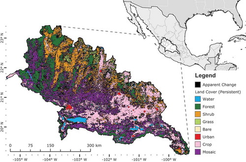
With numerous urban centers (INEGI 2005) and Mexico City just beyond the border, the built environment exerts a strong and constant pressure on natural land cover in this region (López et al. 2001; Alvarez et al. 2003). Urbanization, extensive and intensive agriculture, timber harvesting, and mining fragment the landscape considerably, creating a patchwork of human and natural land covers (Escamilla 1995; Klooster 2003; Cotler, Mazari Hiriart, and de Anda Sanchez 2006). Additionally, this agriculturally intensive region has experienced consolidation of smallholders’ plots into more commercial and mechanized agricultural systems (Sanderson 1986; Appendini and Liverman 1994). The watershed is a major producer of corn, and cultivation of the Agave plant for tequila production has rapidly expanded in recent years, transforming stretches of shrubland and desert to agricultural production, distinct from the maize and grain production common across the rest of the watershed (Dalton 2005).

4.2. Selected sample parcels

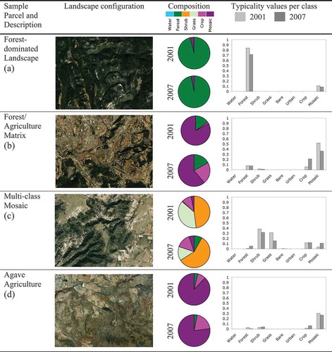
Exemplar parcels representing four distinct land cover compositions were selected within the LCS watershed to serve as case studies, illustrating both common types of landscapes experienced in this region (1 and 2), as well as two examples of landscape compositions that were especially challenging to accurately classify with remotely sensed data.

1. Forest-dominated landscape: Largely undeveloped region on the eastern slope of the Sierra Madre Occidental mountain range near the border of the states of Zacatecas and Jalisco, approximately 2570 m in elevation and dominated by pine forests.

2. Forest/agriculture matrix: Protected zone in the buffer zone of the Monarch Butterfly Biosphere Reserve, 2653 m elevation, with a mix of traditional maize swidden agriculture, cultivated pasture for cattle, and pine forests.

3. Multiclass mosaic: In the northeast LCS, near the border of the states of León and Guanajuato, at an elevation of 2325 m, including forest, shrub, bare soil, grass, and agricultural covers in close proximity, reflecting a matrix of natural and cultivated pastures, with forest and other uses.

4. New agriculture: Outside the city of Guadalajara, near the town of Tequila, Jalisco, approximately 1223 m, with widespread Agave cultivation among natural shrubland and desert.

Four additional zones are described to illustrate regions of high and low confusion index values in regions of both change and persistence identified in the land change analysis (Figure 2).

Figure 2. Confusion index values across the LCS watershed based on Classification Uncertainty Metrics for Land Cover Classifications, 2001–2007.

5. Data and methods

5.1. Field observations

Field observations, including geographic position and estimations of land cover and condition, were collected in January and July 2007 based on an extensive survey of the study region, sampling the navigable road network at an interval of approximately 8–10 km. Locations were recorded with a handheld global positioning system unit (Garmin® GPS60CSx) with an approximate dilution of precision of ±4 m. A systematic set of visual observations of land cover type were estimated based on the 17-class legend system of the International Geosphere–Biosphere Programme (IGBP) at intervals of 30 m, 100 m, and 1 km in the cardinal directions at every sample location, and digital photographs were taken to ensure consistency and enable post-field review. All field-based class estimations, locations, and photographs were integrated into a database of 618 observations used to compile and review calibration and validation data for the analysis.

5.2. Satellite data

Data for the classification included spectral imagery from MODIS MCD43A4 (Justice et al. 2002), collection 5, which is a 16-day image composite produced at a spatial resolution of 500 m/pixel at an interval of 8 days to create a radiometrically consistent, seamless image sequence across the study region for the period 2000–2007 (Schaaf et al. 2002). All MODIS imagery used for this analysis were derived directly from standard image products (Justice et al. 2002), and no additional radiometric corrections were performed. The MCD43A4 product composites 16 days of imagery in association with a bidirectional reflectance distribution function to model image pixel values, providing a single reflectance value for each period normalized to a nadir view (Schaaf et al. 2002). As this methodology requires a minimum number of image views per compositing period, not all pixels can be modeled for every composite image date, resulting in gaps in the continuous data. For this study, any gaps resulting from insufficient data were filled using an annual mean of available nadir-view BRDF-corrected data, per pixel, for each individual spectral band.

The MODIS data volume was reduced using standardized principal components analysis (PCA), calculated with a correlation matrix. Many researchers (Byrne, Crapper, and Mayo 1980; Richards 1984; Ingebritsen and Lyon 1985) have employed PCA in remote analyses as a change analysis procedure to in-paired multispectral imagery sets by correlating component images to spectral information characteristics, such as “overall greenness” or “change in brightness.” Eastman and Fulk (1993) extended the use of standardized PCA to series of AVHRR imagery in Africa, in an effort to relate components to landscape persistence and change. The first component represents a generalized average of the most stable landscape features, and the subsequent components represent the residual variation in the dataset, indicating the most pronounced differences among the image series (Eastman 1993). Eklundh and Singh (1993) compared the use of unstandardized principal components (calculated with a variance/covariance matrix) with standardized principal components (calculated with a correlation matrix) in remote sensing analyses, demonstrating that standardized components markedly improve the signal-to-noise ratio in tested datasets including AVHRR and Landsat.

In this study, standardized PCA was applied to the annual sequence of each spectral band of MODIS imagery. Hence, the annual sequences of 46 dates of 7 spectral bands of MODIS data (322 total images) were reduced to 2 principal component images for each of the 7 spectral bands (14 total images) for each of the two dates. Following Eastman and Fulk (1993), the first principal component image reflects the annual mean of each band and the second component image approximates major annual changes in each band.

5.3. Land cover legend harmonization

A regional legend for classification was prepared to represent the variety of land covers and agricultural land uses in this landscape. Eight thematic classes were selected, based on compatibility with existing land cover products, with the goal of providing a parsimonious definition of visible land covers. In this study, classes have been harmonized to ensure transparency and consistency with existing land cover products and ensure that the products generated will be broadly applicable (Herold et al. 2006).

Existing land cover classification schemes, including those used for products by the International Geosphere–Biosphere Program Data and Information System (IGBP-DIS) DISCover and the Center for Investigations in Environmental Geography (CIGA) at the National Autonomous University of Mexico (UNAM) in Morelia, were considered during both the field data collection and classification. The IGBP DISCover legend contains 17 classes of land covers and land uses, including 11 classes of natural vegetation, 3 classes of developed and mosaic lands, and 3 classes of nonvegetated covers, and has also been used for the existing MODIS MCD12Q1 Land Cover product (Friedl et al. 2002). The INEGI classification (Mas et al. 2002) utilizes a legend based on eight general landscape formation categories.

In the legend for this study, discrete forest type classes have been collapsed into a single “forest” class, as contiguous forest cover occupies relatively little area in the watershed. Similarly, “shrub” and “savanna” classes in the IGBP-DISCover legend have been collapsed into a single “shrub” class to avoid class confusion. Other classes include grassland, urban, barren, water, agriculture, and “mosaic” classes (after the “Cropland and Natural Vegetation Mosaic” of the IGBP-DISCover). Legend class descriptions and comparable land cover classes in the IGBP/MODIS and INEGI legends are summarized in Table 1.

Table 1. Legend scheme and area of land cover classes, 2001 and 2007.

Name	Description	Comparable classes in other legend schemes
		MODIS-IGBP	INEGI-UNAM
Water	Open bodies of water mixed with no other type of cover	Water	Bodies of water
Forest	Cover dominated by broadleaf or needle-leaf trees of at least 10 m in stature	Evergreen needle-leaf forest Evergreen broad-leaf forest Deciduous needle-leaf forest Deciduous broad-leaf forest Mixed forest	Conifer forest Broad-leaf forest Mixed conifer and broad-leaf forest Forest plantation Perennial forest
Shrub	Cover dominated by woody or leafy vegetation less than 10 m in stature	Closed shrublands Open shrublands Woody savannas	Deciduous forest Mesophilic forest Shrub (matorral) Mesquite forest
Grass	Cover dominated by natural or pasture grasses, possibly with interspersed trees or shrubby vegetation	Savannas Grasslands Permanent wetlands	Other vegetation Natural pastures Hydrophilic vegetation
Bare soil	Cover absent of vegetation	Barren or sparsely vegetated	Unvegetated area
Urban	Impermeable built environment	Urban and built-up	Human settlements
Crop	Cover dominated by agricultural products	Croplands	Irrigated agriculture Induced pastures
Mosaic	Cover mixed between agricultural or pasture uses and natural vegetation of any type	Cropland/natural vegetation mosaic	Temporal agriculture

5.4. Calibration data and pseudo-invariant training sites

A combined set of calibration and validation training information was compiled based on comparison of the following reference sources:

1. GPS and photographic field observations (n = 618) in January and July 2007

2. MODIS MCD12Q1v5 Land Cover Product for the years 2001–2005 (Friedl et al. 2002)

3. Mexico National Land Cover Inventory for 2000 (Mas et al. 2002)

4. USGS Global Land Survey Imagery for 2000 and 2005 (Gutman et al. 2008)

In all cases, potential training sites were reviewed for consistency and persistence in an effort to identify features that did not appear to change (pseudo-invariant image features) between the two dates. The selection of pseudo-invariant features has been used widely (De Vries et al. 2007) to ensure radiometric consistency over long time series or among different satellite systems. This study utilizes a calibration database of two-thirds of this set of pseudo-invariant features for the classification of spectral and ancillary imagery (Fortier et al. 2011), reserving an independent one-third for subsequent validation. As such, each image date was trained on the most persistent features between the two dates, in an effort to best identify potential image changes between the two dates. A minimum of 240 exemplar pixels of each class were selected in this combined calibration and validation database, with two-thirds (180 pixels/class) reserved for calibration and one-third (60 pixels/class) for validation.

5.5. Classification typicalities using Mahalanobis distance classifier

To investigate sources of error and uncertainty in the land cover maps, classification of the MODIS data was conducted with a Mahalanobis distance classifier within the Idrisi® Taiga^TM geographic information systems software package (Eastman 2009), using a set of calibration data derived from a randomized two-thirds of the pseudo-invariant image features identified and described above. Mahalanobis distance measures the degree to which the values of a set of explanatory variables at a given location are similar to known examples of that thematic category (Krishnaswamy et al. 2009). This metric is a multivariate equivalent of a Z-score as described in Equation (1):

(1) $D^2=(x-{\mu }_i{)}^t{V}_i^{-1}(x-{\mu }_i)$(1)

where x is the vector of explanatory measures at a location; µ is the vector of the mean explanatory measures for all known instances of a specific land cover type; V⁻¹ is the inverse of the variance/covariance matrix of the explanatory measures for all known instances of the land cover type in question (Foody et al. 1992).

The Mahalanobis distance classifier assumes that the distribution within the thematic classes is normal. If this assumption is fulfilled, a Mahalanobis distance is χ² distributed with degrees of freedom equal k – 1, where k is the number of independent variables (Foody et al. 1992; Eastman 2009). This associated p-value, known as a typicality, is the probability of any location having a Mahalanobis distance greater than or equal to that at an observed location of interest. If, for a given set of data, a pixel has a signature identical to the multivariate centroid of the training sample for that class, the typicality is 1, with values approaching a typicality of 0 at the limits of the distribution (Foody et al. 1992). Although normality of the training sites is considered a prerequisite for a Mahalanobis distance classifier, it has been shown to be robust to mildly skewed distributions (Eastman 2009; Sangermano 2009). The histogram of each spectral image used for classification was plotted and inspected visually, and no distributions exhibited multimodality at either the scale of the watershed or the subset of calibration imagery chosen per class (Figure 3). The Mahalanobis typicality value associated with each land cover class reveals the degree to which a given pixel or collection of pixels are representative of the data on which they were trained. As the data used for training by this analysis were selected to maximize the purity and persistence of land cover types, class typicality indicates the similarity of a pixel or collection of pixels to each persistent land cover class.

Figure 3. Average Mahalanobis typicality values for discrete land cover classes and the entire region.

5.6. Validation of hard-classified land cover maps

Hard-classified land cover maps were validated against an independent subset of one-third of the sample data set from the set of all pseudo-invariant features. Accuracy in the land cover maps was defined as the quantitative agreement of the hard-classified land cover map with an independent set of data using the kappa statistic (Congalton, Oderwald, and Mead 1983). Errors of commission (producer’s accuracy) and omission (user’s accuracy) were also produced for each land cover class in each date (Congalton and Green 2009).

5.7. Classification uncertainty metric

The analysis of possibilistic membership using Mahalanobis typicality values is analogous to the probabilistic membership generated by variants of a maximum-likelihood distribution, except that a set of possibilistic measures are not required to sum to 1.0. Instead, the typicality metric for each land cover class is an independent metric. In the analysis of probabilistic membership values, such a metric can reveal the degree to which classes are conflated or fail to adequately describe a given pixel. An alternative measure for use with possibilistic measures is the measure of classification uncertainty (Eastman 2009), as in the following equation:

(2) $\mathrm{C}\mathrm{l}\mathrm{a}\mathrm{s}\mathrm{s}\mathrm{i}\mathrm{f}\mathrm{i}\mathrm{c}\mathrm{a}\mathrm{t}\mathrm{i}\mathrm{o}\mathrm{n}\mathrm{u}\mathrm{n}\mathrm{c}\mathrm{e}\mathrm{r}\mathrm{t}\mathrm{a}\mathrm{i}\mathrm{n}\mathrm{t}\mathrm{y}=\frac{1-\left(\mathrm{m}\mathrm{a}\mathrm{x}\mathrm{i}\mathrm{m}\mathrm{u}\mathrm{m}-\frac{\mathrm{s}\mathrm{u}\mathrm{m}}{n}\right)}{1-\frac{1}{n}}$(2)

where maximum is highest Mahalanobis typicality value per pixel in a set of images; sum is the sum of all Mahalanobis typicalities in a set of images; n is number of soft-classified thematic class images in a set.

Values range from 0 (representing low classification uncertainty) to 1 (representing high classification uncertainty), and incorporate ambiguity due to class conflation as well as vagueness due to poor class definitions.

5.8. Confusion index of potential land change

In a set of two maps of classification uncertainty there are several cases in which uncertainty in either or both images can contribute to error in the subsequent land change analysis, and the resulting potential for error is referred to as “change confusion.” For example, high values of uncertainty for the same pixel in two maps may indicate that a pixel was improperly classified and change involving that pixel is untrue. High values of uncertainty in only one of two maps may also yield the same type of error. Change involving a pixel with low classification uncertainty values for both dates may yield a result for which there is a decreased chance of error in subsequent land change analysis. The two classification uncertainty maps for 2001 and 2007 were analyzed using the following equation to illustrate potential sources of confusion in change analysis:

(3) $\mathrm{C}\mathrm{o}\mathrm{n}\mathrm{f}\mathrm{u}\mathrm{s}\mathrm{i}\mathrm{o}\mathrm{n}\mathrm{i}\mathrm{n}\mathrm{d}\mathrm{e}\mathrm{x}=\left(\frac{\mathrm{m}\mathrm{a}\mathrm{x}\mathrm{i}\mathrm{m}\mathrm{u}\mathrm{m}+\mathrm{a}\mathrm{v}\mathrm{e}\mathrm{r}\mathrm{a}\mathrm{g}\mathrm{e}}{n}\right)$(3)

where maximum is highest classification uncertainty value per pixel in a set of images; average is the average classification uncertainty value per pixel over a set of images; n is number of classification uncertainty images under comparison.

The confusion index metric was calculated to demonstrate the effects of classification uncertainty in one or both maps used in a categorical land cover change assessment. Potential values range from 0 (representing no confusion in the comparison of the maps) to 1 (representing the highest amount of confusion). By averaging the maximum and average uncertainty values for each pixel, this index can (1) account for two or more dates that have very high uncertainty, resulting in a high confusion index value; (2) account for a pixel that has one date of high uncertainty and one or more of low uncertainty, resulting in a moderately high confusion index value; (3) account for two or more dates that have the same uncertainty, translating this to the comparable confusion index value (whether high or low); (4) identify pixels that have low uncertainty values in all dates, for which there is likely to be little confusion in the resulting change analysis. Additional dates could be compared through this metric, which would increase the value if there were high uncertainty values among one or more of these or decrease the value if there were lower uncertainty values among the added inputs. As this metric was calculated using the above classification uncertainty values for both 2001 and 2007, there is one value per pixel to represent the confusion associated with transitions between the two dates.

5.9. Land change analysis through cross-tabulation of hard-classified maps

Land changes were analyzed through direct comparison of the 2001 and 2007 hard-classified land cover maps, developed through the use of the Mahalanobis distance classifier described already. Maps were directly compared using a cross-tabulation matrix based on the resulting categorical classes (Congalton 1991). Land changes are described as apparent land cover change in Section 6, due to the potential for error in each map used in the change analysis.

5.10. Calculation of typicality, classification uncertainty, and confusion index metrics

Mahalanobis typicality values for each pixel were used to generate metrics of the classification uncertainty for each year and a confusion index, which were compared at different spatial extents to demonstrate the impact of uncertainty on the classification.

Average per-class typicality values were extracted over the entire study area for each date. For a given pixel, the highest typicality value for a class was used to categorically represent that pixel in the hard-classified map. For maps of both dates, extracted Mahalanobis typicality values were averaged for all pixels in which a given class was the dominant land cover in the hard-classified map for each respective date. These per-class typicality values at each spatial extent are tabulated in Table 2.

Table 2. Metrics of classification uncertainty and confusion index for selected sample plots.

Sample	Classification uncertainty, 2001	Classification uncertainty, 2007	Confusion index 2001–2007
Forest-dominated landscape	0.1727	0.2951	0.2797
Forest/agriculture matrix	0.4695	0.5827	0.5876
Multiclass mosaic	0.5460	0.5970	0.6308
Agave agriculture	0.6973	0.7316	0.7700

The average typicality value over the chosen pixels of each class, which can range from 0 to 1, can reveal variability within a land cover class or lack of class separability by a classifier. The average maximum typicality for any class, also ranging from 0 to 1, reveals the similarity of a region to any of the exemplars on which the classifier was calibrated and can serve as an assessment of the thematic legend chosen for classification. Average maximum typicality per pixel can reveal the appropriateness of the legend scheme and training data chosen for classification for two dates. The average sum of typicalities for all classes, which can range from 0 to the total number of classes, can yield an indication of ambiguity or vagueness among class signatures on which the classifier was calibrated.

Metrics of classification uncertainty and confusion index were tabulated based on apparent land cover changes resulting from the differenced hard-classified maps. For each statistic, results were tabulated for the apparent persistent region for each of the eight land cover classes, for the aggregated area of all persistent land cover classes, for the aggregated area of all changing pixels, and for the entire LCS watershed (Table 3).

Table 3. Average metrics of classification uncertainty and confusion index by land cover and transition type across LCS watershed.

Extent of sample	Average classification uncertainty, 2001	Average classification uncertainty, 2007	Average confusion index 2001–2007
All LCS watershed	0.5875	0.5895	0.6457
Persistent
Water	0.4416	0.5233	0.5303
Forest	0.5863	0.6000	0.6547
Shrub	0.5381	0.5391	0.5931
Grass	0.6794	0.6899	0.7426
Bare soil	0.8364	0.8429	0.8773
Urban	0.5588	0.5846	0.6442
Crop	0.4996	0.4659	0.5442
Mosaic	0.5292	0.5422	0.5936
All apparent persistent	0.5502	0.5524	0.6101
All apparent changes	0.6210	0.6229	0.6776

5.11. Extraction typicality, uncertainty, and confusion metrics for select sample parcels

For each of the select sample parcels described in Section 4.2, average classification uncertainty and confusion index metrics were extracted to illustrate the impact of composition on land cover classifications and change analysis. Based on the results of land change analysis and confusion index, four additional examples were selected as representative landscapes demonstrating potential error in land change. These parcels indicate a region experiencing categorical change with a low average confusion index, a region experiencing categorical change with a high average confusion index, persistent land cover with a low average confusion index, and persistent land cover with a high average confusion index. Each parcel was composed of 100 pixels (10 × 10 square of 500 m pixels) in the native MODIS sinusoidal reference framework.

6. Results

6.1. Accuracy of hard-classified land cover maps for 2001 and 2007

The hard-classified land cover map of 2001 had an overall kappa value of 0.90, with per-class kappa values ranging from 0.99 (water), highest, to 0.56 (mosaic), lowest. Per-class accuracy varied widely, with many classes having minimal commission and omission errors, including water (0.05% commission, 4.23% omission), forest (9.86% commission and 2.4% omission), and crop (5.79% omission and 7.22% commission). Several classes occupying small areas had substantial commission errors but minimal omission errors, including bare soil (14.20% commission, 0.00% omission) and urban (11.03% commission, 0.00% omission). Classes exhibiting the highest errors included shrub (23.10% commission, 5.04% omission), grass (19.55% commission, 58.35% omission), and the mosaic class (30.59% commission, 52.10% omission).

The hard-classified land cover map of 2007 had an overall kappa value of 0.91, with per-class kappa values ranging from 0.99 (water), highest, to 0.53 (mosaic), lowest. Per-class accuracy of the 2007 hard-classified map had errors distributed similarly to the 2001 map. Classes with low errors of both commission and omission included water (0.05% commission, 4.51% omission), forest (5.85% commission, 2.13% omission), bare soil (10.06% commission, 1.30% omission), urban (8.80% commission, 0.47% omission), crop (4.89% commission, 10.60% omission). Classes exhibiting higher rates of error included shrub (19.96% commission, 5.65% omission), grass (35.45% commission, 31.40% omission), and mosaic (33.92% commission, 47.99% omission). Full accuracy statistics are presented in Table 4.

Table 4. Accuracy assessment of land cover classifications.

	Water	Forest	Shrub	Grass	Bare soil	Urban	Crop	Mosaic	Errors of commission (%)	Per-class kappa
2001
Water	1926	0	0	0	0	0	1	0	0.05	0.9995
Forest	8	2158	18	2	0	0	3	205	9.86	0.8846
Shrub	5	4	1075	177	0	0	40	97	24.10	0.7203
Grass	1	0	13	177	0	0	14	15	19.55	0.7890
Bare soil	2	0	6	12	145	0	4	0	14.20	0.8578
Urban	31	0	6	2	0	629	39	0	11.03	0.8890
Crop	34	0	1	51	0	0	2506	68	5.79	0.9226
Mosaic	4	41	13	4	0	0	94	354	40.59	0.5565
Errors of omission (%)	4.23	2.04	5.04	58.35	0.00	0.00	7.22	52.10
			Overall accuracy: 89.83%					Overall kappa: 0.8983
2007
Water	1926	0	0	0	0	0	1	0	0.05	0.9995
Forest	17	2254	7	0	0	0	0	116	5.85	0.9294
Shrub	7	8	1119	40	0	1	103	120	19.96	0.7565
Grass	0	0	34	142	2	0	25	17	35.45	0.6322
Bare soil	2	0	1	6	152	0	8	0	10.06	0.8991
Urban	16	0	0	0	0	637	54	0	9.90	0.9004
Crop	46	0	12	12	0	2	2530	58	4.89	0.9314
Mosaic	3	41	13	7	0	0	109	337	33.92	0.5256
Errors of omission (%)	4.51	2.13	5.65	31.40	1.30	0.47	10.60	47.99
			Overall accuracy: 91.11%					Overall kappa: 0.9110

6.2. Land cover change: 2001–2007

6.2.1. Landscape composition in 2001

Based upon the land cover classification of 2001, the landscape was composed of approximately 43% natural classes, including water, forest, shrub, grass, and bare soil covers and 57% anthropogenic classes, including urban, crop, and mosaic classes. The land cover class areas in each product are summarized in Table 5. The order of class proportions is mosaic (31.03%), crop (25.22%), shrub (17.39%), forest (14.61%), grass (7.37%), water (3.60%), urban (0.61%), and bare soil (0.16%).

Table 5. Land cover composition and change by area, 2001–2007.

	Land cover		Land cover change, 2001–2007
Class	2001 Area in km^2 (percent of region)	2007 Area in km^2 (percent of region)	Apparent change 2001–2007 (km^2)	Change as percent of class (%)	Change as percent of region (%)
Water	4832.61	4146.78	−685.83	−14.19	−0.51
	(3.60)	(4.09)
Forest	19,618.08	22,981.14	3363.06	17.14	2.50
	(14.61)	(17.11)
Shrub	23,352.50	24,224.44	871.94	3.73	0.65
	(17.39)	(18.04)
Grass	9901.35	4845.28	−5056.07	−51.06	−3.77
	(7.37)	(3.61)
Bare soil	221.31	376.94	155.63	70.32	0.12
	(0.16)	(0.28)
Urban	823.00	857.99	34.99	4.25	0.03
	(0.61)	(0.64)
Crop	33,870.35	38,588.33	4717.98	13.93	3.51
	(25.22)	(28.74)
Mosaic	41,666.10	38,264.62	−3401.48	−8.16	−2.53
	(31.03)	(28.50)

6.2.2. Landscape composition in 2007

The classified land cover maps of 2007 exhibited similar patterns to the 2001 classified land cover maps, though the order of class proportions varied. Natural covers comprised 42% of the landscape, with anthropogenic classes covering the remaining 58%. The order of class proportions is crop (28.74%), mosaic (28.5%), shrub (18.04%), forest (17.11%), water (4.09%), grass (3.61%), urban (0.64%), and bare soil (0.28%).

6.2.3. Apparent land cover change

Categorical cross-tabulation of the 2001 and 2007 hard-classified land cover maps revealed that 32.76% of the landscape experienced a thematic class transition between the two dates. The per-class apparent land cover change for all classes is listed in Table 5.

The land cover transitions impacting the greatest area are shown in Table 6. Overall, the top 10 land cover transitions represented 82% of the total change. Transitions to or from the mosaic land cover class comprised the top five transitions by area, with pixels shifting both from and to the class from both natural land covers and the crop class.

Table 6. Rank of apparent land cover transitions by impacted area, 2001–2007.

Rank	Transition	Area (km^2)	Percent of LCS (%)
1	Mosaic to forest	5596.15	4.17
2	Mosaic to crop	5165.55	3.85
3	Shrub to mosaic	4119.73	3.07
4	Mosaic to shrub	4047.17	3.01
5	Crop to mosaic	3980.84	2.96
6	Grass to shrub	3158.49	2.35
7	Forest to mosaic	2894.24	2.16
8	Shrub to crop	2567.96	1.91
9	Grass to crop	2489.61	1.85
10	Crop to shrub	1737.02	1.29

6.3. Mahalanobis typicality of land cover classes

6.3.1. Per-class typicality classes across watershed

The average per-class typicality of every pixel across the watershed varied widely.

The bare soil and urban classes, which occupy a small fraction of the landscape, had extremely low typicality of 0.001 and 0.002 in both years. The highest typicality values across the watershed were in the crop and mosaic classes, with average crop typicality values of 0.18 in 2001 and 0.20 in 2007 and average mosaic typicality values of 0.21 in both 2001 and 2007. In both dates, the average maximum typicality over the entire LCS watershed was 0.45. The average sum of typicalities for all classes was 0.697 in 2001, and 0.709 in 2007.

6.3.2. Per-class typicality of persistent land cover

In 2001, the class with the highest average typicality of the persistent pixels on which it was calibrated was the crop class, with a Mahalanobis typicality value of 0.49. Other classes with high average typicality values included shrub (0.48), mosaic (0.44), forest (0.43), grass (0.43), and urban (0.43) classes. Bare soil cover had an average typicality of 0.25, and the water class demonstrated lowest average typicality values, with an average typicality of 0.12 over the pixels that were hard classified as water.

In 2007, shrub cover had the highest average typicality (0.51) of the persistent pixels on which it was calibrated, followed by crop (0.48), grass (0.46), forest (0.43), mosaic (0.43), urban (0.39), bare soil (0.34), and the water (0.12) classes.

6.4. Classification uncertainty for 2001 and 2007

As the classification uncertainty metric is derived from the set of Mahalanobis typicality values generated by the soft classification of each date, there is one classification uncertainty value for each pixel in each date, which was averaged at various scales. In nearly all cases, the classification uncertainty metric for both 2001 and 2007 was very similar. Across the entire watershed, the average classification uncertainty for both dates was 0.59, with the average classification uncertainty of 0.55 for all pixels demonstrating persistence and an average classification uncertainty of 0.62 for any pixel exhibiting a categorical transition between the two dates.

Classification uncertainty values for persistent regions varied among land cover type, with cropland having the lowest classification uncertainty in both dates, with 0.50 in 2001 and 0.47 in 2007. The highest classification uncertainty values were in the bare soil class, with 0.84 in both 2001 and 2007.

6.5. Confusion index between 2001 and 2007 assessments

Across the entire LCS watershed, the average per-pixel confusion index was 0.65, with the average confusion index for pixels demonstrating persistence at 0.61 and the average confusion index for pixels experiencing any categorical change at 0.67. Of pixels demonstrating persistence between 2001 and 2007, the confusion index varied from a low of 0.53 for water to a high of 0.88 for persistent bare soil. The agricultural classes of crop and mosaic that experienced persistence had an average confusion index of 0.54 and 0.59, respectively.

Average classification uncertainty and confusion index values are tabulated in Table 3. Across the entire LCS watershed, the overall average confusion index was 0.65, with an average value of 0.61 for all pixels experiencing persistence between the two dates and an average value of 0.68 for all pixels experiencing a categorical transition between the two dates. The class with the highest confusion index between 2001 and 2007 was bare soil, with a value of 0.88, followed by grass (0.74). All categories had values greater than 0.5, and the class with the lowest confusion index between the two dates was water, with a value of 0.53.

For both changing and persistent pixels between 2001 and 2007, the confusion index varied widely, as illustrated in Figure 4.

Figure 4. Landscape composition and typicality values for select sample parcels.

6.6. Classification and uncertainty in select sample parcels

In the forest-dominated landscape sample, the land cover composition was 96% forest and 4% mosaic in 2001 and 97% forest and 3% mosaic in 2007. The average per-pixel classification uncertainty metric for this parcel was 0.1727 for 2001 and 0.2951 for 2007, yielding a confusion index of 0.2797 for potential change analysis between the two dates.

In the forest/agricultural matrix near the Monarch Butterfly Biosphere Reserve, the land cover composition was 15% forest, 2% crop, and 83% mosaic in the 2001 classification and 17% forest, 22% crop, and 61% mosaic in the 2007 classification. The average per-pixel classification uncertainty metric for this parcel was 0.4595 in 2001 and 0.5827 in 2007, yielding a confusion index of 0.5876 for potential change analysis between the two dates.

In the multiclass mosaic landscape of the northeastern region of the watershed, the land cover composition in 2001 was 48% shrub, 38% grass, 1% bare soil, 10% crop, and 3% mosaic. In 2007, the land cover composition was 8% forest, 58% shrub, 14% grass, 15% crop, and 5% mosaic. The average per-pixel classification uncertainty metric for this parcel was 0.5460 for 2001 and 0.5970 for 2007, yielding a confusion index of 0.6308 for potential change analysis between the two dates.

In the region of expanding Agave agriculture near Tequila, Jalisco, the land cover composition was 4% forest, 8% crop, and 88% mosaic in 2001 and 3% forest, 20% crop, and 77% mosaic in 2007. The average per-pixel classification uncertainty metric for this parcel was 0.6973 for 2001 and 0.7316 for 2007, yielding a confusion index of 0.7700 for potential change analysis between the two dates.

7. Discussion

Regional analyses of land change have the potential to reveal patterns of human activities or natural processes on the landscape. However, the error inherent to the land cover classifications used in change analyses can inhibit accurate assessments of change.

7.1. Regional land cover change analysis

The land change analysis of annual land cover classifications for 2001 and 2007, each mapped at approximately 90% accuracy, suggested that more than 30% of the landscape underwent a change of thematic class during the 7-year period. However, there is reason to suspect that much of this change was attributable to classifier error or changes in landscape condition, rather than a true change in thematic class. For example, the mosaic class was mapped with the lowest per-class kappa in both land cover maps, and yet transitions to and from mosaic land covers represented 6 of the top 10 land apparent land cover transitions between 2001 and 2007 (Table 6). Similarly, the relatively small proportion of the region covered by grass (7.37% in 2001; 3.61% in 2007) and bare soil (0.16% in 2001, 0.28% in 2007) relates to the high proportions of change as a percent of class observed between the two dates and the high classification uncertainty of even persistent regions of these classes (Table 3). The comparison of typicality and classification uncertainty values across even persistent pixels between the two dates indicates that some classes are more difficult to map in this landscape than others using MODIS data. The average maximum typicality per pixel of 0.45 across the entire watershed indicates that while the legend is appropriate for this landscape (e.g., on average, the land cover classes in the resulting maps were typical of the signatures for which they were trained), there are some regions that are more difficult to classify, and landscape composition is a major factor in the performance of classification algorithms.

7.2. Select sample parcels

The analysis of the classification uncertainty and confusion index metrics of the selected sample parcels demonstrates the impact of landscape composition and heterogeneity on the performance of a classifier and the potential for error in land cover classifications. In the forest-dominated landscape, the relative dominance of one land cover type yielded the lowest classification uncertainty metrics for both dates and the lowest confusion index overall. Around the mosaic of agriculture and forest covers near the Monarch Butterfly Biosphere Reserve, the apparent change between the mosaic class and the crop class was demonstrated by an increase in classification uncertainty from 0.4596 in 2001 to 0.5827 in 2007. Although the mosaic class, defined as a mixture of natural and anthropogenic land covers, represents a mixture of the other two classes present in this sample, forest and crop, the apparent change in proportion of these classes generated a confusion index of 0.5876, indicating that change in this region may be a result of error and uncertainty in the classification.

In the heterogeneous multiclass mosaic, high classification uncertainty values of 0.4560 in 2001 and 0.5970 in 2007 can be attributed to ambiguity among potential class definitions, with five different land cover types present in varying proportions in the two land cover maps. Land cover change analysis between these two maps may be susceptible to error due to changes in condition, wherein changes in temperature or precipitation may yield reflectance profiles that cause a pixel of one class to be classified as another.

Vagueness in taxonomic definitions was culpable for the very high classification uncertainty in the new agricultural expansion of Agave in Jalisco state. Because the pixels in this parcel had very low typicality values for all classes, the high confusion index indicates that apparent change in this region is very likely to be attributable to classification error of heterogeneous and variable landscapes rather than true land cover change.

7.3. Extracted change confusion examples

The variability of confusion index values for both changing and persistent pixels between the two dates can give an indication of the reliability of the apparent land change. If a pixel experiencing either change or persistence between the two dates had a low confusion index (closer to 0), there is greater confidence that the transition exhibited in the change analysis represents the true state of the landscape. For pixels experiencing either change or persistence and a high confusion index (closer to 1), this apparent change may either represent the true landscape state, or it may indicate that uncertainty in one or both of the land cover maps misrepresented the landscape state and resulting transition.

7.4. Potential errors and limitations within the analysis

The heterogeneity, variability, and rate of land change in the LCS watershed and across Mexico have been observed and demonstrated through multiple sources and methods (de Anda et al. 1998; Alvarez et al. 2003; Cotler, Mazari Hiriart, and de Anda Sanchez 2006). Yet, the classification of this landscape and the quantitative assessment of discrete land cover change has proven challenging.

In land cover and change analyses using coarse-resolution data, it is necessary to generalize the composition of a landscape through the construction of a land cover legend and selection of data for classification that represents the range of variability necessary to distinguish these categories. Further, the calibration of a classifier demands the selection of training site exemplars, despite the inevitability of mixed pixels and changing seasonal or interannual conditions.

The four selected sample parcels can serve as exemplars of the limitations and potential sources of errors in land change analyses mentioned previously. In the forest-dominated landscape, the homogeneous composition of both the parcel and the pixels that comprised it likely contributed to the relatively low classification uncertainty and confusion index values. By contrast, the shifting proportions of forest, crop, and mosaic classes in near the Monarch Butterfly Biosphere Reserve demonstrated the impact of composition and mixed pixels upon classifier performance, yielding higher uncertainty and confusion metrics. The multiclass mosaic exemplified heterogeneity of both the individual pixels and entire parcels and may have been susceptible to changes in condition, as the shifting proportion of the grass, shrub, and forest classes may be attributable to phenological or climatological variability between the two dates. Finally, the Agave agriculture example demonstrates error likely attributable to inadequately defined training sites; while crop and mosaic class definitions were applicable to the maize and grain crops that dominate other regions of the watershed, they inadequately defined the range of variability in this unique type of agricultural landscape.

Although it is common to include a thematic class incorporating heterogeneous land cover, such as the Mosaic class of this analysis or the Cropland/Natural Vegetation Mosaic of the IGBP Global Land-Cover Characterization, this class is often the most poorly mapped in land cover classifications (Loveland et al. 1999; Herold et al. 2008). Throughout the study region, the mosaic class is representative of many of the challenges to land cover classification using coarse-resolution data in a heterogeneous environment. The mosaic class was the most prevalent land cover in both the 2001 and 2007 maps, but it had the lowest per-class accuracy, with substantial errors of omission and commission. In most cases, the mistaken land covers were the “pure” classes of forest, shrub, grass, or crop that might constitute a mixed pixel of the mosaic class. Mosaic land cover was the class most frequently involved in categorical change between the two dates, and even the persistent regions of mosaic had high classification uncertainty and confusion index values. Despite potential sources of error in the change analysis, mosaic class is a very useful class for this heterogeneous and changing environment. Conversion from natural land cover to agricultural use can happen over irregular boundaries and rates, and the inclusion of an intermediate class between the two states can be a useful metric. In this study, there was an apparent change of 3.07% of shrub to mosaic and 3.85% from mosaic to crop, but only 1.91% directly from shrub to crop during this time period, which demonstrates the variable rates at which land change happens.

With a consideration of the rates of change that are expected in a given landscape, the metrics of classification uncertainty and the confusion index may help refine change estimates and eliminate the inaccurate perceptions of change or persistence on the landscape. While the thresholds to refine change estimates would necessarily be tailored to the particular range of human and natural land covers, such use of these metrics could rapidly adjust current estimates and improve methods for future change assessments.

8. Conclusion

Through a regional classification of land cover change and examination of possibilistic metrics of land cover class typicality metrics, this study has identified and measured sources of classification uncertainty and confusion in land change analysis. Although the LCS watershed is experiencing observable changes ascribable to natural and anthropogenic sources, the discrete classification and quantification of these changes is subject to potential error, and the quantification of classification uncertainty and confusion can inform producers and users of land change analyses about the reliability and utility of these products.

Disclosure statement

No potential conflict of interest was reported by the authors.

Additional information

Funding

This work was conducted with the support from a NASA Earth System Science Fellowship [#NNX06AH73H], the Geller Foundation of the Marsh Institute of Clark University, and the Pruser/Holzhauer Graduate Research Fund of the Clark University Graduate School of Geography.

References

- Agarwal, C., G. M. Green, J. M. Grove, T. P. Evans, and C. M. Schweik. 2002. A Review and Assessment of Land-Use Change Models: Dynamics of Space, Time, and Human Choice. Newton Square, PA: US Department of Agriculture, Forest Service, Northeastern Research Station. http://www.treesearch.fs.fed.us/pubs/5027
- Aguirre Jimenez, A. A., and F. M. Martinez. 2007. “Analisis de La Aplicacion de La Politica Hidraulica En Mexico En El Periodo 2001–2006. Caso Region Lerma-Santiago-Pacifico.” V. Congreso Europeo Ceisal de Latinoamericanistas. Bruselas 2007, Brussels, April 11–14.
- Alvarez, R., R. Bonifaz, R. S. Lunetta, C. García, G. Gómez, R. Castro, A. Bernal, and A. L. Cabrera. 2003. “Multitemporal Land-Cover Classification of Mexico Using Landsat MSS Imagery.” International Journal of Remote Sensing 24 (12) (January): 2501–2514. doi:10.1080/01431160210153066.
- Appendini, K., and D. Liverman. 1994. “Agricultural Policy, Climate Change and Food Security in Mexico.” Food Policy 19 (2): 149–164. doi:10.1016/0306-9192(94)90067-1.
- Borak, J. S., E. F. Lambin, and A. H. Strahler. 2000. “The Use of Temporal Metrics for Land Cover Change Detection at Coarse Spatial Scales.” International Journal of Remote Sensing 21 (6–7): 1415–1432. doi:10.1080/014311600210245.
- Bradley, B. A., and J. Mustard. 2005. “Identifying Land Cover Variability Distinct from Land Cover Change: Cheatgrass in the Great Basin.” Remote Sensing of Environment 94 (2) (January): 204–213. doi:10.1016/j.rse.2004.08.016.
- Brower, L. P., G. Castilleja, A. Peralta, J. Lopez-Garcia, L. Bojorquez-Tapia, S. Diaz, D. Melgarejo, and M. Missrie. 2002. “Quantitative Changes in Forest Quality in a Principal Overwintering Area of the Monarch Butterfly in Mexico, 1971–1999.” Conservation Biology 16 (2): 346–359. doi:10.1046/j.1523-1739.2002.00572.x.
- Brown, K. M. M., G. M. M. Foody, and P. M. Atkinson. 2009. “Estimating per-Pixel Thematic Uncertainty in Remote Sensing Classifications.” International Journal of Remote Sensing 30 (1) (January): 209–229. doi:10.1080/01431160802290568.
- Byrne, G. F., P. F. Crapper, and K. K. Mayo. 1980. “Monitoring Land-Cover Change by Principal Component Analysis of Multitemporal Landsat Data.” Remote Sensing of Environment 10 (3): 175–184. doi:10.1016/0034-4257(80)90021-8.
- Chrisman, N. R. R. 1991. “The Error Component in Spatial Data.” In Geographical Information Systems. Principles and Applications. Volume 1: Principles, edited by D. J. Maguire, M. F. Goodchild and D. W. Rhind, 165–174. Harlow: Longman Scientific and Technical. http://gis.depaul.edu/shwang/teaching/geog458/Cr1991.pdf
- Cihlar, J. 2000. “Land Cover Mapping of Large Areas from Satellites: Status and Research Priorities.” International Journal of Remote Sensing 21 (6–7) (April): 1093–1114. doi:10.1080/014311600210092.
- Congalton, R. 1991. “A Review of Assessing the Accuracy of Classifications of Remotely Sensed Data.” Remote Sensing of Environment 37 (1) (July): 35–46. doi:10.1016/0034-4257(91)90048-B.
- Congalton, R. G., and K. Green. 2009. Assessing the Accuracy of Remotely Sensed Data. 2nd ed. Boca Raton, FL: CRC Press.
- Congalton, R. G., R. G. Oderwald, and R. A. Mead. 1983. “Assessing Landsat Classification Accuracy Using Discrete Multivariate Statistical Techniques.” Photogrammatic Engineering and Remote Sensing 49 (12): 1671–1678.
- Cotler, H., M. Mazari Hiriart, and J. de Anda Sanchez. 2006. Atlas de La Cuenca Lerma-Chapala. Mexico City: Instituo Nacional de Ecologia.
- Dalton, R. 2005. “Alcohol and Science: Saving the Agave.” Nature 438 (7071): 1070–1071. doi:10.1038/4381070a.
- De Anda, J., S. E. Quinones-Cisneros, R. H. French, and M. Guzmán. 1998. “Hydrologic Balance of Lake Chapala (Mexico).” Journal of the American Water Resources Association 34 (6) (December): 1319–1331. doi:10.1111/j.1752-1688.1998.tb05434.x.
- De Vries, C., T. Danaher, R. Denham, P. Scarth, and S. Phinn. 2007. “An Operational Radiometric Calibration Procedure for the Landsat Sensors Based on Pseudo-Invariant Target Sites.” Remote Sensing of Environment 107 (3) (April): 414–429. doi:10.1016/j.rse.2006.09.019.
- Eastman, J. R. 1991. “Change and Time Series Analysis Techniques: A Review.” Change and Time Series Analysis in GIS, edited by J. R. Eastman, and J. McKendry. Geneva: UNITAR.
- Eastman, J. R. 2009. IDRISI Geographic Information Systems Software. Worcester, MA: Clark Labs.
- Eastman, J. R. R., and M. Fulk. 1993. “Long Sequence Time Series Evaluation Using Standardized Principal Components.” Photogrammetric Engineering and Remote Sensing 59 (6): 991–996.
- Eklundh, L., and A. Singh. 1993. “A Comparative Analysis of Standardised and Unstandardised Principal Components Analysis in Remote Sensing.” International Journal of Remote Sensing 14 (7): 1359–1370. doi:10.1080/01431169308953962.
- Escamilla, M. 1995. “Social Participation in the Lerma-Santiago Basin: Water and Social Life Project.” International Journal of Water Resources Development 11 (4) (December): 457–466. doi:10.1080/07900629550042137.
- Estoque, R. C., and Y. Murayama. 2014. “A Geospatial Approach for Detecting and Characterizing Non-Stationarity of Land-Change Patterns and Its Potential Effect on Modeling Accuracy.” GIScience & Remote Sensing 51: 239–252. doi:10.1080/15481603.2014.908582.
- Fisher, P. F. 1999. “Models of Uncertainty in Spatial Data.” In Geographical Information Systems: Principles, Techniques, Management and Applications, edited by P. Longley, M. Goodchild, D. Maguire, and D. Rhind, vol. 1, 191–205. New York: John Wiley & Sons. http://www.colorado.edu/geography/leyk/GIS1/Readings/fisher_1999.pdf
- Foody, G. M. 2004. “Thematic Map Comparison: Evaluating the Statistical Significance of Differences in Classification Accuracy.” Photogrammetric Engineering & Remote Sensing 70 (5): 627–633. doi:10.14358/PERS.70.5.627.
- Foody, G. M. 2008. “Harshness in Image Classification Accuracy Assessment.” International Journal of Remote Sensing 29 (11) (June): 3137–3158. doi:10.1080/01431160701442120.
- Foody, G. M. 2009a. “Sample Size Determination for Image Classification Accuracy Assessment and Comparison.” International Journal of Remote Sensing 30 (20): 5273–5291. doi:10.1080/01431160903130937.
- Foody, G. M. 2009b. “Classification Accuracy Comparison: Hypothesis Tests and the Use of Confidence Intervals in Evaluations of Difference, Equivalence and Non-Inferiority.” Remote Sensing of Environment 113 (8): 1658–1663. doi:10.1016/j.rse.2009.03.014.
- Foody, G. M., N. A. Campbell, N. M. Trodd., and T. F. Wood. 1992. “Derivation and Application of Probabilistic Measures of Class Membership from the Maximum Likelihood Classification.” Photogrammetric Engineering and Remote Sensing 58 (9): 1335–1341.
- Fortier, J., J. Rogan, C. E. Woodcock, and D. M. Runfola. 2011. “Utilizing Temporally Invariant Calibration Sites to Classify Multiple Dates and Types of Satellite Imagery.” Photogrammetric Engineering & Remote Sensing 77 (2): 181–189. doi:10.14358/PERS.77.2.181.
- Frey, K. E., and L. C. Smith. 2007. “How Well Do We Know Northern Land Cover? Comparison of Four Global Vegetation and Wetland Products with a New Ground-Truth Database for West Siberia.” Global Biogeochemical Cycles 21 (1). doi:10.1029/2006gb002706.
- Friedl, M. A., A. Strahler, X. Zhang, and J. Hodges. 2002. “The MODIS Land Cover Product: Multi-Attribute Mapping of Global Vegetation and Land Cover Properties from Time Series MODIS Data.” Geoscience and Remote 6: 3199–3201.
- Fritz, S., and L. See. 2008. “Identifying and Quantifying Uncertainty and Spatial Disagreement in the Comparison of Global Land Cover for Different Applications.” Global Change Biology 14 (5) (May): 1057–1075. doi:10.1111/j.1365-2486.2007.01519.x.
- Goodchild, M. F., L. Chih-Chang, and Y. Leung. 1994. “Visualizing Fuzzy Maps.” In Visualization in GIS, edited by H. M. Hearnshaw and D. J. Unwin, 158–167. New York: Wiley.
- Goodchild, M. F., and S. Gopal. 1989. The Accuracy of Spatial Databases. London: Taylor & Francis. http://www.worldcat.org/title/accuracy-of-spatial-databases/oclc/252954557
- Gopal, S., and C. Woodcock. 1994. “Theory and Methods for Accuracy Assessment of Thematic Maps Using Fuzzy Sets.” Photogrammetric Engineering and Remote Sensing 60 (2): 181–188.
- Gustafson, E. J., and G. R. Parker. 1992. “Relationships between Landcover Proportion and Indices of Landscape Spatial Pattern.” Landscape Ecology 7 (2): 101–110. doi:10.1007/BF02418941.
- Gutman, G., R. Byrnes, J. Masek, S. Covington, C. Justice, S. Franks, and R. Headley. 2008. “Towards Monitoring Land-Cover and Land-Use Changes at a Global Scale: The Globla Land Survey 2005.” Photogrammatic Engineering and Remote Sensing 74 (1): 6–10.
- Hansen, M. C., R. S. Defries, J. R. G. Townshend, and R. Sohlberg. 2000. “Global Land Cover Classification at 1 km Spatial Resolution Using a Classification Tree Approach.” International Journal of Remote Sensing 21 (6–7) (April): 1331–1364. doi:10.1080/014311600210209.
- Herold, M., P. Mayaux, C. E. Woodcock, A. Baccini, and C. Schmullius. 2008. “Some Challenges in Global Land Cover Mapping: An Assessment of Agreement and Accuracy in Existing 1 Km Datasets.” Remote Sensing of Environment 112 (5): 2538–2556. doi:10.1016/j.rse.2007.11.013.
- Herold, M., C. E. Woodcock, A. Gregorio, P. Mayaux, A. S. Belward, J. Latham, and C. C. Schmullius. 2006. “A Joint Initiative for Harmonization and Validation of Land Cover Datasets.” IEEE Transactions on Geoscience and Remote Sensing 44 (7): 1719–1727. doi:10.1109/TGRS.2006.871219.
- Iiames, J. S., R. G. Conglaton, and R. S. Lunetta. 2013. “Analyst Variation Associated with Land Cover Image Classification of Landsat ETM + Data for the Assessment of Coarse Spatial Resolution Regional/Global Land Cover Products.” GIScience and Remote Sensing 50: 604–622.
- INE. 2003. “Direccion de Manejo Integral de Cuencas Hidricas: Diagnostico Bio-Fisico Y Socio-Economico de La Cuenca Lerma-Chapala.” Edited by Instituto Nacional de Ecologia. www.agua.org.mx/
- INEGI. 2005. “Conteo 2005 (Institutio Nacional De Estadistica Y Geografia).” 2010. Accessed February 21, 2010. http://www.inegi.org.mx/
- Ingebritsen, S. E., and R. J. P. Lyon. 1985. “Principal Components Analysis of Multitemporal Image Pairs.” International Journal of Remote Sensing 6 (5) (May): 687–696. doi:10.1080/01431168508948491.
- Jansen, L. J. M., G. Carrai, L. Morandini, P. O. Cerutti, and A. Spisni. 2006. “Analysis of the Spatio-Temporal and Semantic Aspects of Land-Cover/Use Change Dynamics 1991–2001 in Albania at National and District Levels.” Environmental Monitoring and Assessment 119 (1–3): 107–136. doi:10.1007/s10661-005-9013-8.
- Justice, C. O., J. R. G. Townshend, B. N. Holben, and C. J. Tucker. 1985. “Analysis of the Phenology of Global Vegetation Using Meteorological Satellite Data.” International Journal of Remote Sensing 6 (8): 1271–1318. doi:10.1080/01431168508948281.
- Justice, C. O., J. R. G. Townshend, E. F. Vermote, E. Masuoka, R. E. Wolfe, N. Saleous, D. P. Roy, and J. T. Morisette. 2002. “An Overview of MODIS Land Data Processing and Product Status.” Remote Sensing of Environment 83 (1–2): 3–15. doi:10.1016/S0034-4257(02)00084-6.
- Klooster, D. 2003. “Forest Transitions in Mexico: Institutions and Forests in a Globalized Countryside*.” Professional Geographer 55 (2): 227–237.
- Knight, J. F. 2002. Accuracy Assessment of Thematic Maps Using Inter-Class Spectral Distances. Raleigh, NC: North Carolina State University. http://adsabs.harvard.edu/abs/2002PhDT….175K
- Krishnaswamy, J., K. S. Bawa, K. N. Ganeshaiah, and M. C. Kiran. 2009. “Quantifying and Mapping Biodiversity and Ecosystem Services: Utility of a Multi-Season NDVI Based Mahalanobis Distance Surrogate.” Remote Sensing of Environment 113 (4): 857–867. doi:10.1016/j.rse.2008.12.011.
- Lambin, E. F. II, B. L. Turner, H. Geist, S. Agbola, A. Angelsen, J. W. Bruce, O. Coomes, et al. 2001. “The Causes of Land-Use and Land-Cover Change: Moving Beyond the Myths.” Global Environmental Change: Human and Policy Dimensions 11: 261–269. doi:10.1016/S0959-3780(01)00007-3.
- Leyk, S., R. Boesch, and R. Weibel. 2005. “A Conceptual Framework for Uncertainty Investigation in Map-Based Land Cover Change Modelling.” Transactions in GIS 9 (3): 291–322. doi:10.1111/tgis.2005.9.issue-3.
- López, E., G. Bocco, M. Mendoza, and E. Duhau. 2001. “Predicting Land-Cover and Land-Use Change in the Urban Fringe: A Case in Morelia City, Mexico.” Landscape and Urban Planning 55 (4) (August): 271–285. doi:10.1016/S0169-2046(01)00160-8.
- Loveland, T. R. R., B. C. C. Reed, J. F. F. Brown, D. O. Ohlen, Z. Zhu, L. Yang, and J. W. Merchant. 2000. “Development of a Global Land Cover Characteristics Database and IGBP DISCover from 1 Km AVHRR Data.” International Journal of Remote Sensing 21 (6–7) (April): 1303–1330. doi:10.1080/014311600210191.
- Loveland, T. R. R., Z. Zhiliang, D. O. Ohlen, Z. L. Zhu, J. F. Brown, B. C. Reed, and L. M. Yang. 1999. “An Analysis of the IGBP Global Land-Cover Characterization Process.” Photogrammetric Engineering and Remote Sensing 65 (September): 1021–1032.
- Lunetta, R. S., R. Alvarez, C. M. Edmonds, J. G. Lyon, C. D. Elvidge, R. Bonifaz, and C. Garcia. 2002. “NALC/Mexico Land-Cover Mapping Results: Implications for Assessing Landscape Condition.” International Journal of Remote Sensing 23 (16) (August): 3129–3148. doi:10.1080/01431160110071888.
- Mas, J.-F., A. Velázquez, J. Díaz-Gallegos, R. Mayorgasaucedo, C. Alcántara, G. Bocco, R. Castro, T. Fernández, and A. Pérez-Vega. 2004. “Assessing Land Use/cover Changes: A Nationwide Multidate Spatial Database for Mexico.” International Journal of Applied Earth Observation and Geoinformation 5 (4) (October): 249–261. doi:10.1016/j.jag.2004.06.002.
- Mas, J. F., A. Velazquez, J. L. Palacio-Prieto, G. Bocco, A. Peralta, J. Prado, and A. Velázquez. 2002. “Assessing Forest Resources in Mexico- Wall-to-Wall Land Use/cover Mapping.” PE & RS 68 (10). http://www.csa.com/partners/viewrecord.php?requester=gs&collection=TRD&recid=A0247163AH
- McIver, D. K., and M. A. Friedl. 2002. “Estimating Pixel-Scale Land Cover Classification Confidence Using Nonparametric Machine Learning Methods.” IEEE Transactions on Geoscience and Remote Sensing 39 (9): 1959–1968. doi:10.1109/36.951086.
- Pontius, R. G., and M. L. Cheuk. 2006. “A Generalized Cross‐tabulation Matrix to Compare Soft‐classified Maps at Multiple Resolutions.” International Journal of Geographical Information Science 20 (1) (January): 1–30. doi:10.1080/13658810500391024.
- Pontius, R. G. Jr. 2000. “Quantification Error Versus Location Error in Comparison of Categorical Maps.” Photogrammetric Engineering and Remote Sensing 66 (8): 1011–1016.
- Powell, R. L., N. Matzke, C. De Souza, M. Clark, I. Numata, L. L. Hess, and D. A. Roberts. 2004. “Sources of Error in Accuracy Assessment of Thematic Land-Cover Maps in the Brazilian Amazon.” Remote Sensing of Environment 90 (2): 221–234. doi:10.1016/j.rse.2003.12.007.
- Richards, J. A. 1984. “Thematic Mapping from Multitemporal Image Data Using the Principal Components Transformation.” Remote Sensing of Environment 16 (1): 35–46. doi:10.1016/0034-4257(84)90025-7.
- Rogan, J., and J. Miller. 2006. “Integrating GIS and Remotely Sensed Data for Mapping Forest Disturbance and Change.” In Understanding Forest Disturbance and Spatial Pattern: Remote Sensing and GIS Approaches, edited by M. A. Wulder and S. E. Franklin. Boca Raton, FL: CRC Press.
- Sabol, D. E., J. B. Adams, and M. O. Smith. 1992. “Quantitative Subpixel Spectral Detection of Targets in Multispectral Images.” Journal of Geophysical Research-Planets 97 (E2): 2659–2672.
- Sanderson, S. E. 1986. The Transformation of Mexican Agriculture: International Structure and the Politics of Rural Change. Princeton, NJ: Princeton University.
- Sangermano, F. 2009. “Inferential Monitoring of Global Change Impact on Biodiversity through Remote Sensing and Species Distribution Modeling” (May). http://adsabs.harvard.edu/abs/2009PhDT….90S
- Saura, S. 2002. “Effects of Minimum Mapping Unit on Land Cover Data Spatial Configuration and Composition.” International Journal of Remote Sensing 23 (22) (November): 4853–4880. doi:10.1080/01431160110114493.
- Schaaf, C. B., F. Gao, A. H. Strahler, W. Lucht, X. W. Li, T. Tsang, N. C. Strugnell, et al. 2002. “First Operational BRDF, Albedo Nadir Reflectance Products from MODIS.” Remote Sensing of Environment 83 (1–2): 135–148. doi:10.1016/S0034-4257(02)00091-3.
- Schmook, B., R. Dickson, F. Sangermano, J. M. Vadjunec, J. R. Eastman, and J. Rogan. 2011. “A Step-Wise Land-Cover Classification of the Tropical Forests of the Southern Yucatán, Mexico.” International Journal of Remote Sensing 32 (4): 1139–1164. doi:10.1080/01431160903527413.
- Song, C., C. E. E. Woodcock, K. C. Seto, M. P. P. Lenney, and S. A. Macomber. 2001. “Classification and Change Detection Using Landsat TM Data–When and How to Correct Atmospheric Effects?” Remote Sensing of Environment 75 (2): 230–244. doi:10.1016/S0034-4257(00)00169-3.
- Strahler, A. H., C. E. Woodcock, and J. A. Smith. 1986. “On the Nature of Models in Remote Sensing.” Remote Sensing of Environment 20: 121–139. doi:10.1016/0034-4257(86)90018-0.
- Styles, B. T. 1993. “Genus Pinus: A Mexican Purview.” In Biological Diversity of Mexico: Origins and Distribution, edited by T. P. Ramamoorthy, R. Bye, A. Lot, and J. Fa, 397–420. Oxford: Oxford University Press.
- Tan, B., C. E. Woodcock, J. Hu, P. Zhang, M. Ozdogan, D. Huang, W. Yang, Y. Knyazikhin, and R. B. Myneni. 2006. “The Impact of Gridding Artifacts on the Local Spatial Properties of MODIS Data: Implications for Validation, Compositing, and Band-to-Band Registration across resolutions. (Report).” Remote Sensing of Environment 105 (2): 98–114. doi:10.1016/j.rse.2006.06.008.
- Torres-Vera, M. A., R. M. Prol-Ledesma, and D. Garcia-Lopez. 2009. “Three Decades of Land Use Variations in Mexico City.” International Journal of Remote Sensing 30 (1) (January): 117–138. doi:10.1080/01431160802261163.
- Townshend, J. R. G., C. Huang, S. N. V. Kalluri, R. S. Defries, S. Liang, and K. Yang. 2000. “Beware of per-Pixel Characterization of Land Cover.” International Journal of Remote Sensing 21 (4): 839–843. doi:10.1080/014311600210641.
- Townshend, J. R. G., C. Justice, W. Li, C. Gurney, and J. McManus. 1991. “Global Land Cover Classification by Remote Sensing: Present Capabilities and Future Possibilities.” Remote Sensing of Environment 35 (2–3): 243–255. doi:10.1016/0034-4257(91)90016-Y.
- Treitz, P., and J. Rogan. 2004. “Remote Sensing for Mapping and Monitoring Land-Cover and Land-Use Change–an Introduction.” Progress in Planning 61 (4): 269–279. doi:10.1016/S0305-9006(03)00064-3.
- Turner, M. G. 1989. “Landscape Ecology: The Effect of Pattern on Process.” Annual Review of Ecology and Systematics 20 (1) (November): 171–197. doi:10.1146/annurev.es.20.110189.001131.
- Van Der Wel, F. J. M., L. C. Van Der Gaag, and B. G. H. Gorte. 1998. “Visual Exploration of Uncertainty in Remote-Sensing Classification.” Computers & Geosciences 24 (4): 335–343. doi:10.1016/S0098-3004(97)00120-9.
- Velázquez, A., E. Durán, I. Ramı́rez, J.-F. Mas, G. Bocco, G. Ramı́rez, and J. L. Palacio. 2003. “Land Use-Cover Change Processes in Highly Biodiverse Areas: The Case of Oaxaca, Mexico.” Global Environmental Change-Human and Policy Dimensions 13 (3): 175–184. doi:10.1016/S0959-3780(03)00035-9.
- Verbyla, D. L., and S. H. Boles. 2000. “Bias in Land Cover Change Estimates due to Misregistration.” International Journal of Remote Sensing 21 (18): 3553–3560. doi:10.1080/014311600750037570.
- Wessels, K. J., R. S. De Fries, J. Dempewolf, L. O. Anderson, A. J. Hansen, S. L. Powell, and E. F. Moran. 2004. “Mapping Regional Land Cover with MODIS Data for Biological Conservation: Examples from the Greater Yellowstone Ecosystem, USA and Pará State, Brazil.” Remote Sensing of Environment 92: 67–83. doi:10.1016/j.rse.2004.05.002.
- West, R. C., and J. P. Augelli. 1976. “Physical Patterns of Middle America.” In Middle America, Its Lands and Peoples, 22–57. Englewood Cliffs, NJ: Prentice Hall.
- Wolfe, R. E., M. Nishihama, A. J. Fleig, J. A. Kuyper, D. P. Roy, J. C. Storey, and F. S. Patt. 2002. “Achieving Sub-Pixel Geolocation Accuracy in Support of MODIS Land Science.” Remote Sensing of Environment 83 (1–2): 31–49. doi:10.1016/S0034-4257(02)00085-8.
- Woodcock, C. E., and A. H. Strahler. 1987. “The Factor of Scale in Remote Sensing.” Remote Sensing of Environment 21 (3): 311–332. doi:10.1016/0034-4257(87)90015-0.
- Wulder, M. A., J. C. White, S. N. Goward, J. G. Masek, J. R. Irons, M. Herold, W. B. Cohen, T. R. Loveland, and C. E. Woodcock. 2008. “Landsat Continuity: Issues and Opportunities for Land Cover Monitoring.” Remote Sensing of Environment 112 (3): 955–969. doi:10.1016/j.rse.2007.07.004.
- Young, S. S., and R. Harris. 2005. “Changing Patterns of Global-Scale Vegetation Photosynthesis, 1982–1999.” International Journal of Remote Sensing 26 (20): 4537–4563. doi:10.1080/01431160500239198.
- Zhang, X., M. A. Friedl, C. B. Schaaf, A. H. Strahler, J. C. F. Hodges, F. Gao, B. C. Reed, and A. Huete. 2003. “Monitoring Vegetation Phenology Using MODIS.” Remote Sensing of Environment 84 (3): 471–475. doi:10.1016/S0034-4257(02)00135-9.