Modeling temporal growth profile of vegetation index from Indian geostationary satellite for assessing in-season progress of crop area

Highlights

• In-season agricultural area tracking at regular interval from geostationary satellite.

• Modelling of temporal profile of vegetation index spread across two consecutive agriculture seasons to track crop area.

The crop area estimates and their frequent updates in an agricultural growing season are essential to formulate policies of country’s food security. A new methodology has been developed with high temporal vegetation index data at 1000 m spatial resolution from Indian geostationary satellite (INSAT 3A) to track progress of country-scale rabi (post-rainy) crop area in six agriculturally dominant states of India. The 10-day (dekad) maximum normalized difference vegetation index (NDVI) composite products at 0700 GMT (Greenwich Mean Time) were generated and used in the study. A cubic function was fitted to NDVI temporal profile on the training data-sets of 2009–2010. Model parameters were standardized over 40 agroclimatic subzones, which were used to estimate rabi crop area at 10-day interval in the next two seasons. Uncertainties in the model, in terms of days, were found to be less than (3–8 days) compositing period. The INSAT-based estimates showed –18.1% to 14.6% deviations from reported rabi crop area. Subpixel heterogeneity was found to be the major cause for the delay in crop area tracking in study region. The interseasonal variability in the estimate was consistent with the reported statistics with a correlation coefficient of 0.89. A comparative study showed that INSAT estimated rabi area had 16.36% deviation from high spatial resolution AWiFS (Advanced Wide-Field Sensor)-estimated area at 2 km × 2 km grid over ground observation points. It is recommended that high temporal NDVI product with finer spatial resolution satellite would, by offsetting the impact of subpixel heterogeneity, enable improved country-scale crop area monitoring.

Keywords:

• geostationary satellite
• crop progress
• vegetation index
• profile modeling

1. Introduction

Periodic and frequent agricultural assessment in a growing season is essential to formulate country’s import–export policies on agricultural commodities and food security (Vyas et al. 2013) and to mitigate farming risks. The increasing demand for food grain, instability in agricultural market, occurrence of droughts and crop disease trigger the need for in-season quick and near-real-time agricultural monitoring. In India, more than 52% of the total workforce is employed in the farm sector which is dependent on agriculture, and sharing 15% of country’s GDP (Department of Agriculture & Cooperation 2012). The large-scale quantification of crop area can be obtained from satellite remote-sensing data (Congalton et al. 1998; South, Qi, and Lusch 2004). The advancement in optical remote sensing in terms of resolutions (spatial, temporal and radiometric) is the key to have better estimates of crop area at multiple times in a growing season (Parihar and Oza 2006). Among the three resolutions, satellite remote-sensing data with high-repeat overpasses are able to monitor the growth dynamics of agricultural crops. The data on 8-day and 10-day maximum value composite (MVC) of vegetation index (VI) from MODIS (Moderate resolution Imaging Spectro-Radiometer) (Zhong, Gong, and Biging 2012; Hmimina et al. 2013; Fensholt and Proud 2012; Sakamoto, Gitelson, and Arkebauer 2013) and SPOT (Satellite Pour l’Observation de la Terre)-VGT (Vegetation), respectively, proved to be useful for this purpose (Huete et al. 2002; Verbeiren et al. 2008). The data from IRS (Indian Remote Sensing) satellite sensors such as LISS III (Linear Imaging Self Scanning), WiFS (Wide-Field Sensor), AWiFS (Advanced Wide-Field Sensor) with spatial resolutions varying from 23 to 188 m (meter) have been used during last two decades for in-season assessment of area under specific crops (e.g. wheat) in India (Oza, Pandya, and Rajak 2008). In their approaches, study regions were grouped into three to four strata using stratified random sampling technique. Approximately, 20% area of sampling fraction was used. Selected segments were classified using training signatures obtained from ground truth data and statistical aggregation was carried out to estimate crop area at country scale. The sampling scheme is updated typically at every 5-year interval. Six to seven data-sets of AWiFS over a study region were analyzed for area estimation. Sometimes the presence of cloud and fog makes the estimation difficult as AWiFS has temporal revisit period of 5 days. The above-mentioned approach fails to provide in-season crop progress at desired interval on near-real-time basis. Thus, there is a need to develop a methodology with high temporal data for periodic in-season assessment of crop area. One possible approach could be to parameterize the shape of the temporal profile of VI derived from continuous time series observations with multispectral bands.

The VI represents vegetation vigor and health using the spectral responses in different optical bands of electromagnetic spectrum. Among different VIs, the “normalized difference vegetation index” (NDVI) has emerged as one of the most robust index for monitoring natural vegetation and crop conditions (Tucker 1979). The NDVI depends on the absorption in red band (0.62–0.68 μm) by chlorophyll and other pigments and strong reflectance of near-infrared (NIR) band (0.77–0.86 μm) by cellular structure of the leaves. As a consequence, red reflectance (ρ_red) tends to decrease as the amount of green vigor increases. At the same time, structural properties of a dense canopy (e.g. increasing leaf area index and crown coverage) lead to increase in NIR reflectance (ρ_nir). The NDVI is represented as ratio of difference and sum of NIR (ρ_nir) and red (ρ_red) band reflectances [NDVI = (ρ_nir – ρ_red)/(ρ_nir + ρ_red)] (Rouse et al. 1974). Generally, NDVI ranges from 0.2 to 0.9 for land surfaces that are dominated by vegetation depending on the spatial resolutions of observations. Seasonal variation of NDVI is closely related to vegetation growth such as increase in green vigor, peak and decay of growth (Sakamoto et al. 2005).

Several researchers used NDVI temporal profile to classify crop types (Badhwar 1984) and to identify growth events (Bauer 1985). The time series data from AVHRR (Advanced Very High Resolution Radiometer), MODIS and SPOT have been widely used for assessing seasonal vegetation growth dynamics (Yuan, Wang, and Mitchell 2014; De Beurs and Henebry 2010; Kang et al. 2003; Reed, Loveland, and Tieszen 1996; Xiao et al. 2002; Duchemin, Goubier, and Courrier 1999; Reed et al. 1994) and to determine crop types and stages (Delbart et al. 2006; Fensholt et al. 2009; White et al. 2009; Höpfner and Scherer 2011). Zhang et al. (2003) used MODIS NDVI 16-day composite to estimate the onset of green-up in summer crops and detected shifts in crop calendar. Vyas et al. (2013) estimated date of sowing using INSAT (Indian National Satellite) 3A CCD (Charge Couple Device) data over potential wheat area. However, studies have been carried out so far to estimate specific crop area two to three times during crop season using polar orbiting satellite data (Oza et al. 2006; Chang et al. 2007; Pan et al. 2012). This limits the continuous tracking of area progress of all rabi crops and to assess food deficit and surplus zones. In the present study, NDVI temporal profile from INSAT 3A CCD was used to estimate rise in crop area with time during agricultural growing season. NDVI products are available on regular basis from observations in red and NIR bands from a number of polar orbiting sensors such as SPOT-VGT (Telesca and Lasaponara 2006), MODIS Terra and Aqua (Huete et al. 2002; Meng, Cooke, and Rodgers 2013; Potter 2014), and NOAA (National Oceanic and Atmospheric Administration) AVHRR (Bacour, Bréon, and Maignan 2006) at spatial resolutions varying from 250 to 8000 m. These are typically available either once or twice a day with a latency period of 12–16 days. The products available from MODIS are in tiled form and have chance of discontinuity and require extra computation to get data for a country scale. Moreover, view zenith of polar satellite also changes with each overpass and hence it requires correction for that. However, geostationary satellite sensors provide data at multiple times within a day with constant view direction which gives better opportunity to obtain cloud-free NDVI product (Fensholt et al. 2006) for continuous monitoring of vegetation. INSAT 3A CCD provides observations at hourly interval covering entire Indian subcontinent in a single snapshot at 1000 m spatial resolution and data are available with low latency period (approximately 30 minutes). Thus, the potential of daily NDVI product from INSAT 3A CCD has been explored to assess the in-season temporal dynamics of the crop area.

In India, two major agricultural growing seasons exist such as kharif (rainy: June to October) and rabi (post rainy: November to March). In the post-monsoon season, most of crop area is under irrigation. Previous studies used the NDVI temporal profile of one whole crop season to derive phenology of respective crops (Zhang et al. 2003; Rajak et al. 2005). But these cannot provide in-season phenology information on near-real-time basis. In the present study, NDVI temporal profile has been modeled using its transition phase from kharif to rabi growing season and its rising phase in the rabi season. Therefore, the present modeling effort used the advantages of unique shape of NDVI temporal profile spread across two consecutive seasons and is capable of producing in-season progress of crop area on near real time. The objectives of this study are (i) to model the shape of NDVI temporal profile over agroclimatic subzones for the rabi season over a training period of September 2009 to March 2010, (ii) to use the standardized model parameters to estimate progression in crop area at 10-day (dekad) interval for two independent rabi seasons (2010–2011 and 2011–2012) and (iii) to validate rabi crop area with land-based reported estimates.

2. Study area and data used

2.1. Study area

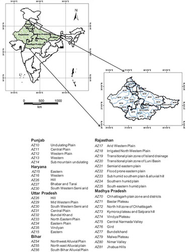
The study area is spread over 40 agroclimatic subzones (Ghosh 1991) distributed over six states of India: Punjab, Haryana, Rajasthan, Uttar Pradesh (UP), Madhya Pradesh (MP) and Bihar. Among them, two agroclimatic subzones (AZ30 & AZ15) lie both in Haryana and UP. These subzones represent diverse cropping patterns put to irrigated and rainfed conditions. The agricultural area for both kharif and rabi seasons varies from 4.2 to 25.5 m ha (million hectare) with different cropping intensities having the lowest and the highest in Rajasthan and Punjab, respectively. Crops are grown in a wide variety of soil types consisting of new alluvial, old alluvial, desert and clay soils. The major kharif crops are maize, cotton, rice, sugarcane, pulses and millets within the study region. The dominant rabi crops are wheat, potato, mustard, gram, barley and cumin. The major kharif and rabi crops in the study region are mentioned in Table 1.

Table 1. Major rabi and kharif crops in the study region.

State	Major kharif crops	Major rabi crops
Bihar	Rice, maize, jute, sugarcane, black gram, pigeon pea, moong	Wheat, barley, lentil, peas, sunflower, linseed
Haryana	Rice, jowar, bajra, maize, sugarcane, cotton, moong	Wheat, gram, rapeseed, mustard, barley
MP	Rice, jowar, bajra, maize, jute, sugarcane, pigeon pea, moong, soyabean, groundnut	Wheat, lentil, linseed, gram, peas, rapeseed, mustard, jowar, barley
Punjab	Rice, Maize, cotton, sugarcane, pulses, jowar, bajra, peas	Wheat, gram, mustard, potato,
Rajasthan	Rice, jowar, bajra, maize, black gram, pigeon	Wheat, gram, rapeseed, mustard, cumin
UP	Rice, jowar, bajra, maize, cotton, pea, moong, soyabean, groundnut, pigeon pea,	Wheat, lentil, linseed, gram, rapeseed, mustard, barley

The study region and distribution of agroclimatic subzones over six selected states are shown in Figure 1.

Figure 1. Study area with the agroclimatic distribution of subzones with their codes. For full color versions of the figures in this paper, please see the online version.

2.2. Data used

The Indian geostationary satellite INSAT 3A was launched in 2005 with subsatellite longitude at 93.5° E. It covers one-fourth of the globe, mainly the south-east Asia, in a single snapshot. The CCD is an optical payload on board INSAT 3A satellite specifically designed to monitor vegetation and snow-cover conditions over Asia. It scans the region at one-hour interval in three spectral bands, i.e. red (0.62–0.68 μm), NIR (0.77–0.86 μm), shortwave infrared (SWIR) (1.55–1.69 μm) at spatial resolution of 1000 m and radiometric resolution of 10 bit.

INSAT 3A CCD data are available in “h5” (Hierarchal Data Format Version 5) file format with Mercator projection along with latitude and longitude files. The georegistration accuracy of INSAT 3A CCD data is one pixel over Indian landmass. The INSAT 3A CCD NDVI product is generated by an operational processing after vicarious calibration (Singh, Bhattacharya, and Kulkarni 2013) of band radiances with IRS P6 AWiFS, cloud masking and atmospheric correction with standard global atmospheric products using Simple Model for Atmospheric Correction (SMAC) (Nigam et al. 2011). The CCD NDVI data were validated with the MODIS Terra global NDVI products over known land targets. The root mean square error (RMSE) between the two was 0.14 with correlation coefficient (r) 0.84 (Nigam et al. 2011). The NDVI products (product code: 3A-CCD-NDV) at 0700 GMT (Greenwich Mean Time) between 1 September 2009 and 31 March 2010 were used as training data-sets to standardize shape parameters of NDVI temporal profile over different subzones. Further, NDVI data in 2010–2011 and 2011–2012 were used for estimation of progress of crop area with the zone-specific model parameters. NDVI data for 2013–2014 was specifically used to estimate rabi crop area for comparison with high resolution derived crop area at ground observation points.

The land-use and land-cover (LULC) map prepared from SPOT-VGT at spatial resolution of 1000 m over India (Agarwal et al. 2003) was used to segregate permanent agricultural area from the nonagricultural area (e.g. waterbody, barren land, cities and forest).

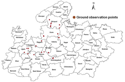
The AWiFS on board ResourceSat-2 (RS-2) satellite observes Earth’s surface in four optical bands (green (0.52–0.59 μm), red (0.62–0.68 µm), NIR (0.77–0.86 μm) and SWIR (1.55–1.70 μm)) having spatial resolution of 56 m. AWiFS has a radiometric resolution of 12 bits and swath of 740 km with 5-day repetitivity (Nigam et al. 2014). Multidate AWiFS data of rabi season 2013–2014 for October–March period for parts of MP were used to estimate rabi area at 22 ground observation points at 2 km × 2 km grid.

The ground survey was carried out over MP in 10 districts, respectively, during 3–8 March 2014 at 22 locations as shown in Figure 2.

Figure 2. Ground observation points over MP for rabi area estimation.

3. Methodology

3.1. Analysis for bidirectional reflectance distribution function

The reflecting properties in relation to surface geometry are defined by bidirectional reflectance distribution function (BRDF) f_r, (Nicodemus et al. 1977) in the following way:

(1)

where sr⁻¹ = per steradian; dL_r = reflected radiance; dE_i = incident irradiance; θ = zenith angle; φ = azimuthal angle; i = incident directions; r = viewing directions; and E_i = incident irradiance.

The absolute method to determine f_r of a sample requires measurements of both dL_r and dE_i using a spectroradiometer (using same detector). The satellite-derived surface reflectances are generally directional and depend upon the incident solar and viewing angles, though scattering due to atmosphere tries to smooth out this effect. To study the BRDF effect of INSAT 3A CCD NDVI, approximately 10,000 radiative transfer simulations using 6S (second simulation of a satellite signal in the solar spectrum) (Vermote et al. 1997) were performed. The simulations were performed for various combinations of the solar zenith angles (0, 10, 20, 30, 40, 50, 60 degrees), view zenith angles (0, 25, 30, 35, 40, 45 degrees) and relative azimuth angles (125 and 150 degrees) for a fixed atmosphere (aerosol optical depth = 0.2, aerosol model = continental, water vapor = 1.0 g cm⁻² and ozone = 0.3 cm atmosphere) for the radiances of irrigated wheat (~84% cover in six selected states). The red and NIR band radiances were atmospherically corrected for Lambertian assumption and for BRDF using Roujean model (Roujean, Leroy, and Deschamps 1992). This model takes surface objects as vertical opaque protrusions that reflect as Lambertian and cast shadows. This model can well represent the canopies with low transmittance, and takes care of the reciprocity (interchange of satellite/sensor zenith angles). It can be specified using three parameters (weights). The first one specifies the Lambertian reflectance and the other two specify the hot spot features (especially off-nadir viewing in dense canopies).

3.2. Generation of NDVI training database

The quality of daily NDVI is often degraded by the presence of cloud and fog (Forster 1984) as well as by sensor-related artifacts (Richards 1986). Among several methods, MVC of NDVI minimizes cloud contamination, atmospheric attenuation and impact of surface directional reflectance due to view and illumination geometry (Holben 1986). The MVC selects the highest observation for each pixel from a predefined compositing period. The MVC is simple and widely applied globally to monitor vegetation dynamics (Kasischke et al. 1993; Potter and Brooks 1998). In the present study, the constant viewing geometry of the geostationary satellite helps eliminate the problem of data selection far away from the subsatellite point generally encountered with polar orbiting satellites. Here, the daily NDVI data at 0700 GMT were used to generate the 10-day NDVI composites. The most stable NDVI from INSAT 3A CCD reaches between 0500 GMT and 0900 GMT in a day (Nigam et al. 2012) over the Indian subcontinent (68°–97°E, 8°–37°N).

The INSAT 3A CCD NDVI and permanent agriculture map from SPOT-VGT were coregistered at same projection (geographical latitude longitude) and datum (WGS 84) for the study area. Each agroclimatic subzone was divided into four quadrants and five sets of NDVI temporal profiles were sampled from each quadrant. These five sampling points were chosen leaving margin from the borders of quadrant to avoid “border effect” as shown in Figure 3. Similar sampling approach was followed by Bhattacharya et al. (2011), Chaurasia et al. (2011) and Vyas et al. (2013) in different studies related to agriculture and satellite remote sensing. A set of 20 such NDVI profiles within an agroclimatic subzone corresponding to four quadrants were extracted. Then, the average profile for respective agroclimatic subzone was generated from 20 such NDVI profiles. This average NDVI temporal profile was used for model training using the 10-day NDVI MVC between 1 September 2009 and 31 March 2010.

Figure 3. (a) Four quadrants of an agroclimatic zone. (b) Sampling points of NDVI profile within one quadrant of an agroclimatic zone.

3.3. Shape modeling of NDVI temporal profile

A mathematical function has been fitted to model the characteristic shape of mean NDVI profile in each agroclimatic subzone using the training data-sets during 2009–2010. The growth and decay of vegetation is not symmetric hence quadratic model was inappropriate. A cubic model was found to be the best fit to define the shape of NDVI profile in each agroclimatic subzone as shown in Figure 4.

Figure 4. Characteristic NDVI profile, dotted line shows actual profile and continuous line shows fitted profile.

The generalized form of the model is represented by the following equation:

(2)

where, “a”, “b”, “c” and “d” are the coefficients of cubic model and y is NDVI at xth dekad.

The first derivative of Equation (2) was obtained in the quadratic form Equation (3). The minima (NDVI_min) and maxima (NDVI_max) were derived from Equation (3). These two act as thresholds of NDVI temporal profile.

(3)

Further, rate of change (dy/dx) of NDVI per dekad within the limits of minima and maxima was computed from Equation (3). All these model parameters have been standardized for each subzone using the training databases. The R² and F-test were carried out for each subzone. The cubic models for each subzone showed R² between 0.78 and 0.92 and its “p” value always less than 0.00001. This is quite satisfactory performance of the each model over respective subzones. These were subsequently used in 2010–2011, 2011–2012 and 2013–2014 to estimate rabi crop area. The detailed flow of methodology is shown in Figure 5.

Figure 5. Overview of methodology for determining in-season progress of rabi cropped area using daily INSAT 3A CCD NDVI data.

3.4. Determination of predictive power of NDVI function

Sometimes noise in the NDVI leads to false rise or fall rather than actual increase or decrease in NDVI over time. The noise includes those originated from curve fit, BRDF effect, atmospheric correction scheme, cloud screening and sensor calibration. The noise in terms of number of days was calculated. Equation (2) may be written as

(4)

Equation (2) represents the signal in the form of fNDVI(t) and ∆ is the random noise with zero mean. The total variance of NDVI around time “t” describes the total information (signal and noise) contained in NDVI(t). Assuming that NDVI and ∆ are independent to each other, the total variance, Var(NDVI) is expressed as

(5)

Now, Var(fNDVI(t)) may be written as

(6)

[dfNDVI(t)/dt]² is the NDVI variance per unit time and is treated as a measure of the information in the NDVI signal observed at time “t”. The Var(t) is the variance around time (t). The Var(∆) represents variance of residual between the predicted NDVI from Equation (4) and observed NDVI. Var(∆) is equal to the square of root mean square error (RMSE²). The RMSE in the numerator represents the noise in NDVI function. Hmimina et al. (2013) defined the predictive power of the NDVI function at time (t) as

(7)

Here D(t) is the number of days (time unit) required for NDVI(t) to exceed the noise. Hence, D(t) was computed as uncertainty of NDVI model function on a given date (t). It represents the noise-to-signal ratio translated into number of days required for registering an actual rise in NDVI over and above the false rise due to noise.

3.5. Rabi crop mask generation from AWIFS

Multidate AWiFS data for different dates from October 2013 to March 2014 were used to classify rabi crops. The spectral–temporal profiles for different rabi crops were generated using stack of NDVI images of crop growing season. Multidate NDVI images of October–March period and ground observations of rabi crops were used to generate spectral–temporal profiles of rabi crops like wheat, pulses, mustard, potato, etc., at 2 km × 2 km grid at ground observation points. Nonagriculture areas were delineated through clustering by their typical NDVI values throughout the season.

4. Results and discussion

4.1. Effect of BRDF on INSAT 3A CCD NDVI

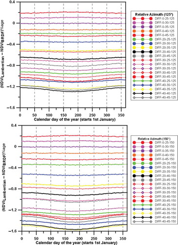
The percentage of NDVI difference between Lambertian assumption and BRDF compensation at two different azimuth angles 125° and 150° in a year at 5-day interval is shown in Figure 6. The NDVI differences were approximately 1.5% for the solar zenith angles varying from 0° to 40° and view zenith angles varying from 0° to 45° which are within the extreme imaging conditions of INSAT 3A CCD. This has an absolute impact of +0.002 to −0.017 on the NDVI. This difference is insignificant and may introduce an error of not more than 1.5% in the absolute NDVI within a year. Previously, Lee and Kaufman (1986) studied the effects of surface anisotropy on the VI and showed that the Lambertian assumption can be used safely, except the backscattering region (where solar zenith angle = view zenith angle and relative azimuth angle = 0). Recently, Franch et al. (2013) also found the differences of NDVI (Lambertian assumption with BRDF compensation) within 1%. In the present study, two consecutive 10-day NDVI composites decide the slope of the model. It is observed from the present analysis that maximum absolute change in NDVI due to BRDF within 20 days could be around 0.001 for same acquisition time (0700 GMT). Thus, 10-day NDVI composites had negligible impact due to BRDF, thereby propagating least noise.

Figure 6. Percent NDVI difference for Lambertian assumption with BRDF compensation for two different azimuth angles (DIFF-θ_s-θ_v-φ_sv).

4.2. Quantification of predictive power of NDVI shape function

The first derivative of fitted model was used as change in NDVI slope between two dekads for estimation of rabi crop area. The RMSE of first derivative was used to quantify the probable signal noise value. This (refer Section 3.4) corresponds to the number of days required to register an NDVI temporal change higher than noise. The uncertainty (noise), expressed in number of days along with standard deviation for each subzone, was computed and summarized in Table 2 for all the six states.

Table 2. Maximum and standard deviation of uncertainties in number of days calculated for six states derived from the fitted NDVI curve over agroclimatic zones.

State	Maximum	Standard deviation
Bihar	8	2
Haryana	3	0.5
MP	7.5	3
Punjab	4	1
Rajasthan	6	1.5
UP	6	1

The states of Haryana and Punjab showed minimum number of days (3–4 days) to obtain actual change in NDVI above noise. Whereas for UP, MP and Rajasthan, it ranges from 6 to 8 days with maximum 8 days occurred in Bihar. The temporal change in 10-day NDVI composite was able to overcome the uncertainties of 3–8 days due to noise. This demonstrated that the fitted mathematical functions on 10-day NDVI were robust and were able to overcome the noise for tracking increase in crop area with the passage of time during rabi season.

4.3. Characteristic NDVI temporal profiles for model training

The characteristic temporal profile of NDVI can be divided into two phases: Phase 1 (declining phase) and Phase 2 (incremental phase). Phase 1 continues from a peak around 2nd dekad to a low around 8th to 10th dekad after 1st September. Phase 2 starts increasing afterwards and reaches peak around 18th to 20th dekad. The change from Phase 1 to Phase 2 represents the transition period from kharif to rabi growing seasons. The profile characteristics largely differ across different agroclimatic subzones due to differences in cropping pattern, soil and climate. The standardized profile parameters (NDVI_min, NDVI_max) derived from NDVI cubic model and rate of change of NDVI per dekad, extracted over all the 40 agroclimatic subzones from training databases, are summarized in Table 3.

Table 3. Ranges of model parameters for characteristic NDVI temporal profiles over training sites.

State	Minimum NDVI threshold(NDVImin)	Maximum NDVI threshold(NDVImax)	Rate of change per dekad
Bihar	0.21–0.23	0.65–0.68	0.01–0.02
Haryana	0.21–0.24	0.65–0.69	0.01–0.04
MP	0.22–0.25	0.68–0.70	0.01–0.07
Punjab	0.22–0.25	0.68–0.70	0.01–0.06
Rajasthan	0.25–0.33	0.61–0.69	0.01–0.02
UP	0.23–0.25	0.50–0.58	0.01–0.03

The NDVI_min in the agroclimatic subzones in the six states varied from 0.21 to 0.33 throughout the rabi season. In homogenous agricultural area such as Punjab and Haryana, NDVI_min varied from 0.22 to 0.25. In heterogeneous agricultural area such as MP and Rajasthan, it was 0.21 to 0.33. The sign of spectral emergence of rabi crops was detected in almost all the agroclimatic subzones by the end of 2nd dekad of December (December 11–20). The increment in the rabi progress area in a particular agroclimatic subzone reaches its peak about 3–4 dekads after first detection due to saturation in the rate of change of NDVI. The characteristic NDVI profiles in each agroclimatic subzone within each state are shown in Figure 7.

Figure 7. Temporal NDVI profiles over training sites of agroclimatic zones within study area.

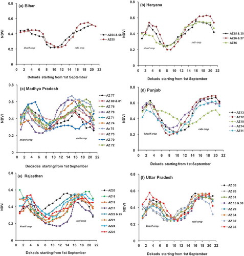
Each subzone showed different temporal NDVI profiles mainly due to differences in timing of maturity of preceding crop and emergence of next crop. In Bihar, the kharif crops include rice, maize and pulses followed by wheat and oilseed in rabi season having different lengths of growing period. This can be clearly observed from unique NDVI profiles of subzones. The major crops in Haryana are rice, cotton and pearl millet in kharif season. Among them, cotton matures during 2nd to 3rd dekad of November while rice and pearl millet mature in October and September, respectively. The crops such as wheat and mustard are dominant rabi crops in all the three subzones of Haryana. The cotton-dominant subzone (AZ16) showed delayed rise in NDVI profile as compared to other NDVI profiles in rabi season due to late harvest of cotton crop. MP is divided into 11 agroclimatic subzones. The crops such as rice, sorghum, maize and pulses are grown in kharif season followed by wheat, gram and oilseed in rabi season. All subzones showed unique NDVI profiles with different maturity and sowing time of kharif and rabi crops, respectively. Punjab typically follows rice–wheat cropping pattern with lump patches of cotton and pulses in kharif season, and potato and sugarcane in rabi season. The late maturity of cotton in kharif and late sowing of potato in rabi season in some subzones (AZ13 and AZ10) showed late rise of NDVI profile in rabi season. The pearl millet, sorghum and maize are the major crops in Rajasthan in kharif. The wheat, mustard and gram are major crops in rabi season. Among all the agroclimatic subzones in Rajasthan, the subzone, AZ19, is dominated by early sown mustard crop showing early rise of NDVI profile while late maturity of cotton crop showed late rise in the subzone, AZ17. The state of Uttar Pradesh has diverse cropping patterns in kharif and rabi seasons. The major crops in kharif are rice, maize, pulses and barley followed by wheat, oilseed, potato and sugarcane in rabi season. All the subzones showed different NDVI profiles in terms of peak and slope during rabi season.

4.4. Validation of model estimates of crop area

The crop area estimates at the end of rabi season for each state in 2010–2011 and 2011–2012 were compared with the reported rabi area issued by Department of Agriculture and Cooperation (DAC), Ministry of Agriculture, Government of India (Table 4).

Table 4. Comparison of final estimates of rabi cropped area (m ha) with reported rabi cropped area.

	2010–2011			2011–2012
State	Reported area	Estimated area	Difference in area (%)	Reported area	Estimated area	Difference in area (%)
Bihar	3.4	3.9	12.8	3.5	4.1	14.6
Haryana	3.2	3.6	11.1	3.3	3.8	13.2
MP	9.57	8.1	−18.1	10.0	8.6	−16.3
Punjab	3.6	4.1	12.2	3.5	4.0	12.5
Rajasthan	5.8	6.6	12.1	6.1	6.8	10.3
UP	12.8	13.6	5.9	12.7	13.4	5.2

Note: Here, % difference in area = ((X₁ − X₂)/X₁) × 100; X₁ = estimated area (m ha); and X₂ = reported area (m ha).

The area estimates were close to the reported area with slight overestimation in Punjab, Haryana, UP, Rajasthan and Bihar in both the years and underestimation in MP only. Though, the area was underestimated in MP for both the years, but the developed model with standardized parameter for INSAT 3A NDVI was able to capture the increasing trend of rabi area from 2010–2011 to 2011–2012 in all the six states as shown in Table 4. The overall RMSE of the estimated area for 2 years was observed 0.81 (m ha) with mean absolute error of 0.72 (m ha) and 12.5% deviation from the mean.

A marginal increase of rabi crop area was observed in all the states after second dekad of February due to identification of late sown crops and heterogeneous patches in both the years. Dekadal increase in the rabi area is shown in Figure 8.

Figure 8. Progress of rabi cropped area estimated in million hectares.

During 2010–2011, the percent deviation of estimates was minimum in UP (5.9%) and maximum in MP (−18.1%) as compared to reported data. In 2011–2012, minimum and maximum deviations were observed in UP (5.2%) and in MP (−16.3%), respectively. The percentages of deviations in 2 years between estimated (INSAT) and the reported (DAC) area could be due to the contamination of NDVI by thin persistent fog over the north and north-west India during the rabi season. MP showed the highest underestimation in both the seasons. In MP, the diversity of rabi crops was large due to mixed cultivation of cereals, pulses, oilseeds and millets. Moreover, these crops were sown under irrigated, rainfed or residual soil moisture conditions. The agriculture was also widely distributed over plain to plateau regions. All these factors might lead to large subpixel heterogeneity in NDVI growth behavior in MP. Rest of the states showed overestimation. The other five states were having more homogenous grids as compared to MP. Moreover, the INSAT CCD pixels having less than 100% crop fraction were also marked as rabi area. It overestimates the final rabi area due to mixed pixel errors in coarse resolution. The presence of mixed pixels located at the boundary between agricultural and nonagricultural classes also overestimates the total area (De Wit and Clevers 2004). In Rajasthan, the availability of irrigation water was a major constraint for sowing of rabi crops. As soon as water is available at the start of growing season, sowing is done in a synchronized manner over a large area leading to homogeneity. This resulted into the least deviation (6.8% in both the seasons) in the crop area estimates.

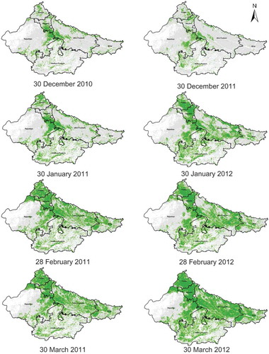
The incremental spatial distribution of the rabi crop area for 2010–2011 and 2011–2012 are shown in Figure 9. The dekadal increment in the rabi area showed that 90% of the total rabi area could be detected by 2nd dekad (20th) of February in both the years.

Figure 9. Spatial distribution for progress of rabi cropped area.

The percent change in area during 2011–2012 over 2010–2011 follows similar trends both in the estimates as well as in the reported area in all the six states as shown in Figure 10. The correlation coefficient of 0.89 (offset = 1.4 and slope = 0.48) was found between these two. This showed that the developed mathematical model with INSAT 3A CCD 1000 m NDVI was able to capture the year-to-year fluctuations in rabi area in each state.

Figure 10. Percent difference of rabi cropped area estimates and reported area in 2011–2012 from 2010–2011.

Notes: %difference in reported area = ((Reported area (2011–2012) − Reported area (2010–2011))/(Reported area (2011–2012))) × 100. %difference in INSAT 3A CCD-estimated area = ((Estimated area (2011–2012) − Estimated area (2010–2011))/(Estimated area (2011–2012)))  × 100.

4.5. Subpixel heterogeneity and crop area tracking

To evaluate the accuracy of estimated rabi area progression under homogeneous and heterogeneous regions, a 5000 m × 5000 m grid was overlaid over permanent agricultural area under study. A cluster of 25 pixels of 1000 m × 1000 m size were covered within 5000 m × 5000 m grid. The grid having a cluster of 20 or more pixels of agricultural area was categorized as homogeneous whereas grid having 12–19 pixels as semihomogeneous. The grid having a cluster of less than 12 pixels of agricultural area was categorized as heterogeneous grid as shown in Figure 11.

Figure 11. Spatial distribution of homogeneous, semihomogeneous and heterogeneous grids over the study area.

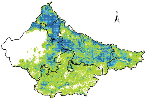
It has been observed that states such as Rajasthan and MP having more heterogeneous grids showed late estimation of rabi crop area. This could be due to subpixel heterogeneity within the footprint of grid and might cause delay in the estimation of rabi area due to low NDVI in the respective zones. The homogeneous patches in agroclimatic subzones in Punjab, Haryana and UP were identified rabi area early in the season as NDVI profile satisfied the mathematical model by attaining the thresholds for NDVI and subsequent positive rate of change of NDVI.

The agroclimatic subzones having maximum number of homogeneous and semihomogeneous grids showed early detection of rabi area as compared to subzones having more heterogeneous grids. Haryana (48%) and Punjab (42%) showed maximum percentage of homogeneous grids followed by UP (23%), Bihar (12%), Rajasthan (7%) and MP (3%), respectively. The percentages of heterogeneous grids were maximum in MP (60%) and Bihar (44%) followed by UP (28%), Rajasthan (22%), Punjab (16%) and Haryana (13%) . In contrast, some subzones of MP and Rajasthan showed early detection of rabi area in heterogeneous grid due to early sowing of rabi crops as compared to other grids. The early sown rabi crops showed early vegetative stage in the season and hence increase in the NDVI in such grids.

4.6. Comparison of INSAT 3A CCD and high resolution AWiFS-estimated rabi crop area

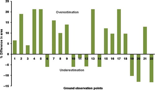
The rabi crop area from INSAT 3A CCD was estimated at 22 ground observations points over 10 districts of MP at 2 km × 2 km grid for 2013–2014. The rabi area estimated from CCD was compared with estimates of high-resolution AWiFS data up to 28 February 2014 at 2 km × 2 km grid over ground observation points. Overall 14 grids showed overestimation as compared to estimates of AWiFS and it ranged between 4% and 22%. But eight grids showed underestimation between 2% and 13% as shown in Figure 12. For 22 ground observation points, INSAT 3A CCD-estimated rabi crop area showed RMSE of 0.52 km² and 16.36% deviation from mean of AWiFS-estimated area at 2 km × 2 km grid.

Figure 12. Percent difference in final estimates of rabi cropped area between INSAT 3A CCD and AWIFS at 2 km × 2 km grid over ground observation points.

5. Conclusions

This study demonstrated the potential of the high temporal multispectral observations from Indian geostationary satellite (INSAT 3A) to monitor in-season continuous temporal progress of rabi crop area. The characteristic cubic pattern of NDVI profile across the transition of two consecutive crop growing seasons could differentiate growth patterns among agroclimatic subzones due to differences in crop types and sowing patterns. The change in 10-day NDVI composite was able to overcome the noise generated from the model for all agroclimatic subzones. The standardized model parameters were able to capture the year-to-year fluctuation in rabi crop area in line with the reported area. The validation of area estimates showed mean deviation ranging from 14.6% to −18.1% with respect to reported DAC statistics during rabi seasons of 2010–2011 and 2011–2012. INSAT- estimated rabi crop area showed 16.36% deviation from AWiFS derived rabi area at 2 km × 2 km grid.

Subpixel heterogeneity due to coarser spatial resolution of CCD and diversity of crop types over fragmented land holdings in India is a major concern in such satellite-based crop area estimates. In heterogeneous grids, NDVI was affected by mixed signals from crop and noncrop patches in the subpixel which produced lump response. This further delayed the estimation of rabi crop area in heterogeneous grids as compared to homogeneous grids. This suggests that sensor with finer spatial resolution (~50 m) and spectral resolution at par with IRS P6 AWiFS having temporal resolution of CCD will be able to produce better and frequent crop area estimates. This would be possible through ISRO’s (Indian Space Research Organization’s) proposed future mission of GISAT (Geostationary Imaging Satellite) which will provide multispectral observations at 56 m from geostationary satellite platform.

The policy-makers and user agencies require dynamic and regular monitoring of progress in rabi crop area from early part of the season till its termination. The present study demonstrated that data from geostationary satellites sensors could be used to systematically and objectively monitor rabi crop area at an interval of 10 days with reliable accuracy. The proposed methodology is now being implemented by user agency (Mahalanobis National Crop Forecast Centre, New Delhi) on experimental basis to track rabi crop area on near real time.

Disclosure statement

No potential conflict of interest was reported by the authors.

Acknowledgments

Authors are grateful to Shri A.S. Kiran Kumar, Chairman ISRO, for his motivation, encouragement and keen interest in this study. The author would also like to thank Shri Tapan Misra, Director Space Applications Centre, ISRO, for his support. The authors wish to acknowledge Meteorological Oceanographic Satellite Data Archival Centre (MOSDAC), SAC, for providing in-season INSAT 3A CCD NDVI data. The authors would like to express their sincere appreciation to anonymous reviewers for their valuable comments to improve this article.

References

- Agarwal, S., P. K. Joshi, Y. Shukla, and P. S. Roy. 2003. “Spot Vegetation Multi-Temporal Data for Classifying Vegetation in South Central Asia.” Current Science 84: 1440–1448.
- Bacour, C., F.-M. Bréon, and F. Maignan. 2006. “Normalization of the Directional Effects in NOAA–AVHRR Reflectance Measurements for an Improved Monitoring of Vegetation Cycles.” Remote Sensing of Environment 102: 402–413. doi:10.1016/j.rse.2006.03.006.
- Badhwar, G. D. 1984. “Use of Landsat-Derived Profile Features for Spring Small-Grains Classification.” International Journal of Remote Sensing 5: 783–797. doi:10.1080/01431168408948860.
- Bauer, M. E. 1985. “Spectral Inputs to Crop Identification and Condition Assessment.” Proceedings of the IEEE73: 1071−1085.
- Bhattacharya, B. K., K. Mallick, R. Nigam, K. Dakore, and A. M. Shekh. 2011. “Efficiency Based Wheat Yield Prediction in a Semi-Arid Climate Using Surface Energy Budgeting with Satellite Observations.” Agricultural and Forest Meteorology 151: 1394–1408. doi:10.1016/j.agrformet.2011.06.002.
- Chang, J. C., M. C. Hansen, K. Pittman, M. Carroll, and C. DiMiceli. 2007. “Corn and Soybean Mapping in the United States Using MODIS Time-Series Data Sets.” Agronomy Journal 99: 1654–1664. doi:10.2134/agronj2007.0170.
- Chaurasia, S., R. Nigam, B. K. Bhattacharya, V. N. Sridhar, K. Mallick, S. P. Vyas, N. K. Patel, et al. 2011. “Development of Regional Wheat VI-LAI Models Using ResourceSat-1 AWiFS Data.” Journal of Earth System Science 120: 1113–1125. doi:10.1007/s12040-011-0126-x.
- Congalton, R. G., M. Balogh, C. Bell, K. Green, J. A. Milliken, and R. Ottman. 1998. “Mapping and Monitoring Agricultural Crops and Other Land Cover in the Lower Colorado River Basin.” Photogrammetric Engineering and Remote Sensing 64: 1107−1113.
- De Beurs, K. M., and G. M. Henebry. 2010. “A Land Surface Phenology Assessment of the Northern Polar Regions Using MODIS Reflectance Time Series.” Canadian Journal of Remote Sensing 36: S87–S110. doi:10.5589/m10-021.
- De Wit, A. J. W., and J. G. P. W. Clevers. 2004. “Efficiency and Accuracy of Per-Field Classification for Operational Crop Mapping.” International Journal of Remote Sensing 25: 4091−4112. doi:10.1080/01431160310001619580.
- Delbart, N., T. L. Toan, L. Kergoat, and V. Fedotova. 2006. “Remote Sensing of Spring Phenology in Boreal Regions: A Free of Snow-Effect Method Using NOAA-AVHRR and SPOT-VGT Data (1982–2004).” Remote Sensing of Environment 101: 52–62. doi:10.1016/j.rse.2005.11.012.
- Department of Agriculture & Cooperation. 2012. “State of Indian Agriculture 2011–12.” http://agricoop.nic.in/sia111219912.pdf
- Duchemin, B., J. Goubier, and G. Courrier. 1999. “Monitoring Phenological Key Stages and Cycle Duration of Temperate Deciduous Forest Ecosystems with NOAA/AVHRR Data.” Remote Sensing of Environment 67: 68–82. doi:10.1016/S0034-4257(98)00067-4.
- Fensholt, R., and S. R. Proud. 2012. “Evaluation of Earth Observation Based Global Long-Term Vegetation Trends – Comparing GIMMS and MODIS Global NDVI Time Series.” Remote Sensing of Environment 119: 131–147. doi:10.1016/j.rse.2011.12.015.
- Fensholt, R., K. Rasmussen, T. T. Nielsen, and C. Mbow. 2009. “Evaluation of Earth Observation Based Long-Term Vegetation Trends – Intercomparing NDVI Time Series Trend Analysis Consistency of Sahel from AVHRR GIMMS, Terra MODIS and SPOT VGT Data.” Remote Sensing of Environment 113: 1886–1898. doi:10.1016/j.rse.2009.04.004.
- Fensholt, R., I. Sandholt, S. Stisen, and C. Tucker. 2006. “Analysing NDVI for the African Continent Using the Geostationary Meteosat Second Generation Seviri Sensor.” Remote Sensing of Environment 101: 212–229. doi:10.1016/j.rse.2005.11.013.
- Forster, B. C. 1984. “Derivation of Atmospheric Correction Procedures for Landsat MSS with Particular Reference to Urban Data.” International Journal of Remote Sensing 5: 799–817. doi:10.1080/01431168408948861.
- Franch, B., E. F. Vermote, J. A. Sobrino, and E. Fédèle. 2013. “Analysis of Directional Effects on Atmospheric Correction.” Remote Sensing of Environment 128: 276–288. doi:10.1016/j.rse.2012.10.018.
- Ghosh, S. P., ed. 1991. Agro-Climatic Zone Specific Research, Indian Perspective under N.A.R.P. New Delhi: Indian Council of Agricultural Research.
- Hmimina, G., E. Dufrêne, J.-Y. Pontailler, N. Delpierre, M. Aubinet, B. Caquet, A. De. Grandcourt, et al. 2013. “Evaluation of the Potential of MODIS Satellite Data to Predict Vegetation Phenology in Different Biomes: An Investigation Using Ground-Based NDVI Measurements.” Remote Sensing of Environment 132: 145–158. doi:10.1016/j.rse.2013.01.010.
- Holben, B. N. 1986. “Characteristics of Maximum-Value Composite Images from Temporal AVHRR Data.” International Journal of Remote Sensing 7: 1417–1434. doi:10.1080/01431168608948945.
- Höpfner, C., and D. Scherer. 2011. “Analysis of Vegetation and Land Cover Dynamics in North-Western Morocco during the Last Decade Using MODIS NDVI Time Series Data.” Biogeosciences 8: 3359–3373. doi:10.5194/bg-8-3359-2011.
- Huete, A., K. Didan, T. Miura, E. P. Rodriguez, X. Gao, and L. G. Ferreira. 2002. “Overview of the Radiometric and Biophysical Performance of the MODIS Vegetation Indices.” Remote Sensing of Environment 83: 195–213. doi:10.1016/S0034-4257(02)00096-2.
- Kang, S. Y., S. W. Running, J. H. Lim, M. S. Zhao, C. R. Park, and R. Loehman. 2003. “A Regional Phenology Model for Detecting Onset of Greenness in Temperate Mixed Forests, Korea: An Application of MODIS Leaf Area Index.” Remote Sensing of Environment 86: 232−242. doi:10.1016/S0034-4257(03)00103-2.
- Kasischke, E. S., N. H. F. French, P. Harrell, N. L. Christensen, S. L. Ustin, and D. Barry. 1993. “Monitoring of Wildfires in Boreal Forests Using Large Area AVHRR NDVI Composite Image Data.” Remote Sensing of Environment 45: 61–71. doi:10.1016/0034-4257(93)90082-9.
- Lee, T. Y., and Y. J. Kaufman. 1986. “Non-Lambertian Effects on Remote Sensing of Surface Reflectance and Vegetation Index.” IEEE Transactions on Geoscience and Remote Sensing GE-24: 699–708. doi:10.1109/TGRS.1986.289617.
- Meng, Q., W. H. Cooke, and J. Rodgers. 2013. “Derivation of 16-Day Time-Series NDVI Data for Environmental Studies Using a Data Assimilation Approach.” GIScience & Remote Sensing 50: 500–514.
- Nicodemus, F. E., J. C. Richmond, J. J. Hsia, I. W. Ginsberg, and T. Limperis. 1977. “Geometrical Considerations and Nomenclature for Reflectance.” NBS Monogr., No. 160, U.S. Department of Commerce, National Bureau of Standards, 52.
- Nigam, R., B. K. Bhattacharya, K. R. Gunjal, N. Padmanabhan, and N. K. Patel. 2012. “Formulation of Time Series Vegetation Index from Indian Geostationary Satellite and Comparison with Global Products.” Journal of the Indian Society of Remote Sensing 40: 1–9. doi:10.1007/s12524-011-0122-2.
- Nigam, R., B. K. Bhattacharya, R. K. Gunjal, N. Padmanabhan, and N. K. Patel. 2011. “A Continental Scale Vegetation Index from Indian Geostationary Satellite.” Current Science 10: 1184–1192.
- Nigam, R., B. K. Bhattacharya, S. Vyas, and M. P. Oza. 2014. “Retrieval of Wheat Leaf Area Index from AWiFS Multispectral Data Using Canopy Radiative Transfer Simulation.” International Journal of Applied Earth Observation and Geoinformation 32: 173–185. doi:10.1016/j.jag.2014.04.003.
- Oza, M. P., M. R. Pandya, and D. R. Rajak. 2008. “Evaluation and Use of ResourceSat-I Data for Agricultural Applications.” International Journal of Applied Earth Observation and Geoinformation 10: 194–205. doi:10.1016/j.jag.2008.02.006.
- Oza, M. P., D. R. Rajak, N. Bhagia, S. Dutta, S. P. Vyas, N. K. Patel, and J. S. Parihar. 2006. “Multiple Production Forecasts of Wheat in India Using Remote Sensing and Weather Data.” Proceedings of SPIE 6411: 102–108.
- Pan, Y., L. Li, J. Zhang, S. Liang, X. Zhu, and D. Sulla-Menashe. 2012. “Winter Wheat Area Estimation from MODIS-EVI Time Series Data Using the Crop Proportion Phenology Index.” Remote Sensing of Environment 119: 232–242. doi:10.1016/j.rse.2011.10.011.
- Parihar, J. S., and M. P. Oza. 2006. “FASAL: An Integrated Approach for Crop Assessment and Production Forecasting.” Proceeding of SPIE 6411: 1–13.
- Potter, C. 2014. “Regional Analysis of MODIS Satellite Greenness Trends for Ecosystems of Interior Alaska.” GIScience & Remote Sensing 51: 390–402. doi:10.1080/15481603.2014.933606.
- Potter, C. S., and V. Brooks. 1998. “Global Analysis of Empirical Relations between Annual Climate and Seasonality of NDVI.” International Journal of Remote Sensing 19: 2921–2948. doi:10.1080/014311698214352.
- Rajak, D. R., M. P. Oza, N. Bhagia, and V. K. Dadhwal. 2005. “Spectral Wheat Growth Profile in Punjab Using IRS WiFS Data.” Journal of the Indian Society of Remote Sensing 33: 345–352. doi:10.1007/BF02990055.
- Reed, B. C., J. F. Brown, D. VanderZee, T. R. Loveland, J. W. Merchant, and D. O. Ohlen. 1994. “Measuring Phenological Variability from Satellite Imagery.” Journal of Vegetation Science 5: 703–714. doi:10.2307/3235884.
- Reed, B. C., T. R. Loveland, and L. L. Tieszen. 1996. “An Approach for Using AVHRR Data to Monitor US Great Plains Grasslands.” Geocarto International 11: 13−22. doi:10.1080/10106049609354544.
- Richards, J. A. 1986. Remote Sensing and Digital Image Analysis, 281. New York: Springer-Verlag.
- Roujean, J.-L., M. Leroy, and P.-Y. Deschamps. 1992. “A Bidirectional Reflectance Model of the Earth’s Surface for the Correction of Remote Sensing Data.” Journal of Geophysical Research 97: 20455–20468. doi:10.1029/92JD01411.
- Rouse, J. W., R. H. Has, J. A. Schell, D. W. Deering, and J. C. Harlan. 1974. Monitoring the Vernal Advancement of Retrodgradation of Natural Vegetation. NASA/GSFC, Type III, Final Report, 371. Greenbelt, MD: Texas A & M University.
- Sakamoto, T., A. A. Gitelson, and T. J. Arkebauer. 2013. “Modis-Based Corn Grain Yield Estimation Model Incorporating Crop Phenology Information.” Remote Sensing of Environment 131: 215–231. doi:10.1016/j.rse.2012.12.017.
- Sakamoto, T., M. Yokozawa, H. Toritani, M. Shibayama, N. Ishitsuka, and H. Ohno. 2005. “A Crop Phenology Detection Method Using Time-Series MODIS Data.” Remote Sensing of Environment 96: 366–374. doi:10.1016/j.rse.2005.03.008.
- Singh, S. K., B. K. Bhattacharya, and A. Kulkarni. 2013. “ Cross Calibration of INSAT 3A CCD Channel Radiances with IRS P6 AWiFS Sensor.” Journal of Earth System Science 122: 957–966. doi:10.1007/s12040-013-0318-7.
- South, S., J. Qi, and D. P. Lusch. 2004. “Optimal Classification Methods for Mapping Agricultural Tillage Practices.” Remote Sensing of Environment 91: 90−97. doi:10.1016/j.rse.2004.03.001.
- Telesca, L., and R. Lasaponara. 2006. “Quantifying Intra-Annual Persistent Behaviour in SPOT-VEGETATION NDVI Data for Mediterranean Ecosystems of Southern Italy.” Remote Sensing of Environment 101: 95–103. doi:10.1016/j.rse.2005.12.007.
- Tucker, C. J. 1979. “Red and Photographic Infrared Linear Combinations for Monitoring Vegetation.” Remote Sensing of Environment 8: 127–150. doi:10.1016/0034-4257(79)90013-0.
- Verbeiren, S., H. Eerens, I. Piccard, I. Bauwens, and J. V. Orshoven. 2008. “Sub-Pixel Classification of SPOT-VEGETATION Time Series for the Assessment of Regional Crop Areas in Belgium.” International Journal of Applied Earth Observation and Geoinformation 10: 486–497. doi:10.1016/j.jag.2006.12.003.
- Vermote, E. F., D. Tanre, J. L. Deuze, M. Herman, and J.-J. Morcette. 1997. “Second Simulation of the Satellite Signal in the Solar Spectrum, 6S: An Overview.” IEEE Transactions on Geoscience and Remote Sensing 35: 675–686. doi:10.1109/36.581987.
- Vyas, S., R. Nigam, N. K. Patel, and S. Panigrahy. 2013. “Extracting Regional Pattern of Wheat Sowing Dates Using Multispectral and High Temporal Observations from Indian Geostationary Satellite.” Journal of the Indian Society of Remote Sensing 41: 855–864. doi:10.1007/s12524-013-0266-3.
- White, M. A., K. De Beurs, K. Didan, D. W. Inouye, A. D. Richardson, O. P. Jensen, J. O’keefe, et al. 2009. “Intercomparison, Interpretation, and Assessment of Spring Phenology in North America Estimated from Remote Sensing for 1982–2006.” Global Change Biology 15: 2335–2359. doi:10.1111/j.1365-2486.2009.01910.x.
- Xiao, X., S. Boles, S. Frolking, W. Salas, B. Moore, C. Li, L. He, and R. Zhao. 2002. “Observation of Flooding and Rice Transplanting of Paddy Rice Fields at the Site to Landscape Scales in China Using VEGETATION Sensor Data.” International Journal of Remote Sensing 23: 3009−3022. doi:10.1080/01431160110107734.
- Yuan, F., C. Wang, and M. Mitchell. 2014. “Spatial Patterns of Land Surface Phenology Relative to Monthly Climate Variations: US Great Plains.” GIScience & Remote Sensing 51: 30–50. doi:10.1080/15481603.2014.883210.
- Zhang, X., M. A. Friedl, C. B. Schaaf, A. H. Strahlera, J. F. C. Hodges, F. Gao, B. C. Reed, and A. Huete. 2003. “Monitoring Vegetation Phenology Using MODIS.” Remote Sensing of Environment 84: 471–475. doi:10.1016/S0034-4257(02)00135-9.
- Zhong, L., P. Gong, and G. S. Biging. 2012. “Phenology-based Crop Classification Algorithm and its Implications on Agricultural Water Use Assessments in California’s Central Valley.” Photogrammetric Engineering & Remote Sensing 78: 799–813. doi:10.14358/PERS.78.8.799.