Modeling aboveground biomass of an alpine desert grassland with SPOT-VGT NDVI

Abstract

Grassland biomass on the Qinghai-Tibet Plateau is of great significance for the study of wildlife habitat and climate change. Based on Systéme Pour l’Observation de la Terre Vegetation normalized difference vegetation index (NDVI) data from 1998 to 2012 and a field survey investigation in 2013, we assessed aboveground biomass (AGB) dynamics in the Altun Mountain Nature Reserve. The results demonstrated that annual NDVI values varied greatly with an increasing trend. Areas of high- and medium-coverage grassland showed similar increasing trends. The NDVI–biomass relationship could be quantified by an exponential model and previous models overestimated the amount of biomass in the alpine desert grassland. The total biomass was estimated to be 62 × 10⁶ kg per year with large annual variations. No significant relationship was found between AGB and soil organic carbon contents, and the total grassland area (NDVI > 0.1) was positively correlated with the annual average temperature.

Keywords:

• climate change
• vegetation change
• soil organic carbon
• NDVI
• Altun Mountain Nature Reserve

1 Introduction

The terrestrial biosphere is now strongly affected by climate change, especially with regard to vegetation (De Jong et al. 2011). Grassland covers approximately one-third of the total area of China forming the dominant land cover in the Qinghai-Tibet Plateau (Ma et al. 2010). Using an environmental vulnerability index (EVI), Wang et al. (2008) have demonstrated that more than 50% of the Tibetan Plateau is ecologically vulnerable (e.g., EVI > 2.7). Alpine grassland, which is a fragile ecosystem, may be most affected by global warming. Characterizing the relationship between grassland ecosystem dynamics and climate change is crucial for grassland management and biodiversity conservation (Parton et al. 1995). The quantification of such relationship will also facilitate the provision of many ecosystem services, including biodiversity preservation, production of livestock forage, and carbon (C) storage. Among all these ecosystem services, the amount of aboveground biomass (AGB) is the most important factor that will determine forage availability and herbivore carrying capacity (Yahdjian and Sala 2006). Knowledge of grassland soil organic carbon (SOC) dynamics is also critical to clarify the contribution of grassland ecosystems to the global C budget. Studies have shown that terrestrial ecosystems on the Qinghai-Tibet Plateau act as a small carbon sink (Piao et al. 2009). However, approximately 10% of the SOC stock in the grasslands could be lost in response to an increase of temperature by 2°C (Tan et al. 2010).

Biomass harvesting is a basic method that is used for estimating AGB for terrestrial ecosystems. However, it is difficult to quantify ecosystem dynamics on temporal and spatial scales due to the lack of applicable field data (Ouyang et al. 2012; Propastin 2013). On a macroscopic scale, traditional field data sets could be complemented by continuous information provided from remote sensing (RS) (Kross et al. 2011). RS data at relatively high spatiotemporal resolution have been widely used to estimate grassland biomass at regional, continental, and global scales (e.g., Seaquist, Olsson, and Ardö 2003; Piao et al. 2005; Chen et al. 2007; Yang et al. 2009; Li et al. 2013). Geographic information systems (GIS) and RS can be used to derive additional information (Wang et al. 2008) and can serve as powerful tools for ecological assessments such as regional ecological risk (Xu et al. 2004), environmental degradation (Bastin, Pickup, and Pearce 1995; Holm, Cridland, and Roderick 2003), ecological restoration (Li and Potter 2012), landscape pattern (Propastin 2013), and landscape change (Gustafson et al. 2005). Many studies have investigated the relationship between AGB and precipitation, temperature, soil texture, and biophysical parameters in grassland or forest ecosystems (Epstein, Lauenroth, and Burke 1997; Huang, He, and Niu 2013; Da Silva et al. 2014; Gleason and Im 2011). Other studies have focused more on carbon storage capacity, photochemical rate, and forage production using high-resolution lidar data, hyperspectral reflectance data or medium resolution Fraction of Vegetation Cover (fCover) product time series (Reader and Miller 2014; Lee, Kim, and Choi 2013; Roumiguié et al. 2015). At large scales, the normalized difference vegetation index (NDVI) (derived from satellite data) and the Carnegie–Ames–Stanford Approach model have been successfully used to estimate vegetation production and biomass (Wessels et al. 2004; Piao et al. 2005; Wang, Li, and Wang 2007). Dryland ecosystems account for approximately 47% of the Earth’s total land surface area (Lal 2001), and recent studies have shown that dryland is very important in terrestrial C dynamics, as these areas may act as carbon sinks (Wohlfahrt, Fenstermaker, and Arnone 2008). In alpine grasslands, especially in alpine deserts, a comprehensive assessment of biomass dynamics and C stock is still not available.

Discussion and controversy have arisen concerning different methods to estimate AGB (Piao et al. 2007), especially in grassland ecosystems. Many studies have utilized AGB estimation models based on RS data and spatial analysis (Xin et al. 2009; Du, Liu, and Guo 2011). Relationships between soil, climate, topography, and other influential factors on AGB distribution have been extensively studied (e.g., Sala et al. 1988; Epstein, Lauenroth, and Burke 1997), especially in temperate regions. On the Tibetan Plateau, various quantitative relational models between NDVI and biomass have been developed (Zhang et al. 2010; Feng et al. 2011). Most of these models have been applied to alpine meadows and for estimating the seasonal biomass production of grassland dairy systems. Biomass estimation for alpine deserts, however, has not been well explored (Piao et al. 2007). Additionally, few studies have incorporated biomass data and SOC data that were measured in the field (Yang et al. 2009).

The Qinghai-Tibet Plateau is the largest and highest plateau on Earth. The Altun Mountain National Nature Reserve (AMNRR) is located at the northern border of the Plateau with a mean elevation of 4500 m. This region, known as one of the four largest so-called “no-man’s lands” in China, is a “geographical blank region,” and its ecological status and change have not been addressed due to its inaccessibility, high elevation, enormous area, severe weather, and limited land vehicular access during rainy seasons. The natural vegetation in this reserve is dominated by alpine grasslands with limited anthropogenic disturbance. Thus, the reserve is ideal for investigating AGB dynamics. Previous research has indicated that NDVI could be a good indicator of gazelle habitat, although the NDVI alone cannot explain the seasonal migration of gazelles (Ito et al. 2006). It is important to evaluate the effectiveness of NDVI as an indicator of habitat quality. These studies of biomass change are vital for wildlife protection, habitat protection, and nature reserve management.

Grassland degradation is one of the most widespread and severe environmental issues on the Qinghai-Tibet Plateau (Wang, Li, and Wang 2007), especially in the arid and semiarid areas in which vegetation is susceptible to climatic variations. Climate change causes desertification, oasis degradation, and increase in drought frequency (Ling, Xu, and Zhang 2011). In arid and semiarid ecosystems, vegetation production is strongly correlated with seasonal values of multitemporal NDVI (Ma et al. 2010; Cong et al. 2012). The AMNNR is located in Xinjiang Uygur Autonomous Region, where the grasslands mainly consist of species that have adapted to alpine desert conditions. Studies have shown, over the past 50 years, that significant climate changes have taken place here (Zhang, Wang, and Wang 2012; Tang and Xu 2010); however, a better understanding of NDVI and biomass must be gained to accurately document the effects of climate change on the grassland ecosystems in the AMNNR. Furthermore, the uniqueness of its climate, vegetation, and nonanthropogenic activities makes this an ideal region for monitoring AGB in desert grasslands.

This study is to investigate the spatial distribution and dynamics of biomass in grassland ecosystems in the AMNNR using a combination of ground survey and RS data. In particular, we will (1) establish an NDVI–biomass model for alpine desert grassland in this region, (2) compare the model results with other NDVI–biomass models, and (3) explore the relationship between biomass and influencing environmental factors.

2 Methods

2.1 Study area

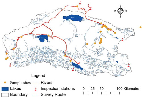
The AMNNR, which was established in May 1983, is located in the northwestern part of the Qinghai-Tibet Plateau. The AMNNR was designed to protect alpine ecosystems and is currently a habitat for many endangered animals, including the Tibetan antelope (Pantholops hodgsonii), Tibetan wild donkey (Asinus kiang), and wild yak (Bos grunniens). There are more than 63 animal species of higher taxonomic order and 300 plant species of higher taxonomic order. They lie in Qarkilik (Ruoqiang) County, Kuerle prefecture, Xinjiang Uygur Autonomous Region, adjacent to Lop Nur in the north and Kekexili and the Qiangtang National Nature Reserve in the east and south, respectively. The reserve lies between 87°10ʹ E to 91°18ʹ E and 36°00ʹ N to 37°49ʹ N and has a total area of more than 45,000 km² (Figure 1). The AMNNR is bordered by the Kunlun Mountains to the south and the Altun Mountains to the north. The elevation ranges from 3700 to 6900 m. The annual precipitation is approximately 250 mm, and the mean air temperature is below 0°C. There are large daily fluctuations in temperature, and precipitation varies spatially due to various topographical conditions.

Figure 1. Location of the study area. For full colour versions of the figures in this paper, please see the online version.

Corresponding to differences in climatic conditions and topography, vegetation types in the AMNNR show an ecophysiographic gradient from alpine desert steppe, alpine and mountainous talus sparse grassland, alpine steppe, alpine cushion grassland, alpine shrub, to swamp meadow. The alpine steppe is the main vegetation type, and the dominant graminoids are Stipa, Kobresia, and Carex spp. The spatial extent of the reserve and associated biomass are important factors that impact the abundance of endangered wildlife.

2.2 Data collection and processing

Systéme Pour l’Observation de la Terre Vegetation (SPOT-VGT) time-series 10-day composite images (www.vgt.vito.be) derived from the vegetation instrument of the SPOT 4 and 5 satellites were acquired to analyze NDVI change. These data were processed with a maximum value compositing (MVC) method to reduce errors resulting from cloud cover and large solar zenith angles (Holben 1986). The MVC method retains only the highest spectral value on a per-pixel basis for a series of multitemporal, georeferenced satellite sensor data. The spatial resolution of SPOT NDVI is 1/112°, or approximately 1 km, and the temporal resolution is approximately 10 days, which makes 36 composites per year (Cong et al. 2012; Maisongrande, Duchemin, and Dedieu 2004). We focused on the period from April 1998 to November 2012, with a total of 527 composites. Additionally, NDVI data in July 2013 were used for AGB modeling. Each composite consists of a digital number (DN) file and a status map (SM) file, which describe potential problems that were observed for the reflectance of each band (Tchuenté et al. 2011). During the data analysis process, inland water areas and man-made areas were masked. NDVI values were calculated using DN values as follows:

(1)

DN values were originally saved as eight bytes per pixel with values from 0 to 255. Using this formula, that is, scale = 0.004 and offset = −0.1, the real dimension of the NDVI index values were derived, which were restricted to the range between −0.096 (DN = 1) and 0.92 (DN = 255) compared with the range [−0.1, 0.92] of the original NDVI that were provided by the SPOT/VEGETATION. The slight loss at the bottom of the NDVI range does not affect the data quality because it never concerns clear land observations (mostly water). The yearly NDVI (NDVI_year) was calculated by averaging the monthly maximum NDVI based on a per pixel basis, which provided annual information about the grassland conditions in the study region. The formula was calculated as follows:

(2)

where NDVI_month is the monthly maximum NDVI. NDVI_month was calculated by maximizing the three 10-day sets of data including NDVI1, NDVI2, and NDVI3, which refer to the maximum NDVI in the first 10 days, second 10 days, and third 10 days of each month, respectively.

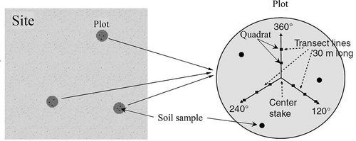
Grassland biomass was measured in July 2013 at 24 sites that were located within the grassland area of the AMNNR (Figure 1). NDVI values are highest during July of each year. Because summer is a rainy season in the AMNNR, access by vehicle is restricted in proximity to wetlands and open bodies of water. At each site, we ensured that the topography was flat and that the grassland homogeneously covered at least 1000 × 1000 m² area within the corresponding pixel of the SPOT-NDVI product. Based on the method of Hankins, Launchbaugh, and Hyde (2004), three 30 m line-transects as one plot within each site were established, originating from the same base point at the center of the 100 m × 100 m plot and each transect separated by a 120°angle. On each line-transect, three 1 m × 1 m small quadrats located at 10, 20, and 30 m distances were set for biomass harvesting. Three duplicated plots were established within a single site (Figure 2) (Tang et al. 2015). A total of 27 biomass samples were collected at each site (Hankins, Launchbaugh, and Hyde 2004). AGB was clipped and the live plant material and dead plant material were separated. The weight of the live plant material was recorded for each site and the samples were weighed again after being dried for 48 h at 70°C in the lab. This study further categorized the grassland into three types based on the NDVI levels: low-coverage grassland (0.1 < NDVI < 0.15), middle-coverage grassland (0.15 < NDVI < 0.2), and high-coverage grassland (NDVI > 0.2) according to the field survey.

Figure 2. Schematic of the sampling method for the vegetation survey in the study region.

To estimate the SOC content and relate it to the AGB, we conducted in situ soil sampling and laboratory analysis. Soil samples were collected from the 0–20 cm soil layer at three random locations using a soil drill on each plot. The soil samples were air dried and sieved through a 2-mm mesh for soil carbon analysis. The widely used dichromate oxidation method based upon the Walkely–Black procedure was used to measure the SOC (%), as it is simple, rapid, and has minimal equipment needs (Nelson and Sommer 1975).

To determine the influence of climate change on AGB, precipitation and temperature data from 1998 to 2012 were analyzed to determine the relationship between NDVI and precipitation and temperature. Precipitation and temperature data were derived from 16 National Meteorological Stations located close to the study area. Liu et al. (2014) indicated that regional average values of monthly precipitation and temperature are able to indicate the climate condition of the study area (Liu et al. 2014). Then, average annual values of precipitation and temperature were calculated to indicate the climate change from 1998 to 2012 (Partal and Kahya 2006).

2.3 Grassland biomass modeling

This study aims to determine a reasonable value for the quantity of AGB in desert grassland. First, we evaluated the feasibility of eight previously established NDVI–biomass models based mainly on grassland by reviewing the related published literature (Table 1). Further, we modeled the relationship between the NDVI and AGB by using field data acquired from AMNNR.

Table 1. Comparison of different NDVI–biomass models.

No.	NDVI (x)–biomass (Y) equation	Model types	Study region	NDVI data source	Reference
1	Y = 29.44e^1.49x	Exponential model	Alpine grassland	GIMMS	Xin et al. 2009
2	Y = 268.810e^2.398x	Exponential model	Qinghai-Tibet Plateau	MODIS	Feng et al. 2011
3-1 3-2	Y = 0.0108x^2 + 4.1536x – 78.012	Quadratic polynomial model	Qinghai-Tibet Plateau	MODIS	Du, Liu, and Guo 2011
	Y = 11.187*e^0.0485x	Exponential model	Qinghai-Tibet Plateau	MODIS
4	Y = 109.29e^3.85x	Exponential model	Qinghai-Tibet Plateau	MODIS	Chu et al. 2007
5	Y = 13389x^2.4587	Power function	Qinghai-Tibet Plateau	MODIS	Fang et al. 2011
6	Y = 26.38e^3.8725x	Exponential model	Northern China	GIMMS	Ma et al. 2010
7	Y = 179.71x^1.6228	Power function	China	GIMMS	Piao et al. 2007
8	Y = 375.16 + 1.029x1 + 0.204x2 + 9.047x3 – 0.0340x4 – 0.0736x5	Regression model	Alpine grassland	SPOT-VGT	Zhang et al. 2010

Note: GIMMS, Global Inventory Modelling and Mapping Studies; MODIS, Moderate Resolution Imaging Spectroradiometer.

2.4 Statistical analyses

The spatiotemporal variability of AGB can be affected by many factors. The relationship between annual AGB amount (kg) and temperature and precipitation was analyzed using regression analysis. Additionally, using the field AGB data for spatial variability, the relationship between the site-specific AGB and the corresponding SOC data was investigated. The coefficient of determination (R²) was used to evaluate the performance of the regression equations. All of the statistical analyses were conducted using the SPSS 17.0 software package (SPSS, Chicago, IL, USA).

3 Results

3.1 Temporal dynamics and spatial distribution of NDVI

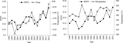
The seasonal fluctuation of NDVI values corresponds to the status of vegetation within a year. However, we found the peak NDVI value that occurred early in August (the Julian day is approximately 240) had an approximately 1-month lag in terms of the highest temperature and precipitation, both of which reached their maxima in July. Similarly, between January and February the minimum NDVI values occurred when temperature and precipitation were lowest (Figure 3). The temperature showed a similar trend with NDVI variation, although the peak points and lowest points were not completely identical for the same year. The relationship between precipitation and NDVI, although apparent, is not very strong. Careful observation indicates that there were three precipitation peak periods: 2002, 2005, and after 2008 (Figure 3). Corresponding to these precipitation peaks, NDVI increased from 2002 to 2007 and again after 2008. These results implied that the wet years have impacted NDVI or the grassland status, although the impact may have a time lag.

Figure 3. Dynamics of NDVI, temperature, and precipitation from 1998 to 2012.

The NDVI value is relatively low at the regional scale due to large proportions of the study area being desert, rock, or glaciers. On a monthly timescale, most of the NDVI values were less than 0.1. Temperature and precipitation have the ability to create fluctuations of the NDVI values, thus, the correlations between the temperature, precipitation, and NDVI were analyzed at monthly and annual time intervals (Table 2). At a monthly interval, both the temperature and precipitation were highly correlated with NDVI, whereas the exponential regression models had higher correlations (R²) than the linear regression models. At an annual time intervals, only the temperature showed a significant relationship with the NDVI values, whereas the precipitation had no significant relationship. The regression model adequately described the relationship between NDVI, temperature, and precipitation in the grassland coverage.

Table 2. Temporal regression equations for grassland NDVI at monthly and annual time scales.

Scale	Variables	Regression models for NDVI (Y)
		Exponential	R^2	Linear	R^2
Monthly	Temperature (x)	Y = 0.0484e^0.0258x	0.717**	Y = 0.0016x + 0.0492	0.659**
	Precipitation (x)	Y = 0.0444e^0.0071x	0.742**	Y = 0.0005x + 0.0435	0.708**
Annual	Temperature (x)	Y = 0.1474e^0.0898x	0.523**	Y = 0.0118x + 0.1469	0.548**
	Precipitation (x)	Y = 0.1229e^0.0001x	0.001 ns	Y = 2E-05x + 0.1226	0.002 ns

Notes: **Significant at <0.01 level; ns, no significance.

As the low NDVI values were apt to be affected by the underlying earth surface with a low grassland coverage, we only considered the average values of the NDVI pixels that were greater than or equal to 0.1 (Fang et al. 2004). Referring to the vegetation map of the nature reserve, grasslands mainly exist in the areas where the NDVI value is > 0.1.

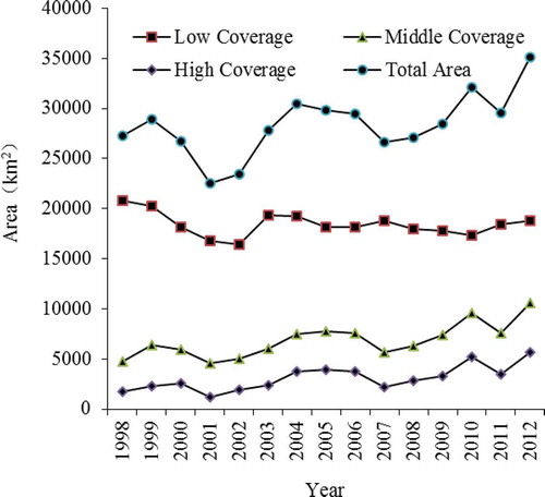
The NDVI value has a strong relationship with the grassland growing conditions and AGB. It is obvious that large-scale spatial variability exists in the region. In the center of the AMNNR, the NDVI values were relatively higher. Relatively lower NDVI values were observed in the northern and southern parts of the study region. The lower value areas were dominated by bare lands, saline and alkaline lands, deserts, or glaciers. These areas are mainly located in the Ayaku Lake basin. According to our field investigation, there are needle grasslands (Stipa spp.) distributed in the central part near the Kaerdun inspection station (dark green). This area is also a main habitat for the wild ungulates. Using GIS reclassification, the areas of the three grassland types were calculated. Figure 4 shows the grassland time series in 1998, 2003, 2007, and 2012. A comparison of these four maps reveals that the spatial distribution of the grasslands varies greatly. The area of grassland was severely reduced during the drought year of 2007. Changes in the different coverage areas from 1998 to 2012 are presented in Figure 5. The results indicate that the low-coverage grassland comprises the largest proportion of land area in the study site, whereas the high-coverage grassland comprises the lowest proportion. With respect to a real extent on an annual basis, the middle-coverage and high-coverage grasslands were variable with similar oscillation trends. The annual trend for the low-coverage grassland was slightly different than for the middle-coverage and high-coverage grasslands. Specifically, the high- and middle-coverage grasslands had an increasing trend with fluctuations, whereas the low-coverage grassland had a decreasing trend. The total area had an overall upwards trend, which indicated a mild increase in grasslands with relatively significant fluctuations over the past 15 years. In 2001 and 2002, the grassland area decreased significantly. In 2007 and 2008, the grassland area was also slightly smaller.

Figure 4. Time series NDVI distribution in typical years (1998, 2003, 2007, and 2012).

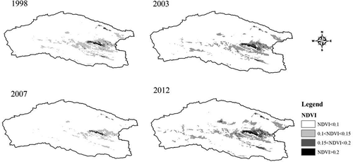
Figure 5. Trends of the grassland coverage at different levels from 1998 to 2012.

3.2 Estimation of aboveground biomass

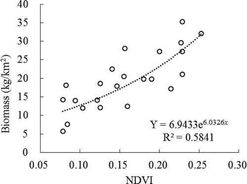
The living grass biomass in the small subplots at each site was averaged and the values were correlated with the NDVI data. The results show that the maximum NDVI is approximately 0.4, which is relatively low for grassland. The field data revealed that the AGB values ranged from 5 to 40 kg/km², which corresponded to the coverage ranging from 5% to 30% according to the field survey. As shown in Figure 6, the fitted exponential equation regression model had an acceptable coefficient of determination. The simulated model is expressed as follows: Y = 6.9433e^6.0326x (R² = 0.58, n = 24). The NDVI values were treated as the predictor variable and the biomass served as the dependent variable (Table 3).

Figure 6. Relationship between AGB and growing season NDVI in 2013.

3.3 Comparison of different models

Field information for the alpine desert grassland in the AMNNR is still limited, especially in the “no-man’s” land. Although we investigated AGB in 2013, the resources that were available to the investigators were not sufficient, which restricted the field measurements to only a fraction of the community types in the region. In that case, we assessed the suitability of the models that were derived from the literature review for comparison as listed in Table 1. These regression-based models were derived from different areas of China but most of them were based in the Qinghai-Tibet grassland. We assumed there were no significant differences between the NDVI values, although the data were derived from different sensor systems. The suitability of the models for the alpine desert grassland is assessed in Table 3. We calculated the ranges for the simulated NDVI values that fell between 0.1 and 0.4 using these models. Most of the models that are listed were based on ground data from alpine meadows and alpine steppes. Some of the models were not feasible based on the simulated values. Our results show that AGB simulated by models 2, 3-1, 4, and 5 were much larger than the field survey value of 70 kg/km², whereas model 7 simulated AGB was lower than the field measurement. In addition, models 1, 3-2, 6, and 8 simulated AGB were close to field measurements for the alpine desert grassland. Therefore, our comparison was focused on the simulated AGB results using those four models (e.g., 1, 3-2, 6, and 8).

Table 3. Description of different models and suitability assessment for alpine desert grassland.

No.	Calculated AGB value (kg/km^2) (0.1 < x < 0.4)	Value rationality for measured value range (<80 kg/km^2)	Model comparison	Suitability
1	34.17–53.43	Within the range	Based on alpine grassland in China	Yes
2	341.66–701.49	Too large	Based on alpine meadow data from the Qinghai-Tibet Plateau	No
3-1	−35.4–105.41	Negative values when NDVI < 0.2	Based on grassland data from the Qinghai-Tibet Plateau	No
3-2	18.17–77.85	Within the range	Another equation in the same article above	Yes
4	160.61–509.79	Too large	Based on alpine meadow data from the Qinghai-Tibet Plateau	No
5	46.56–1407.13	Too large	Data from the Qinghai-Tibet Plateau	No
6	38.86–124.16	Within the range	Data stems from northern China	Yes
7	4.28–40.63	Too low	Based on grassland from all China	No
8	51.49–86.89	Within the range	Based on alpine grassland	Yes

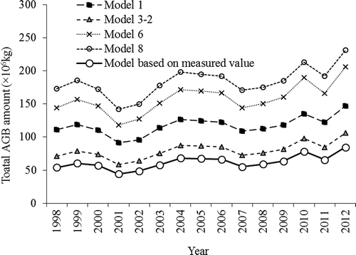
The simulated AGB results using models 1, 3-2, 6, and 8 are presented in Figure 7. Considerable differences can be found between the curves that were based on the linear models and those that were based on the exponential models, especially when the NDVI value was larger than 0.5. A more detailed comparison for NDVI less than 0.4 is shown in Figure 8. The simulated AGB values ranged from 20 to 120 kg/km². The simulated model for the field investigation, expressed by Y = 6.9433e^6.0326x (Figure 6), is also presented in Figure 8. Most of the actual field measurements were clearly lower than the results of the models. Using the ArcGIS spatial analysis, we calculated the total amount of AGB in the nature reserve over the past 15 years. The results indicated that the annual absolute AGB values varied greatly between different models, whereas the yearly trends for the period from 1998 to 2012 were very similar. Generally, model 8 had the largest value (183.5 × 10⁶ kg) followed by model 6 (157.8 × 10⁶ kg), model 1 (117.4 × 10⁶ kg), and model 3-2 (79.9 × 10⁶ kg). The model developed using field surveys gave a smaller AGB value than the four models that were described above, with a total AGB of 62.04 × 10⁶ kg for the entire AMNNR. The dynamics of AGB based on the different methods are shown in Figure 9.

Figure 7. Model-simulated AGB for different NDVI–biomass models.

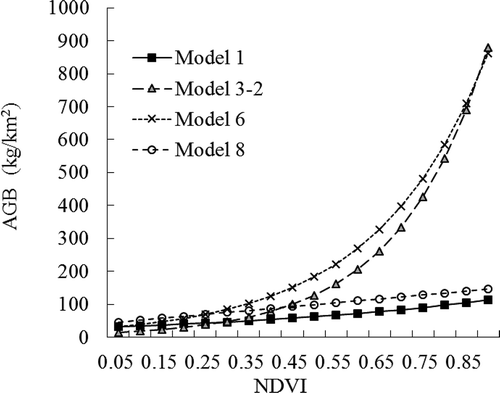
Figure 8. Comparison between the referred NDVI–biomass models and the simulated models based on the measured biomass values.

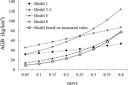
Figure 9. Total biomass change in the past 15 years in the AMNNR.

3.4 Relationship between AGB and influencing environmental variables

In the study region, AGB may be affected by soil, climate, and topographical and other environmental covariates. Temporally, annual AGB dynamics are closely related with the annual or monthly variations in temperature and precipitation, whereas at the local scale, site-specific soil fertility is an important environmental factor. The relationships between AGB and SOC for all of the sites are shown in Figure 10a, and no significant correlation was found. Presumably, this lack of correlation is related to the large variation in the SOC content when the biomass was low, for example, and ranged from 10 to 25 kg/km².

Figure 10. Relationship between AGB and SOC: (a) all sites; (b) Stipa grasslands.

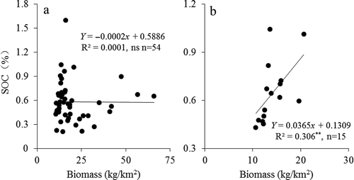
SOC contents ranged from 0.19% to 1.8%, with nearly an order of magnitude difference between the different grassland types. In addition, SOC contents had a significant relationship with biomass for the Stipa grassland (Figure 10b). When plotted against all types of grassland in the study area, the relationship between SOC and AGB did not show a strong and consistent pattern, presumably due to elevation difference, topographic variability, and soil heterogeneity.

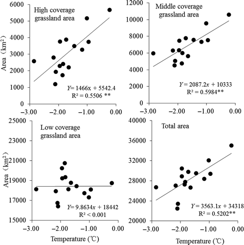
The results also show a positive, strong linear correlation between the total AGB amount and the annual temperature (R² = 0.543, P < 0.01) in the AMNNR for the period 1998–2012 (Figure 11). This relationship was even stronger for high-coverage grassland (R² = 0.55, P < 0.01) and medium-coverage grassland (R² = 0.60, P < 0.01). Whereas an insignificant relationship between AGB and the annual temperature was found for the low-coverage grassland (R² = 0.520, P < 0.01) (Figure 12). The linear regression did not reveal a significant relationship between the precipitation and AGB.

Figure 11. Relationship between total AGB in AMNNR and annual average temperature.

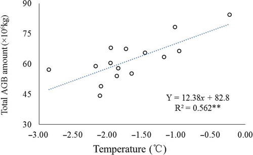
Figure 12. Relationship between grassland area and temperature.

4 Discussion

4.1 The effectiveness of the NDVI method and the simulated model

Satellite-based indicators are advantageous for monitoring the spatial and temporal variations of changes in vegetation at regional scales due to their large-area and frequent coverage (Su et al. 2003). Recently, numerous studies have examined the relationship between NDVI and biomass based on field investigations in China, especially for the Qinghai-Tibet Plateau. Some studies indicated that NDVI can approach saturation in cases of moderate to high density of vegetation (Gitelson 2004). Whereas in the area of low-coverage alpine desert grassland, NDVI may serve as a reliable indicator for AGB, as it is strongly correlated with regional terrestrial ecological status (Ouyang et al. 2012). The relationship between NDVI and AGB is usually described by regression-based models (Table 1). Results of the study revealed that not all of the models could be used to accurately reflect vegetation growth conditions for this specific climate zone nor this “no man’s” land at the border of the Qinghai-Tibet Plateau.

Yang et al. (2009) pointed out that in the AMNNR region the capacity to protect wildlife and fragile ecosystems and to predict the consequences of global change are partially dependent upon our understanding of spatiotemporal patterns and their environmental controls on AGB. In alpine grasslands of China, information on the spatial and temporal distribution of AGB and its governing environmental variables is far less extensive than for temperate grassland (Piao et al. 2007). For alpine desert grassland, even less data are available. Using the published NDVI–biomass model for grassland in China, we assessed the relative variability of AGB in the AMNNR and used four different estimation equations with different parameters. The results indicated that equations that were derived at a large scale in the Qinghai-Tibet Plateau may overestimate the amount of AGB in the AMNNR. Although greater differences in AGB estimation existed among these models, the trends are similar for NDVI values ranging from 0.1 to 0.4.

It is noteworthy that these NDVI–biomass models use different data sources. NDVI is not a biophysical parameter; rather, it is a quantity derived from reflectance measurements in the red and the NIR bands. Thus, it is dependent on the band specifications of the sensors. For the models compared in this study, data sources were from a MODIS data set (models 2, 3, 4, and 5), GIMMS data (models 1, 6, and 7), and SPOT-VGT (model 8). Some studies have compared the efficiency and difference using GIMMS, MODIS, and SPOT-VGT series in China (Du et al. 2014; Song et al. 2010; Liu and Zhou 2015). Their results showed that there is significant linear relationship between MODIS and SPOT-VGT NDVI (Liu and Zhou 2015). The root-mean-square deviation for annual MODIS and SPOT-VGT NDVI is approximately 0.04 (Song et al. 2010), and GIMMS and MODIS NDVI are approximately 0.06. The differences are not particularly high for the model prediction, but it would be better if the comparison between their estimates could be made with a cross-calibration of different NDVI data in advance, that is, the joint use of data from different satellites requires inter-satellite cross-calibration. Usually, multitemporal NDVI data synthesizing procedures such as spatial aggregation, linear function between reflectance, and NDVI would be used for this purpose (Cecilia, Alfonso, and Anne 2004).

To assist the local nature reserve administration in the AMNNR, it is necessary to be aware of regional grassland conditions and the impact of climate change on this vulnerable ecosystem. Currently, a relatively accurate total carrying capacity for the three large ungulates remains unknown in the AMNNR. In addition, the migration routes of the Tibetan antelope and the distribution of the wildlife habitats remain unclear. Our study on AGB estimation is a first step toward improving rangeland management, although it is difficult for the administration of AMNNR to incorporate RS into management decisions at present.

4.2 Environmental factors influencing AGB in the AMNNR and the ecological implications

As aboveground plants are the primary source of soil C, a strong positive correlation is often found between net primary productivity and soil C content (Carrera et al. 2009). In this study, however, there was not a statistically significant relationship between AGB and SOC content. This result showed that besides the influence of AGB input on SOC, other factors such as soil taxon, topography, and soil texture could influence SOC levels. Additional research should be conducted to determine how AGB and SOC variability affects vegetation growth that is essential for large herbivore support (Muñoz García and Faz Cano 2012; Propastin 2013). Some studies have found that approximately 40–60% of soil SOC appears below a depth of 20 cm in grasslands and 2.98 ± 0.51 kg C m⁻² in high-altitude grasslands located on the Tibet Plateau at 0–10 cm (4100–5100 m.a.s.l) (Wang et al. 2008). Remotely sensed data can be used as surrogates for ecological productivity, and these data have been successfully used to predict belowground C stocks (Paruelo et al. 2010). On the Qinghai-Tibet Plateau, studies have verified that satellite RS could potentially be used for large-scale mapping of soil respiration for the carbon cycle process (Huang, He, and Niu 2013). Therefore, additional soil information is required to determine soil properties that may influence AGB.

As a “no man’s” land, long-term AGB changes in AMNNR are mainly affected by climate change. A number of studies have investigated the relationship between the spatial patterns of AGB and climate factors and soil factors in grassland ecosystems (e.g., Sala et al. 1988; Epstein, Lauenroth, and Burke 1997). The desert grassland on the Qinghai-Tibet Plateau is also expected to be sensitive to climate change. At a large scale, precipitation also strongly determines grassland AGB spatially. However, due to the lack of monitoring data of precipitation within the AMNNR and large variations and errors of predicted precipitation in the past 15 years (Liu et al. 2014), we cannot determine the relationship between AGB and precipitation.

The study indicated a significant relationship between temperature and NDVI in grasslands of AMNNR. Clearly, the average temperature in the AMNNR increased rapidly over the past 15 years. Although the complex feedbacks between temperature and precipitation may not be found in this region, the increase in temperature has likely led to an accelerated snow melt in the surrounding mountains, therefore, increased soil water content in regions with relatively low elevation.

Further research should be carried out to elucidate the ecological effects of climate change on vegetation status. In our study, only annual AGB was considered. Whereas the seasonal vegetation phenology that is affected by climate factors has an important practical significance in biodiversity conservation. Monitoring long-term trends in the biomass, plant species, and phenological characters is therefore required for nature reserve management.

5 Conclusions

Using the NDVI index, we estimated the AGB in the AMNNR for the past 15 years using existing regression-based models. The results indicated that grasslands are mainly located in the core area of the AMNNR with substantial annual variability in the coverage. The total annual AGB in the AMNNR is approximately 62 × 10⁶ kg, and the AGB in the AMNNR is significantly correlated with temperature in this region. However, the annual precipitation had no significant relationship with AGB. This study further found an exponential function between NDVI and AGB supported by the field investigations.

This study showed that AGB did not correlate with SOC at a large scale if only the grassland type was taken into account. A comparison between existing “NDVI–biomass” models and field measurements revealed that all of the calculated AGB values were overestimated, despite their trends being similar.

Future studies are needed to characterize the relationship between grassland and climate at a seasonal scale, with a particular emphasis on the influence of precipitation. With regard to the management of the nature reserve, a weather monitoring system may be established to provide necessary spatial information. Moreover, as wild antelopes are migrant animals in this nature reserve, determining grassland dynamics and patterns of the wildlife migration are also critical for conservation efforts. Furthermore, in addition to climate variables, other factors, including human activity – mainly mining in the buffer zones, soil reflectance, and grassland types – may also account for the uncertainty in the NDVI–biomass estimation. In addition, as the NDVI values in this region are very low and only values larger than 0.1 were taken into account, the total AGB may be underestimated. More detailed field information, including grassland types, soil texture, and environmental factors, is necessary to better quantify relationships between the RS indicators and vegetation in the AMNNR.

Disclosure statement

No potential conflict of interest was reported by the authors.

Additional information

Funding

The research was supported by the Nonprofit Environment Protection Specific Project of China [grant number 201209033]; National Key Technology R&D Program of China [grant number 2012BAC01B02].

References

- Bastin, G. N., G. Pickup, and G. Pearce. 1995. “Utility of AVHRR Data for Land Degradation Assessment: A Case Study.” International Journal of Remote Sensing 16: 651–672. doi:10.1080/01431169508954432.
- Carrera, A. L., M. J. Mazzarino, M. B. Bertiller, H. F. Del Valle, and E. M. Carretero. 2009. “Plant Impacts on Nitrogen and Carbon Cycling in the Monte Phytogeographical Province, Argentina.” Journal of Arid Environments 73: 192–201. doi:10.1016/j.jaridenv.2008.09.016.
- Cecilia, M. B., C. Alfonso, and J. Anne. 2004. “Intersatellite Cross-Calibration: Integration of Reflectance and NDVI from Different Satellites by Means of a Linear Model.” Remote Sensing for Agriculture, Ecosystems, and Hydrology 5232 (1): 128–139.
- Chen, Y. X., G. Lee, P. Lee, and T. Oikawa. 2007. “Model Analysis of Grazing Effect on Above-Ground Biomass and Above-Ground Net Primary Production of a Mongolian Grassland Ecosystem.” Journal of Hydrology 333: 155–164. doi:10.1016/j.jhydrol.2006.07.019.
- Chu, D., Q. M. Ji, Y. Z. Deji, and C. Pu. 2007. “Estimating Grassland Biomass in North Tibetan Plateau Using EOS/MODIS.” Acta Meteorologica Sinica 65 (4): 612–621.
- Cong, N., S. Piao, A. Chen, X. Wang, X. Lin, S. Chen, S. Han, G. Zhou, and X. Zhang. 2012. “Spring Vegetation Green-Up Date in China Inferred from SPOT NDVI Data: A Multiple Model Analysis.” Agricultural and Forest Meteorology 165: 104–113. doi:10.1016/j.agrformet.2012.06.009.
- Da Silva, R. D., L. S. Galvão, J. R. Dos Santos, C. V. De J. Silva, and Y. M. De Moura. 2014. “Spectral/Textural Attributes from ALI/EO-1 for Mapping Primary and Secondary Tropical Forests and Studying the Relationships with Biophysical Parameters.” GIScience & Remote Sensing 51: 677–694. doi:10.1080/15481603.2014.972866.
- De Jong, R., S. De Bruin, A. De Wit, M. E. Schaepman, and D. L. Dent. 2011. “Analysis of Monotonic Greening and Browning Trends from Global NDVI Time-Series.” Remote Sensing of Environment 115 (2): 692–702. doi:10.1016/j.rse.2010.10.011.
- Du, J. Q., J. M. Shu, Y. H. Wang, Y. C. Li, L. B. Zhang, and Y. Guo. 2014. “Comparison of GIMMS and MODIS Normalized Vegetation Index Composite Data for Qinghai-Tibet Plateau.” Chinese Journal of Applied Ecology 25 (2): 533–544.
- Du, Y. E., B. K. Liu, and Z. G. Guo. 2011. “Changes of Forage Biomass of Grasslands during the Growing Season in the Qinghai-Tibetan Plateau Based on MODIS Data.” Practaculture Science 28 (6): 1117–1123.
- Epstein, H. E., W. K. Lauenroth, and I. C. Burke. 1997. “Effects of Temperature and Soil Texture on ANPP in the U.S. Great Plains.” Ecology 78: 2628–2631. doi:10.1890/0012-9658(1997)078[2628:EOTAST]2.0.CO;2.
- Fang, J., X. D. Huang, W. Wang, H. Yu, L. Y. Ma, and T. G. Liang. 2011. “The Grassland Biomass Monitoring by Remote Sensing Technology in the Qinghai-Tibet Plateau.” Pratacultural Science 28 (7): 1345–1351.
- Fang, J. Y., S. L. Piao, J. S. He, and W. H. Ma. 2004. “Increasing Terrestrial Vegetation Activity in China, 1982–1999.” Science in China (C-Life Science) 47: 229–240.
- Feng, Q. S., X. H. Gao, X. D. Huang, H. Yu, and T. G. Liang. 2011. “Remote Sensing Dynamic Monitoring of Grass Growth in Qinghai-Tibet Plateau from 2001 to 2010.” Journal of Lanzhou University (Natural Sciences) 47: 75–83.
- Gitelson, A. A. 2004. “Wide Dynamic Range Vegetation Index for Remote Quantification of Biophysical Characteristics of Vegetation.” Journal of Plant Physiology 161 (2): 165–173. doi:10.1078/0176-1617-01176.
- Gleason, C. J., and J. Im. 2011. “A Review of Remote Sensing of Forest Biomass and Biofuel: Options for Small-Area Applications.” GIScience & Remote Sensing 48: 141–170. doi:10.2747/1548-1603.48.2.141.
- Gustafson, E. J., R. B. Hammer, V. C. Radeloff, and R. S. Potts. 2005. “The Relationship between Environmental Amenities and Changing Human Settlement Patterns between 1980 and 2000 in the Midwestern USA.” Landscape Ecology 20: 773–789. doi:10.1007/s10980-005-2149-7.
- Hankins, J., K. Launchbaugh, and G. Hyde. 2004. “Rangeland Inventory as a Tool for Science Education: Program Pairs Range Professionals, Teachers and Students Together to Conduct Vegetation Measurements and Teach Inquiry-Based Science.” Rangelands 26 (1): 28–32. doi:10.2111/1551-501X(2004)26[28:RIAATF]2.0.CO;2.
- Holben, B. N. 1986. “Characteristics of Maximum-Value Composite Images from Temporal AVHRR Data.” International Journal of Remote Sensing 7: 1417–1434. doi:10.1080/01431168608948945.
- Holm, A. M., S. W. Cridland, and M. L. Roderick. 2003. “The Use of Time-Integrated NOAA NDVI Data and Rainfall to Assess Landscape Degradation in the Arid Shrubland of Western Australia.” Remote Sensing of Environment 85: 145–158. doi:10.1016/S0034-4257(02)00199-2.
- Huang, N., J.-S. He, and Z. Niu. 2013. “Estimating the Spatial Pattern of Soil Respiration in Tibetan Alpine Grasslands Using Landsat TM Images and MODIS Data.” Ecological Indicators 26: 117–125. doi:10.1016/j.ecolind.2012.10.027.
- Ito, T. Y., N. Miura, B. Lhagvasuren, D. Enkhbileg, S. Takatsuki, A. Tsunekawa, and Z. Jiang. 2006. “Satellite Tracking of Mongolian Gazelles (Procapra Gutturosa) and Habitat Shifts in Their Seasonal Ranges.” Journal of Zoology 269 (3): 291–298. doi:10.1111/jzo.2006.269.issue-3.
- Kross, A., R. Fernandes, J. Seaquist, and E. Beaubien. 2011. “The Effect of the Temporal Resolution of NDVI Data on Season Onset Dates and Trends across Canadian Broadleaf Forests.” Remote Sensing of Environment 115 (6): 1564–1575. doi:10.1016/j.rse.2011.02.015.
- Lal, R. 2001. “Potential of Desertification Control to Sequester Carbon and Mitigate the Greenhouse Effect.” Climatic Change 51: 35–72. doi:10.1023/A:1017529816140.
- Lee, S. J., J. R. Kim, and Y. S. Choi. 2013. “The Extraction of Forest CO2 Storage Capacity Using High-Resolution Airborne Lidar Data.” GIScience and Remote Sensing 50: 154–171.
- Li, S., and C. Potter. 2012. “Patterns of Aboveground Biomass Regeneration in Post-Fire Coastal Scrub Communities.” GIScience & Remote Sensing 49: 182–201. doi:10.2747/1548-1603.49.2.182.
- Li, Z., T. Huffman, B. McConkey, and L. Townley-Smith. 2013. “Monitoring and Modeling Spatial and Temporal Patterns of Grassland Dynamics Using Time-Series MODIS NDVI with Climate and Stocking Data.” Remote Sensing of Environment 138: 232–244. doi:10.1016/j.rse.2013.07.020.
- Ling, H. B., H. L. Xu, and Q. Q. Zhang. 2011. “Climate Change in the Manas River Basin, Xinjiang during 1956–2007.” Journal of Glaciology and Geocryology 33 (1): 64–71.
- Liu, S. L., H. D. Zhao, S. K. Dong, N. N. An, X. K. Su, and X. Zhang. 2014. “Climate Changes in the Alpine Grassland Nature Reserves on Qinghai-Tibet Plateau in Recent 50 Years Based on SPEI Index.” Ecology and Environment Sciences 23 (12): 1883–1888.
- Liu, Y., and M. C. Zhou. 2015. “A Comparative Analysis of AVHRR, SPOT-VGT and MODIS NDVI Remote Sensing Data over Hanjiang River Basin.” Journal of South China Agricultural University 36 (1): 106–112.
- Ma, W., J. Fang, Y. Yang, and A. Mohammat. 2010. “Biomass Carbon Stocks and Their Changes in Northern China’s Grasslands during 1982–2006.” Science China Life Sciences 53 (7): 841–850. doi:10.1007/s11427-010-4020-6.
- Maisongrande, P., B. Duchemin, and G. Dedieu. 2004. “VEGETATION/SPOT: An Operational Mission for the Earth Monitoring; Presentation of New Standard Products.” International Journal of Remote Sensing 25: 9–14. doi:10.1080/0143116031000115265.
- Muñoz García, M. A., and A. Faz Cano. 2012. “Soil Organic Matter Stocks and Quality at High Altitude Grasslands of Apolobamba, Bolivia.” Catena 94: 26–35. doi:10.1016/j.catena.2011.06.007.
- Nelson, D. M., and L. E. Sommer. 1975. “A Rapid and Accurate Method for Estimating Organic Carbon in Soil.” Proceeding Indiana Academic Science 84: 456–462.
- Ouyang, W., F. H. Hao, A. K. Skidmore, T. A. Groen, A. G. Toxopeus, and T. J. Wang. 2012. “Integration of Multi-Sensor Data to Assess Grassland Dynamics in a Yellow River Sub-Watershed.” Ecological Indicators 18: 163–170. doi:10.1016/j.ecolind.2011.11.013.
- Partal, T., and E. Kahya. 2006. “Trend Analysis in Turkish Precipitation Data.” Hydrological Processes 20: 2011–2026. doi:10.1002/(ISSN)1099-1085.
- Parton, W. J., J. M. O. Scurlock, D. S. Ojima, D. S. Schimel, D. O. Hall, SCOPEGRAM Group, M. B. Coughenour, E. G. Moya, and T. G. Gilmanov. 1995. “Impact of Climate-Change on Grassland Production and Soil Carbon Worldwide.” Global Change Biology 1: 13–22. doi:10.1111/gcb.1995.1.issue-1.
- Paruelo, J. M., G. Piñeiro, G. Baldi, S. Baeza, F. Lezama, A. Altesor, and M. Oesterheld. 2010. “Carbon Stocks and Fluxes in Rangelands of the Río De La Plata Basin.” Rangeland Ecology & Management 63 (1): 94–108. doi:10.2111/08-055.1.
- Piao, S. L., J. Y. Fang, P. Ciais, P. Peylin, Y. Huang, S. Sitch, and T. Wang. 2009. “The Carbon Balance of Terrestrial Ecosystems in China.” Nature 458: 1009–1013. doi:10.1038/nature07944.
- Piao, S. L., J. Y. Fang, L. M. Zhou, K. Tan, and S. Tao. 2007. “Changes in Biomass Carbon Stocks in China’s Grasslands between 1982 and 1999.” Global Biogeochemical Cycles 21: 1–10. doi:10.1029/2005GB002634.
- Piao, S. L., J. Y. Fang, L. M. Zhou, B. Zhu, K. Tan, and S. Tao. 2005. “Changes in Vegetation Net Primary Productivity from 1982 to 1999 in China.” Global Biogeochemical Cycles 19: 1–16. doi:10.1029/2004GB002274.
- Propastin. 2013. “Large-Scale Mapping of Aboveground Biomass of Tropical Rainforest in Sulawesi, Indonesia, Using Landsat ETM+ and MODIS Data.” GIScience and Remote Sensing 50: 633–651.
- Reader, H. E., and W. L. Miller. 2014. “Application of Hyperspectral Remote Sensing Reflectance Data to Photochemical Rate Calculations in the Duplin River, a Tidal River on the Coast of Georgia, USA.” GIScience & Remote Sensing 51: 199–211. doi:10.1080/15481603.2014.895583.
- Roumiguié, A., A. Jacquin, G. Sigel, H. Poilvé, B. Lepoivre, and O. Hagolle. 2015. “Development of an Index-Based Insurance Product: Validation of a Forage Production Index Derived from Medium Spatial Resolution Fcover Time Series.” GIScience & Remote Sensing 52: 94–113. doi:10.1080/15481603.2014.993010.
- Sala, O. E., W. J. Parton, L. Joyce, and W. Lauenroth. 1988. “Primary Production of the Central Grassland Region of the United States.” Ecology 69: 40–45.
- Seaquist, J. W., L. Olsson, and J. Ardö. 2003. “A Remote Sensing-Based Primary Production Model for Grassland Biomes.” Ecological Modelling 169: 131–155. doi:10.1016/S0304-3800(03)00267-9.
- Song, F. Q., M. Y. Kang, P. Yang, Y. R. Chen, Y. Liu, and K. X. Xing. 2010. “Comparison and Validation of GIMMS, SPOT-VGT and MODIS Global NDVI Products in the Loess Plateau of Northern Shaanxi Province, Northwestern China.” Journal of Beijing Forestry University 32 (4): 72–80.
- Su, Z. B., A. Yacob, J. Wen, G. Roerink, Y. B. He, B. H. Gao, H. Boogaard, and C. Van Diepen. 2003. “Assessing Relative Soil Moisture with Remote Sensing Data: Theory, Experimental Validation, and Application to Drought Monitoring over the North China Plain.” Physics and Chemistry of the Earth, Parts A/B/C 28 (1–3): 89–101. doi:10.1016/S1474-7065(03)00010-X.
- Tan, K., P. Ciais, S. L. Piao, X. P. Wu, Y. H. Tang, N. Vuichard, S. Liang, and J. Y. Fang. 2010. “Application of the ORCHIDEE Global Vegetation Model to Evaluate Biomass and Soil Carbon Stocks of Qinghai-Tibetan Grasslands.” Global Biogeochemical Cycles 24 (1): GB1013. doi:10.1029/2009GB003530.
- Tang, D. L., and L. G. Xu. 2010. “Characteristics of Spatio-Temporal Variability of Precipitation in Xinjiang Region under the Background of Climate Change.” Journal of Water Resources and Water Engineering 21 (3): 72–76.
- Tang, L., S. K. Dong, R. Sherman, S. L. Liu, Q. R. Liu, X. X. Wang, X. K. Su, et al. 2015. “Changes in Vegetation Composition and Plant Diversity with Rangeland Degradation in the Alpine Region of Qinghai-Tibet Plateau.” The Rangeland Journal 37 (1): 107. doi:10.1071/RJ14077.
- Tchuenté, A., S. M. Jong, J. Roujean, C. Favier, and C. Mering. 2011. “Ecosystem Mapping at the African Continent Scale Using a Hybrid Clustering Approach Based on 1-Km Resolution Multi-Annual Data from SPOT/VEGETATION.” Remote Sensing of Environment 115: 452–464. doi:10.1016/j.rse.2010.09.015.
- Wang, G. X., Y. S. Li, and Y. B. Wang. 2007. “Typical Alpine Wetland System Changes on the Qinghai-Tibet Plateau in Recent 40 Years.” Acta Geographica Sinica 62 (5): 481–491.
- Wang, X. D., X. H. Zhong, S. Z. Liu, J. G. Liu, Z. Y. Wang, and M. H. Li. 2008. “Regional Assessment of Environmental Vulnerability in the Tibetan Plateau: Development and Application of a New Method.” Journal of Arid Environments 72 (10): 1929–1939. doi:10.1016/j.jaridenv.2008.06.005.
- Wessels, K. J., S. D. Prince, P. E. Frost, and D. Van Zyl. 2004. “Assessing the Effects of Human-Induced Land Degradation in the Former Homelands of Northern South Africa with a 1 Km AVHRR NDVI Time-Series.” Remote Sensing of Environment 91 (1): 47–67. doi:10.1016/j.rse.2004.02.005.
- Wohlfahrt, G., L. F. Fenstermaker, and J. A. Arnone III. 2008. “Large Annual Net Ecosystem CO2 Uptake of a Mojave Desert Ecosystem.” Global Change Biology 14: 1475–1487. doi:10.1111/j.1365-2486.2008.01593.x.
- Xin, X. P., B. H. Zhang, G. Li, H. B. Zhang, B. R. Chen, and G. X. Yang. 2009. “Variation in Spatial Pattern of Grassland Biomass in China from 1982 to 2003.” Journal of Natural Resources 24: 1582–1583.
- Xu, C., H. S. He, Y. Hu, Y. Chang, D. R. Larsen, X. Li, and R. Bu. 2004. “Assessing the Effect of Cell-Level Uncertainty on a Forest Landscape Model Simulation in Northeastern China.” Ecological Modelling 180: 57–72.
- Yahdjian, L., and O. E. Sala. 2006. “Vegetation Structure Constrains Primary Production Response to Water Availability in the Patagonian Steppe.” Ecology 87: 952–962. doi:10.1890/0012-9658(2006)87[952:VSCPPR]2.0.CO;2.
- Yang, Y. H., J. Y. Fang, Y. D. Pan, and C. J. Ji. 2009. “Aboveground Biomass in Tibetan Grasslands.” Journal of Arid Environments 73: 91–95. doi:10.1016/j.jaridenv.2008.09.027.
- Zhang, S. J., T. M. Wang, and T. Wang. 2012. “Spatial-Temporal Variation of the Precipitation in Xinjiang and Its Abrupt Change in Recent 50 Years.” Journal of Desert Research 30 (3): 668–674.
- Zhang, Z. J., Z. H. Liu, Y. F. Guo, and J. Zhai. 2010. “Biomass Modeling of Different Grassland Types Based on NDVI in Tibet.” Plateau and Mountain Meteorology Research 30: 43–47.