Using field spectral measurements to estimate chlorophyll-a in waterlogged areas of Huainan, China

Abstract

Long-term, large-scale underground coal mining activities in Huainan, China, have damaged the stability of the overlying rocks, resulting in large waterlogged areas. The water quality in these areas is compromised by agricultural pollutants and discharge of untreated waste. In this study, chlorophyll-a (Chl-a) concentrations were estimated in two types of waterlogged area, semi-closed (the Panji area [Pj]) and closed (the Guqiao area [Gq]), using information from water samples and in situ hyperspectral data collected in May and November 2013. The absorption coefficients of phytoplankton (a_ph(λ)), colored dissolved organic matter (a_CDOM(λ)), and nonpigmented suspended matter (a_d(λ)) were determined. Nonpigmented components (a_d(λ) and a_CDOM(λ)) had a significant influence on the waterlogged areas, more so in Pj than in Gq because of its connection to the Ni River.

The NIR-red, three-band, and normalized difference chlorophyll index (NDCI) models were calibrated and validated to estimate Chl-a concentrations in Pj and Gq. All three models yielded good estimations of the Chl-a concentrations in waterlogged areas. The three-band model was more accurate for the semi-closed waterlogged area, while the NDCI model was more accurate for the closed waterlogged area. Results indicate that field spectral measurements can be used to accurately estimate Chl-a concentrations in waterlogged areas.

Keywords:

• Huainan waterlogged area
• chlorophyll-a (Chl-a)
• absorption coefficient
• three-band model
• normalized difference chlorophyll index

Introduction

Coal, as the main energy resource in China, has played an important role in China’s economic development (Hu, Xu, and Zhao 2012). About 95% of China’s coal comes from underground coal mining (Du et al. 2007). However, extensive long-term underground coal mining compromises the stability of the overlying rocks and causes surface distortion and land subsidence, resulting in the formation of large-scale seasonally or perennially waterlogged areas, especially in areas where groundwater occurs close to the surface (Du et al. 2007; Hu, Xu, and Zhao 2012; Dong et al. 2013). Various pollutants released from the submerged land and discharged from nearby industrial activities converge in the middle of these waterlogged areas, thereby degrading their water quality (Hu, Xu, and Zhao 2012). Over the past 30 years, hundreds of these waterlogged areas have formed in East China, one of the most densely populated areas in China and also a major region for agricultural production (Hu and Wu 2013; Dong et al. 2014). Most of the waterlogged areas are adjacent to villages and have been farmed by the local residents. Therefore, the water quality of the waterlogged areas is closely linked to the sustainable development of the regional economy, the livelihoods of the local residents, and the health of the surrounding environment.

Huainan, a typical industrial mining city, is located in Anhui Province, East China, near the Huaihe River. The coal reserves in the Huainan coal mine account for over 30% of the total coal reserves in East China (Yan et al. 2004). The mining history of Huainan dates back more than 100 years. Due to the long-term exploitation, deep mining depth, and the shallow level of groundwater, the waterlogged areas now cover 40 km² and continue to grow. The water in these areas is used by local residents for irrigation, aquaculture, recreation, and transportation. Previous studies have shown that the waterlogged areas are subject to anthropogenic eutrophication and increased phytoplankton concentrations because of pollutants in runoff from agriculture fields and the discharge of untreated residential and industrial waste (He, Liu, and Gui 2005; Fan et al. 2012). Chlorophyll-a (Chl-a) is an important indicator of water quality, the concentrations of which can be used to evaluate the trophic state of turbid productive waters. Chl-a, found in all algae groups, is an important indicator of the bioproduction of water bodies (Baban 1996; Duan et al. 2008; Li et al. 2010). However, Chl-a monitoring in waterlogged areas has historically been dependent on traditional field sampling methods (Hui 2013), which are both time and cost intensive because of the need to transport and preserve water samples over long distances from the field site to the laboratory. Furthermore, the inappropriate preservation of water samples may introduce errors into the analytical results, thereby reducing the analytical accuracy. Therefore, a more convenient and effective method for estimating Chl-a in waterlogged areas is urgently needed to facilitate efficient water quality monitoring and to ensure the sustainable use of water resources.

Remote sensing techniques are an effective alternative for estimating Chl-a in turbid productive waters, and have the potential to provide all the information required for estimating Chl-a because of their synoptic coverage and the temporal consistency of the data (Navalgund, Jayaraman, and Roy 2007; Duan et al. 2012. D’Sa 2014; Kim et al. 2014). Remote sensing methods have been widely used in water quality monitoring and management to complement traditional field-based sampling methods (Ma and Dai 2005; Gurlin, Gitelson, and Moses 2011; Palmer, Kutser, and Hunter 2015). A number of models, based on remote sensing reflectance from both in situ measurements and images, have been developed to estimate Chl-a concentrations in coastal and inland waters. Although bio-optical models that provide reasonable estimations of Chl-a concentrations in specific waters have been developed (Dall’Olmo, Gitelson, and Rundquist 2003; Zimba and Gitelson 2006), it is difficult to accurately parameterize the specific inherent optical properties of different turbid productive waters (Mishra and Mishra 2012; Song et al. 2012). Therefore, empirical or semi-empirical models remain the most effective and popular method for retrieving Chl-a concentration data (Dekker 1993; Gitelson et al. 2008; Yang et al. 2011; Song et al. 2012). Most of these models have been developed to quantify Chl-a in turbid productive water using wavebands in the red and near-infrared (NIR) range (Dekker 1993; Kallio et al. 2001; Gons, Rijkeboer, and Ruddick 2002; Dall’Olmo and Gitelson 2005; Salas and Henebry 2009; Gilerson et al. 2010). The NIR/red reflectance ratio is commonly used to estimate Chl-a concentrations in turbid productive waters and have yielded accurate results (Vincent et al. 2004; Gilerson et al. 2010; Yang et al. 2011). A three-band model has also been developed and validated for Chl-a estimation in turbid productive waters (Gitelson, Schalles, and Hladik 2007; Gitelson et al. 2008). This model requires reflectance in three spectral bands from the NIR and red spectral regions: λ₁, λ₂, and λ₃, and is represented by the formula . λ₁ is highly sensitive to Chl-a absorption from 660 to 690 nm, λ₂ is minimally sensitive to Chl-a absorption from 690 to 730 nm, and the absorption of nonpigmented suspended matter and colored dissolved organic matter (CDOM) at λ₂ are very close to those at λ₁. Absorption of water constituents over the wavelengths 700 to 750 nm has minimal influence on the third band λ₃. Various studies have demonstrated the efficiency of this model in water bodies with various optical properties (Gitelson, Schalles, and Hladik 2007; Gitelson et al. 2008; Le et al. 2011; Huang et al. 2014).

Mishra and Mishra (2012) recently proposed a novel index, the normalized difference chlorophyll index (NDCI), to estimate Chl-a in optically complex waters. This index is similar to the normalized difference vegetation index (NDVI) for vegetation, which is based on normalization of the difference between the NIR and red bands in vegetation (Mishra, Schaeffer, and Keith 2014). The formula for the NDCI is . To avoid the confounding influence of CDOM and TSM on water reflectance spectra at shorter wavelengths, and are closely spaced and the spectral features at the reflectance peak near 700 nm and the absorption peak near 675 nm are selected (Mishra and Mishra 2012). The main advantage of the NDCI is that normalizing by the sum of the reflectance in two bands eliminates uncertainties in estimations of R_rs, seasonal solar azimuth differences, and atmospheric contributions at these wavelengths (Mishra and Mishra 2012; Mishra, Schaeffer, and Keith 2014).

Satellite images acquired from MODIS, MERIS, and other ocean satellites have been successfully used to estimate Chl-a concentrations in turbid productive waters (Gurlin, Gitelson, and Moses 2011; Le et al. 2011; Sun et al. 2013). These hyperspectral satellite sensors have coarse spatial resolutions (e.g., the resolution of MODIS is 250–500 m, and that of MERIS is 300 m) that make them unsuitable for Chl-a retrieval in small waterlogged areas (e.g., areas smaller than 5 km²). Although airborne hyperspectral remote sensing can provide images with a high spatial resolution that are suitable for retrieving water quality information from small inland water bodies (Kallio et al. 2001; Koponen et al. 2002), the high costs of airborne remote sensing and the lack of available images mean that its application to waterlogged areas in China is impractical. In situ hyperspectral data are therefore most suitable for Chl-a estimation in waterlogged areas of China.

This study examined two representative types of waterlogged area in the Huainan coal fields in order to establish remote sensing models for Chl-a estimation based on in situ hyperspectral data. The aims are to (1) develop an understanding of the characteristics of the absorption coefficients of phytoplankton, nonpigmented suspended matter, and phytoplankton in waterlogged areas; (2) optimize the waveband locations and calibrate the NIR-red, three-band, and NDCI models for accurate Chl-a assessment in waterlogged areas based on field spectral measurements; and (3) compare the performance of the three models with other independent data and analyze the Chl-a concentration data from the waterlogged areas for spatial and temporal variations.

Materials and methods

Study area

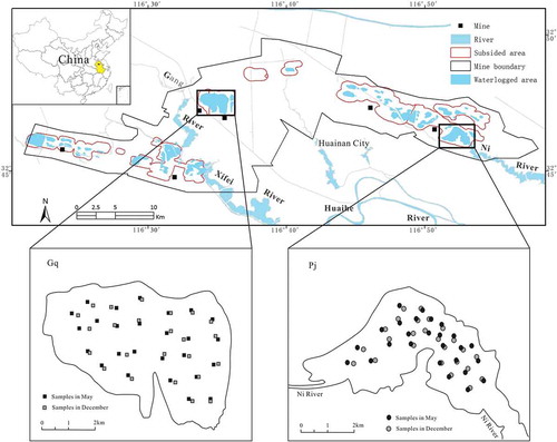
In this study, the Guqiao (Gq) and Panji (Pj) waterlogged areas were chosen for analysis as representative of the two main types of waterlogged area in this locality: closed and semi-closed. Both the areas are located in Huainan City, Anhui Province, East China (Figure 1), where there has been extensive underground coal mining for decades (Dong et al. 2013). The two waterlogged areas cover areas of 4.5 and 3.5 km², and have average depths of 4 m and 4.5 m, respectively. The two waterlogged areas are the sites of 2 districts, 5 towns, and nearly 30 villages with a total of ~100,000 inhabitants. Furthermore, two power plants and coal separating plants have been built close to Gq and Pj. The water quality in this area is therefore vulnerable to pollution from various sources, including industrial enterprises, farmland, and local residents. Gq, adjacent to the Gang River, started to form in 2003 in response to exploitation of the Guqiao coal mine. It is a closed waterlogged area and is strongly influenced by seasonal precipitation. Pj started to form in the 1980s in response to exploitation of the Panyi coal mine. It is semi-closed and is connected to the Ni River. Seasonal precipitation has a strong influence on the hydrological characteristics of the Ni River. Sediment loads may be high and bottom sediments may be re-suspended during the rainy season due to increased flow.

Figure 1. Location of the study area and sampling sites in Gq and Pj. Black filled symbols indicate samples collected in May; gray-filled symbols indicate samples collected in November. For full color versions of the figures in this paper, please see the online version.

Field data

Field data were collected at 52 stations (26 in Pj and 26 in Gq) from 21 to 22 May 2013 and at 49 stations (25 in Pj and 24 in Gq) from 16 to 17 November 2013. A standard set of water quality parameters was measured at each station, including water temperature (°C), pH, and water clarity (measured using a standard Secchi disk). Water samples were collected at a depth of 0.5 m with amber bottles and were immediately stored in a cooler containing ice packs. Information about the physicochemical and optical properties of the water samples collected is presented in Tables 1 and 2.

Table 1. Descriptive statistics of the water quality parameters measured in Pj.

		pH	T (°C)	Chl-a (mg m^−3)	SDD (m)	TSM (g m^−3)	ap(440) (m^−1)	ap(675) (m^−1)	ad(440) (m^−1)	aph(440) (m^−1)	aph(675) (m^−1)	aCDOM(440) (m^−1)
May (N = 26)	Min	7.93	25.6	10.62	0.43	3.4	1.01	0.42	0.57	0.66	0.32	0.67
	Max	8.55	27.7	45.06	0.89	16.5	2.76	0.91	1.45	1.81	0.75	2.15
	Mean	8.32	27.1	26.61	0.65	8.6	1.82	0.74	0.78	1.06	0.58	1.27
	SD	0.21	0.66	9.74	0.13	3.32	0.24	0.16	0.14	0.11	0.09	0.35
November (N = 25)	Min	7.97	17.7	2.11	0.41	1.24	1.43	0.39	0.69	0.51	0.25	0.69
	Max	8.32	19.3	13.89	0.63	8.25	2.54	0.83	1.66	0.94	0.55	2.44
	Mean	8.09	18.3	6.98	0.49	4.26	1.94	0.60	1.02	0.72	0.38	1.75
	SD	0.08	0.53	3.59	0.06	1.52	0.32	0.11	0.22	0.18	0.10	0.39

Note: Chl-a – Chlorophyll-a concentration, SDD – water clarity, TSM – concentration of total suspended mater, a_p(440) – absorption coefficient spectra of total particulate matter at 440 nm, a_p(675) – absorption coefficient spectra of total particulate matter at 675 nm, a_d(440) – absorption coefficient of nonpigment suspended matter at 440 nm, a_ph(440) – absorption coefficient of phytoplankton at 440 nm, a_ph(675) – absorption coefficient of phytoplankton at 675 nm, a_CDOM(440) – absorption coefficient of CDOM at 440 nm, N – number of samples.

Table 2. Descriptive statistics of the water quality parameters measured in Gq.

		pH	T (°C)	Chl-a (mg m^−3)	SDD (m)	TSM (g m^−3)	ap(440) (m^−1)	ap(675) (m^−1)	ad(440) (m^−1)	aph(440) (m^−1)	aph(675) (m^−1)	aCDOM(440) (m^−1)
May (N = 26)	Min	7.82	26.1	8.49	0.28	1.42	1.62	0.72	0.55	0.78	0.45	0.75
	Max	9.21	27.9	64.45	0.81	12.45	3.54	1.18	1.19	2.55	1.14	1.79
	Mean	8.49	27.3	34.76	0.56	6.02	2.07	1.01	0.72	1.59	0.83	1.22
	SD	0.32	0.61	14.39	0.20	2.28	0.52	0.24	0.32	0.57	0.48	0.27
November (N = 24)	Min	8.43	17.6	5.91	0.20	1.31	1.60	0.45	0.63	0.45	0.32	1.28
	Max	8.85	19.9	21.84	0.72	7.62	3.67	0.85	1.61	1.93	0.82	2.16
	Mean	8.55	18.5	13.63	0.41	3.49	2.49	0.67	1.09	0.91	0.51	1.68
	SD	0.11	0.57	5.60	0.17	1.87	0.67	0.37	0.43	0.31	0.30	0.36

Note: Chl-a – Chlorophyll-a concentration, SDD – water clarity, TSM – concentration of total suspended mater, a_p(440) – absorption coefficient spectra of total particulate matter at 440 nm, a_p(675) – absorption coefficient spectra of total particulate matter at 675 nm, a_d(440) – absorption coefficient of nonpigment suspended matter at 440 nm, a_ph(440) – absorption coefficient of phytoplankton at 440 nm, a_ph(675) – absorption coefficient of phytoplankton at 675 nm, a_CDOM(440) – absorption coefficient of CDOM at 440 nm, N – number of samples.

Water samples and remote sensing reflectance spectra were collected at the same time at each station, mostly between 10:00 and 14:00 local time. Field spectra were measured using a portable spectroradiometer (ASD FieldSpec) with a spectral range of 325–1075 nm and a spectral resolution of 3 nm. Water surface reflectance spectral data were measured following Mueller et al. (2003). The radiance spectra of a standard 30% gray reference panel (L_p), water (L_sw) at approximately 1 m above the water surface, and the sky (L_sky) were measured at each station. To avoid the influence of direct solar radiation and any interference between the boat and the water surface, the optical fiber was positioned at an azimuth angle of 90°–135° to the solar principal plane and at a zenith angle of 30°–40° (Li et al. 2012). After measuring the water radiance, the spectroradiometer was then rotated upwards by 90°–120° to measure the skylight radiance (L_sky). The view azimuth angle was the same as the angle used for measuring water radiance (L_sw). To optimize the signal-to-noise ratio and reduce errors in in situ measurements, the relevant spectra were measured 10 times at each sampling site. Remote sensing reflectance (R_rs(λ)) was calculated as follows:

(1)

where is the reflectance of skylight at the air–water interface, for which a constant of 0.0226 was used in this study. represents reflectance from the gray reflectance standard.

Laboratory analysis

Water samples on which Chl-a concentrations were determined were filtered with GF/C filters (Whatman). After overnight extraction in a dark freezer with 90% acetone, the samples were centrifuged for 5 min and spectrophotometrically analyzed at 750 and 665 nm. The Chl-a concentration was then calculated following Lorenzen (1967) and Chen, Chen, and Hu (2006). Concentrations of total suspended matter (TSM) were determined gravimetrically (Eaton et al. 2005). Water samples were filtered through pre-combusted GF/C filters (Whatman) to remove suspended organic matter; the filter papers were then dried and weighed (Tables 1 and 2). Water quality parameters for each sampling location were analyzed in triplicate to ensure accurate measurement.

The adsorption spectra of the water samples were determined, and values of the absorption coefficient spectra of CDOM [], total particulate matter [], phytoplankton [], and nonpigment suspended matter [] were calculated using the quantitative filter technique (QFT), employing the method proposed by Zhang et al (2009).

Prior to CDOM absorption measurements, samples were filtered through a 0.2 μm membrane filter into acid-washed and pre-combusted glass bottles. After filtration, CDOM absorbance was measured in a 1 cm quartz cell from 200 to 800 nm using a spectrophotometer, with Milli-Q water () as a reference. To avoid scattering and baseline fluctuations, the absorbance data were corrected by subtracting the mean value of the measured absorbance from 700 to 750 nm (Bricaud, Morel, and Prieur 1981; Babin et al. 2003). The value of was calculated as follows:

(2)

where is the absorption at wavelength (nm) and l is the path length (m). The CDOM spectral absorption was fitted to a nonlinear exponential function using a function form (Bricaud, Morel, and Prieur 1981):

(3)

where is the reference wavelength and is the measured absorption at the reference wavelength. In this case, the reference wavelength was 440 nm. is the absorption spectral slope coefficient of CDOM.

The absorption of total particulate matter was measured using a spectrophotometer after water samples were filtered through 0.7 μm Whatman GF/F filters. The absorbance of total particulate matter was recorded at 1 nm intervals from 350 to 800 nm, using a blank filter wetted with Milli-Q water as a reference. The absorption spectra were corrected for path length amplification (Mitchell 1990; Tassan and Ferrari 1995) and baseline offset by subtracting the average absorbance from 700 to 750 nm (Mitchell et al. 2002). The absorbance values were converted to a_p(λ) as follows:

(4)

where is the absorbance at wavelength , is the effective filtration area, and is the filtration volume.

The absorbance of nonpigmented suspended matter was measured after methanol extraction, in the same manner as . Values of were converted to using Equation (4). The spectral absorption coefficients of phytoplankton () were obtained by subtracting from :

(5)

The spectral absorption by nonpigmented suspended matter was fitted to a nonlinear exponential function using a function form (Bricaud, Morel, and Prieur 1981):

(6)

where is a reference wavelength and is the absorption measured at the reference wavelength. A reference wavelength of 440 nm was chosen. is the absorption spectral slope coefficient of nonpigmented suspended matter.

Accuracy assessment

The data collected in Pj and Gq were randomly divided into two independent subsets: one for model development and the other for model validation. The coefficient of determination (R²), the mean absolute percent error (MAPE) (7), and the root mean square error (RMSE) (8) were used to evaluate the accuracy of the different models, as follows:

(7)

(8)

where n is the number of samples, is the measured value, and is the estimated value.

Results

Variation in absorption coefficients

CDOM absorption increased exponentially toward the blue and ultraviolet (UV) wavelengths. The spectral curves and the mean spectral curves for the 400–750 nm range for May and November 2013 are presented in Figure 2d (for Pj) and Figure 3d (for Gq). There was high seasonal and spatial variability in the spectra of . The average in November was higher than that in May (Tables 1 and 2). Furthermore, the average in Pj (1.75 ± 0.39 m⁻¹ in November, 1.27 ± 0.35 m⁻¹ in May) was higher than that in Gq (1.68 ± 0.36 m⁻¹ in November, 1.22 ± 0.27 m⁻¹ in May) in both May and November.

Figure 2. Absorption spectra of (a) total particulate matter, (b) nonpigmented suspended matter, (c) phytoplankton, and (d) CDOM in Pj.

Figure 3. Absorption spectra of (a) total particulate matter, (b) nonpigment suspended matter, (c) phytoplankton, and (d) CDOM in Gq.

The spectral slope of CDOM absorption at 440 nm (), calculated between 400 and 600 nm, was varied from 0.0107 to 0.0197 nm⁻¹ in Pj and from 0.0119 to 0.0191 nm⁻¹ in Gq. The average values of in Pj showed little seasonal variation and were 0.0158 nm⁻¹ in May and 0.0145 nm⁻¹ in November. The average values of in Gq during May and November were 0.0166 and 0.0143 nm⁻¹, respectively.

The absorption coefficient of the nonpigmented suspended matter decreased as the wavelength increased from 400 to 750 nm in both Pj and Gq (Figures 2b and 3b). Values of showed considerable variation between May and November 2013 in both areas, and in Pj they varied from 0.57 to 1.45 m⁻¹ in May and from 0.69 to 1.66 m⁻¹ in November; in Gq they varied from 0.55 to 1.19 m⁻¹ in May and from 0.63 to 1.61 m⁻¹ in November. The variation might have resulted from an increase in organic materials from phytoplankton decomposition in November. The average values of were higher in Pj than in Gq. The spectral slope of was calculated between 400 and 600 nm. Similar to , showed considerable temporal variation, and in Pj ranged from 0.01128 to 0.01147 nm⁻¹ in May and from 0.01123 to 0.01174 nm⁻¹ in November; in Gq they varied from 0.01131 to 0.01145 nm⁻¹ in May and from 0.01138 to 0.01169 nm⁻¹ in November. These values of are influenced by inorganic or mineral-dominated sediments (Bowers, Harker, and Stephan 1996; Babin et al. 2003).

The spectra obtained during the cruises in Pj and Gq showed two diagnostic absorption peaks: one in the blue wavelength and one in the red wavelength (Figures 2c and 3c). The value varied markedly in space and time. In May, values of at 440 and 675 nm ranged from 0.66 to 1.81 m⁻¹ and from 0.32 to 0.75 m⁻¹ in Pj, and from 0.78 to 2.55 m⁻¹ and 0.45 to 1.14 m⁻¹ in Gq, respectively. In November, these values ranged from 0.51 to 0.94 m⁻¹ and from 0.25 to 0.55 m⁻¹ in Pj, and from 0.45 to 1.93 m⁻¹ and from 0.32 to 0.82 m⁻¹ in Gq, respectively. The mean values of and were higher in May than in November (Tables 1 and 2). Furthermore, the mean values of at 440 and 675 nm were higher in Gq (1.21 ± 0.53 in May and 0.71 ± 0.31 in November) than in Pj (0.82 ± 0.1 in May and 0.55 ± 0.14 in November).

Inland waters have multiple bio-optical properties, and are generally dominated by one or more of their inherent optical properties (IOPs), such as phytoplankton, nonpigmented suspended matter, and CDOM (Li et al. 2012). Ternary plots were constructed to illustrate the dominant absorbing constituents in Pj and Gq (Figure 4). These two waterlogged areas were significantly influenced by nonpigmented components (a_d(λ) and a_CDOM(λ)), which were important absorbers of light in the blue part of the spectrum; their contributions to total nonwater absorption at 440 nm were more than 50% in May and 60% in November. However, their contributions decreased to 40% at 675 nm because of the exponential decrease in a_d(λ) and a_CDOM(λ) with increasing wavelength (Naik et al. 2011). In contrast, the phytoplankton absorption contribution increased as the wavelength increased and generally dominated at 675 nm. Phytoplankton absorption in Pj and Gq exceeded 60% in May and November, and accounted for as much as 80–90% of the total nonwater absorption at some stations in Gq. Further, Spearman correlation analysis (r_s) indicated a stronger relationship between and Chl-a (r_s = 0.66 in Pj; r_s = 0.69 in Gq) (Figure 5) than between and Chl-a (r_s = 0.47 in Pj; r_s = 0.51 in Gq). These results highlight the important role of the red spectral region in the development of a model for Chl-a estimation in waters with high CDOM and high absorption by nonpigmented suspended matter.

Figure 4. Ternary plots showing the relative contributions by CDOM (), phytoplankton () and nonpigmented suspended matter () to total absorption at (a) 440 nm and (b) 675 nm.

Figure 5. Relationships between a_ph(675) and Chl-a in (a) Pj and (b) Gq.

Reflectance spectral characteristics of Chl-a

The reflectance spectra collected in Pj and Gq showed optical conditions typical of turbid productive inland waters (Figure 6). In the blue spectral region, the combined absorption by phytoplankton, nonpigmented suspended matter, and CDOM absorption resulted in a low sensitivity to variations in Chl-a concentrations (Gurlin, Gitelson, and Moses 2011; Zhang et al. 2009). The first reflectance peak emerged around 570 nm, which has previously been attributed to backscattering by particles (Lubac and Loisel 2007). There was a distinct reflectance feature in the vicinity of 675 nm, corresponding to the maximum Chl-a absorption (Bidigare et al. 1990). However, the reflectance in this range was also influenced by absorption and scattering of other constituents, which may have weakened the correlation between R_rs(675) and Chl-a (Zimba and Gitelson 2006; Zhang et al. 2009). The second reflectance peak appeared around 700 nm and was caused by the combined effects of reduced Chl-a absorption and pure water (Bricaud et al. 1995; Gitelson et al. 2008; Gilerson et al. 2010). This spectral region included the Chl-a fluorescence emission peak, the magnitude of which varied widely between moderate and high Chl-a concentrations (Gitelson et al. 2008). Furthermore, the position of the reflectance peak near 700 nm was red-shifted as the Chl-a concentration increased in Gq. In the NIR region, Chl-a absorption decreased with increasing wavelength, whereas absorption of pure water increased (Gitelson, Schalles, and Hladik 2007). The high reflectance in this region was caused by interference from other water constituents.

Figure 6. Reflectance spectra collected in (a) Pj and (b) Gq.

Models for estimating Chl-a concentration

The optimal spectral bands of Chl-a retrieval models may be different in waters with different optical properties (Koponen et al. 2002; Gitelson, Schalles, and Hladik 2007; Gitelson et al. 2009; Zhang et al. 2011). Therefore, it is important to establish specific Chl-a retrieval models for specific water optical characteristics. The NIR-red, three-band, and NDCI models were established to obtain accurate information about variations in the Chl-a concentrations in Pj and Gq, and were calibrated using in situ hyperspectral data. The optimal spectral bands for the NIR-red model were determined using the optimization technique of Gitelson, Schalles, and Hladik (2007). The most sensitive band ratios, R_rs(692)/R_rs(675) and R_rs(706)/R_rs(680), were selected to estimate the Chl-a concentrations in Pj and Gq, respectively (Figure 7(a, b)), where R_rs(692) and R_rs(706) were close to the average position of the reflectance peak in the NIR region, and R_rs(675) and R_rs(680) were close to the maximum Chl-a absorption. The NIR-red model, which has been used successfully in many inland water bodies since being proposed by Gitelson, Keydan, and Shishkin (1985), accurately estimated the Chl-a concentrations in this study. Figure 7(a, b) shows a reasonable linear relationship between the NIR-red model and Chl-a in Pj (R² = 0.80), but that there was a polynomial relationship between this model and Chl-a in Gq (R² = 0.82).

Figure 7. Three models for estimating Chl-a concentrations: (a) NIR-red model in Pj, (b) NIR-red model in Gq, (c) three-band model in Pj, (d) three-band model in Gq, (e) NDCI model in Pj, and (f) NDCI model in Gq.

The optimization approach described earlier for the NIR-red model was used to determine the optimal spectral bands for the three-band model. The initial positions for λ₁ and λ₃ were set at 660 and 750 nm, respectively, to search for the optimal position of λ₂. The optimal position for λ₂ and the initial position for λ₃ were then used to determine the optimal position for λ₁. Subsequently, the optimal positions obtained for λ₁ and λ₂ were selected to determine the optimal position of λ₃. Finally, wavelengths at 665, 698, and 743 nm were selected as the optimal positions for the three-band model in Pj, while wavelengths at 671, 706, and 748 nm were selected as the optimal positions for the three-band model in Gq (Figure 7(c, d)). The performance of the three-band model was superior to that of the NIR-red model. The three-band model showed a polynomial relationship with Chl-a in Pj (R² = 0.87) and a strong linear relationship with Chl-a in Gq (R² = 0.88).

The optimal spectral bands for developing the NDCI were selected from the absorption peak near 675 nm and the reflectance peak near 700 nm, as these spectral bands are most sensitive to variations in Chl-a in water (Mishra and Mishra 2012). Application of the optimization technique showed that the optimal spectral bands for developing the NDCI in Pj and Gq were at 675 and 692 nm and at 680 and 706 nm, respectively. The NDCI showed a strong polynomial relationship with Chl-a concentrations in Gq (R² = 0.90; Figure 7f), and a relatively weak polynomial relationship with Chl-a concentrations in Pj (R² = 0.84; Figure 7e).

Model validation

To comprehensively evaluate the performance of the three Chl-a estimation models in Pj and Gq, the independent validation data (n = 17 for Pj and n = 16 for Gq) were used to validate the models by retrieving the MAPE and RMSE values for Chl-a (Figure 8). The NIR-red model reported an MAPE of 20.05% in Pj and 19.35% in Gq, and an RMSE of 6.13 mg m⁻³ in Pj and 5.52 mg m⁻³ in Gq. The results from the three-band model were better than those from the NIR-red model. The three-band model yielded MAPE values of 11.35% and 11.16% when applied to Pj and Gq, respectively, and RMSE values of 3.87 and 3.28 mg m⁻³ in Pj and Gq, respectively. The NDCI model, with an MAPE value of 10.88% and an RMSE value of 3.19 mg m⁻³, yielded more accurate results for Gq than the three-band model, but gave relatively low-accuracy results for Pj, for which the MAPE was 14.52% and the RMSE was 4.69 mg m⁻³. Of note, the Chl-a concentrations were significantly and systematically overestimated by all three models, possibly because of absorption of nonpigmented suspended matter (Gons et al. 2000).

Figure 8. Validation of the estimated Chl-a concentrations with measured Chl-a concentrations: (a) NIR-red model in Pj, (b) NIR-red model in Gq, (c) three-band model in Pj, (d) three-band model in Gq, (e) NDCI model in Pj, and (f) NDCI model in Gq.

Discussion

The results of in situ monitoring show that the Chl-a concentrations were higher in May (26.61 ± 9.74 mg m⁻³ in Pj; 34.76 ± 14.39 mg m⁻³ in Gq) than in November, corresponding to the timing of obvious algal blooms in some waters. However, Chl-a concentrations were still relatively high in November (6.98 ± 3.59 mg m⁻³ in Pj; 13.63 ± 5.6 mg m⁻³ in Gq), demonstrating that Pj and Gq were eutrophic. Chl-a concentrations were higher in Gp than in Pj because of nutrient accumulation in closed water, which results in the rapid growth of algae. Similarly, the TSM concentrations were significantly higher in both Pj and Gq in May than in November, as a result of the noticeable sediment re-suspension by considerable rain-generated turbulence in May during the rainy season. TSM concentrations were higher in Pj than in Gq due to the influence of the Ni River. Rivers can transport large quantities of sediment particles, and elevated flows can cause the re-suspension of bottom sediments, especially in the rainy season. Furthermore, Chl-a concentrations and TSM concentrations were positively correlated in Gq, but no relationship was found in Pj. This result indicates a strong interdependence between Chl-a and TSM in the closed water because of the frequent algal blooms that make a large contribution to TSM (Li et al. 2012).

There was considerable variation in the concentrations and spectral absorption coefficients of the three optically active substances in Pj and Gq. The contributions of the nonpigmented components and were higher in Pj than in Gq because of the influence of the Ni River. The Ni River transports large quantities of humic substances and dissolved organic matter, which drive much of the variability in the nonpigmented suspended matter and CDOM absorption. Water flow and the hydrological properties of the water column have a strong influence on the IOPs through modifications of the package effect and the accumulation of suspended material (Bricaud et al. 2004). In contrast, the values of were higher in Gq than in Pj, which corresponds with the higher Chl-a concentrations in Gq.

In this study, in situ hyperspectral data were used to retrieve the concentrations of Chl-a in waterlogged areas in Huainan. All three models gave good estimations of Chl-a concentrations in Pj and Gq. The three-band model and the NDCI model yielded higher R² values and lower RMSE values than the NIR-red model. Moreover, the accuracy of the NDCI model was highest in Gq. Comparison with an earlier study by Mishra (Mishra and Mishra 2012) shows that the optimal spectral band λ₁ of the NDCI model shifted from 665 to 675 nm (Pj) and from 665 to 680 nm (Gq) because of the high Chl-a concentrations in the waterlogged areas. Furthermore, in the waterlogged areas the optimal spectral bands were influenced not only by Chl-a, but also by TSM and CDOM. In contrast, the accuracy of the three-band model was highest in Pj. The optimal spectral bands of the three-band model for the waterlogged areas were within the ranges recommended by previous studies (Gitelson, Schalles, and Hladik 2007; Gitelson et al. 2008). One of the reasons for the superior performance of the three-band model was the removal of interference from backscattering (Zhang et al. 2009). These results indicate that the NDCI model was more suitable for the relatively low TSM and high Chl-a concentrations in the closed waterlogged area, and that the three-band model was more suitable for the relatively high TSM and low Chl-a concentrations in the semi-closed waterlogged area.

The present results indicate the potential of in situ hyperspectral data for monitoring Chl-a concentrations in waterlogged area. In addition, the model and method discussed in this paper may play an important role in estimating Chl-a concentrations for water quality monitoring and water resource management in other waterlogged areas in China and worldwide. This applies not only to waterlogged areas caused by underground coal mining in Xuzhou (Du et al. 2007), Huaibei (Fan et al. 2012), and Yanzhou (Hu, Xu, and Zhao 2012), which have similar environmental conditions to those at Huainan, but also to waterlogged areas caused by uneven irrigation and over-irrigation in India (Goyal and Arora 2012; Singh, Kumar, and Mathur 2013), Bangladesh (Adri and Islam 2012) and elsewhere.

Although hyperspectral satellite remote sensing data are not appropriate for small waterlogged areas, due to poor spatial resolution, upcoming satellite sensors with higher spatial and spectral resolutions such as Sentinels, HyspIRI, and GEO-CAPE may be appropriate for such areas. These new missions will not only fill a gap in data provision that has existed since previous missions ended, but will result in a step-change in the use of satellite observations for monitoring the quality of inland water bodies. The combination of hyperspectral satellite data with finer spatial resolution and in situ hyperspectral data will enhance the applicability and robustness of Chl-a retrieval models for waterlogged areas. It will also provide a better understanding of the spatiotemporal distribution of water quality parameters and help to predict future changes in water quality in waterlogged areas.

Conclusions

Remote sensing techniques were used to estimate the concentrations of Chl-a in waterlogged areas that developed as a result of long-term underground coal mining. The Gq and Pj waterlogged areas were chosen as representative examples of the two main types of waterlogged area, closed and semi-closed. There was significant difference between Pj and Gq in terms of the spectral absorption coefficients of the three optically active substances, (a_ph(λ), a_d(λ), and a_CDOM(λ)). These two waterlogged areas were significantly influenced by nonpigmented components (a_d(λ) and a_CDOM(λ)). The contributions from nonpigmented components were higher in Pj than in Gq because of the connection to the Ni River.

The NIR-red, three-band, and NDCI models were calibrated and validated for estimating Chl-a concentrations using in situ hyperspectral datasets. All three models gave good estimations of Chl-a concentrations in Pj and Gq, which indicates that hyperspectral remote sensing data, based on field spectral measurements, can be used for estimating Chl-a concentrations in waterlogged areas. Furthermore, the three-band model is more accurate for semiclosed waterlogged areas, while the NDCI model is more accurate for closed waterlogged areas.

Disclosure statement

No potential conflict of interest was reported by the authors.

Acknowledgments

The authors thank Gao Liangmin, Li Shaopengm, and Ye Yuanyuan for their assistance in sample collection and laboratory analysis. The authors are grateful to anonymous reviewers for constructive comments and recommendations that improved an earlier version of the manuscript.

Additional information

Funding

This work was supported by the National Key Technology R&D Program [No. 2012BAC10B02]; Huainan Mining Group [No. HNKY-JT-JS-(2013)-004].

References

- Adri, N., and I. Islam. 2012. “Vulnerability and Coping Strategies in Waterlogged Area: A Case Study from Keshabpu, Bangladesh.” International Journal of Environment 2 (1): 48–56.
- Baban, S. M. 1996. “Trophic Classification and Ecosystem Checking of Lakes Using Remotely Sensed Information.” Hydrological Sciences Journal 41 (6). doi:939-957.doi:10.1080/02626669609491560.
- Babin, M., D. Stramaski, G. M. Ferrari, H. Claustre, A. Bricaud, G. Obolensky, and N. Hoepffner. 2003. “Variations in the Light Absorption Coefficients of Phytoplankton, Non-Algal Particles, and Dissolved Organic Matter in Coastal Waters around Europe.” Journal of Geophysical Research 108: 3211. doi:10.1029/2001jc000882.
- Bidigare, R. R., M. E. Ondrusek, J. H. Morrow, and D. A. Kiefer. 1990. “In-Vivo Absorption Properties of Algal Pigments.” In International Society for Optics and Photonics. Ocean Optics X, September 1, Vol. 1302, 290–302. doi:10.1117/12.21451.
- Bowers, D. G., G. E. L. Harker, and B. Stephan. 1996. “Absorption Spectra of Inorganic Particles in the Irish Sea and Their Relevance to Remote Sensing of Chlorophyll.” International Journal of Remote Sensing 17 (12): 2449–2460. doi:10.1080/01431169608948782.
- Bricaud, A., M. Babin, A. Morel, and H. Claustre. 1995. “Variability in the Chlorophyll-Specific Absorption Coefficients of Natural Phytoplankton: Analysis and Parameterization.” Journal of Geophysical Research: Oceans (1978–2012) 100 (C7): 13321–13332. doi:10.1029/95JC00463.
- Bricaud, A., H. Claustre, J. Ras, and K. Oubelkheir. 2004. “Natural Variability of Phytoplanktonic Absorption in Oceanic Waters: Influence of the Size Structure of Algal Populations.” Journal of Geophysical Research: Oceans (1978–2012) 109 (C11). doi:10.1029/2004JC002419.
- Bricaud, A., A. Morel, and L. Prieur. 1981. “Absorption by Dissolved Organic Matter of the Sea (Yellow Substance) in the UV and Visible Domains.” Limnology Oceanography 26: 43–53. doi:10.4319/lo.1981.26.1.0043.
- Chen, Y., K. Chen, and Y. Hu. 2006. “Discussion on Possible Error for Phytoplankton Chlorophyll-A Concentration Analysis Using Hot-Ethanol Extraction Method.” Journal of Lake Sciences 18 (5): 550–552. [In Chinese]. doi:10.18307/2006.0519
- Dall’Olmo, G., and A. A. Gitelson. 2005. “Effect of Bio-Optical Parameter Variability on the Remote Estimation of Chlorophyll-A Concentration in Turbid Productive Waters: Experimental Results.” Applied Optics 44 (3): 412–422. doi:10.1364/AO.44.000412.
- Dall’Olmo, G., A. A. Gitelson, and D. C. Rundquist. 2003. “Towards a Unified Approach for Remote Estimation of Chlorophyll-A in Both Terrestrial Vegetation and Turbid Productive Waters.” Geophysical Research Letters 30 (18): 1938. doi:10.1029/2003GL018065.
- Dekker, A. G. 1993. “Detection of optical water quality parameters for eutrophic waters by high resolution remote sensing.” PhD Thesis, Free University, Amsterdam, The Netherlands.
- Dong, S., S. Samsonov, H. Yin, S. Yao, and C. Xu. 2014. “Spatio-Temporal Analysis of Ground Subsidence Due to Underground Coal Mining in Huainan Coalfield, China.” Environment Earth Sciences. ( accepted). doi:10.1007/s12665-014-3806-4.
- Dong, S., H. Yin, S. Yao, and F. Zhang. 2013. “Detecting Surface Subsidence in Coal Mining Area Based on Dinsar Technique.” Journal of Earth Science 24: 449–456. doi:10.1007/s12583-013-0342-1.
- D’Sa, E. J. 2014. “Assessment of Chlorophyll Variability along the Louisiana Coast Using Multi-Satellite Data.” GIScience & Remote Sensing 51 (2): 139–157. doi:10.1080/15481603.2014.895578.
- Du, P., H. Zhang, P. Liu, K. Tan, and Z. Yin. 2007. “Land Use/Cover Change in Mining Areas Using Multi-Source Remotely Sensed Imagery.” IEEE International Workshop on Analysis of Multi-Temporal Remote Sensing images, Leuven, 1–7. doi:10.1109/MULTITEMP.2007.4293074.
- Duan, H., R. Ma, S. G. Simis, and Y. Zhang. 2012. “Validation of MERIS Case-2 Water Products in Laketaihu, China.” Giscience & Remote Sensing 49 (6): 873–894. doi:10.2747/1548-1603.49.6.873.
- Duan, H., Y. Zhang, B. Zhang, K. Song, Z. Wang, D. Liu, and F. Li. 2008. “Estimation of Chlorophyll-A Concentration and Trophic States for Inland Lakes in Northeast China from Landsat TM Data and Field Spectral Measurements.” International Journal of Remote Sensing 29 (3): 767–786. doi:10.1080/01431160701355249.
- Eaton, A. D., L. S. Clesceri, E. W. Rice, A. E. Greenberg, and M. A. H. Franson. 2005. APHA: Standard Methods for the Examination of Water and Wastewater. 21st ed. Washington, DC: American Public Health Association.
- Fan, T. G., J. P. Yan, S. Wang, and S. X. Ruan. 2012. “The Environment and the Utilization the Status of the Subsidence Area in the Xu Zhou, Yan Zhou and Huainan and Huaibei Region of China.” AGH Journal of Mining and Geoengineering 36: 127–133. doi:10.7494/mining.2012.36.3.127.
- Gilerson, A. A., A. A. Gitelson, J. Zhou, D. Gurlin, W. Moses, I. Ioannou, and S. A. Ahmed. 2010. “Algorithms for Remote Estimation of Chlorophyll-A in Coastal and Inland Waters Using Red and Near Infrared Bands.” Optics Express 18 (23): 24109–24125. doi:10.1364/OE.18.024109.
- Gitelson, A., G. Keydan, and V. Shishkin. 1985. “Inland Waters Quality Assessment from Satellite Data in Visible Range of the Spectrum.” Soviet Remote Sensing 6: 28–36.
- Gitelson, A. A., G. Dall’Olmo, W. Moses, D. C. Rundquist, T. Barrow, T. R. Fisher, and D. Gurlin. 2008. “A Simple Semi-Analytical Model for Remote Estimation of Chlorophyll-A in Turbid Waters: Validation.” Remote Sensing of Environment 112 (9): 3582–3593. doi:10.1016/j.rse.2008.04.015.
- Gitelson, A. A., D. Gurlin, W. J. Moses, and T. Barrow. 2009. “A Bio-Optical Algorithm for the Remote Estimation of the Chlorophyll-A Concentration in Case 2 Waters.” Environmental Research Letters 4 (4): 045003. doi:10.1088/1748-9326/4/4/045003.
- Gitelson, A. A., J. F. Schalles, and C. M. Hladik. 2007. “Remote Chlorophyll-A Retrieval in Turbid, Productive Estuaries: Chesapeake Bay Case Study.” Remote Sensing of Environment 109 (4): 464–472. doi:10.1016/j.rse.2007.01.016.
- Gons, H. J., M. Rijkeboer, S. Bagheri, and K. G. Ruddick. 2000. “Optical Teledetection of Chlorophyll a in Estuarine and Coastal Waters.” Environmental Science & Technology 34 (24): 5189–5192. doi:10.1021/es0012669.
- Gons, H. J., M. Rijkeboer, and K. G. Ruddick. 2002. “A Chlorophyll-Retrieval Algorithm for Satellite Imagery (Medium Resolution Imaging Spectrometer) of Inland and Coastal Waters.” Journal of Plankton Research 24 (9): 947–951. doi:10.1093/plankt/24.9.947.
- Goyal, A. N. A. R., and A. N. Arora. 2012. “Predictive Modelling of Groundwater Flow of Indira Gandhi Nahar Pariyojna, Stage I.” Ish Journal of Hydraulic Engineering 18 (2): 119–128. doi:10.1080/09715010.2012.695447.
- Gurlin, D., A. A. Gitelson, and W. J. Moses. 2011. “Remote Estimation of Chl-A Concentration in Turbid Productive Waters—Return to a Simple Two-Band Nir-Red Model?” Remote Sensing of Environment 115 (12): 3479–3490. doi:10.1016/j.rse.2011.08.011.
- He, C., H. Liu, and H. Gui. 2005. “Environment Evaluation on Typical Water Area Resulting from Coal-Mine Subsidence in Huainan.” Journal of China Coal Society 30 (6): 754–758.
- Hu, Z., and X. Wu. 2013. “Optimization of Concurrent Mining and Reclamation Plans for Single Coal Seam: A Case Study in Northern Anhui, China.” Environment Earth Sciences 68: 1247–1254. doi:10.1007/s12665-012-1882-9.
- Hu, Z., X. Xu, and Y. Zhao. 2012. “Dynamic Monitoring of Land Subsidence in Mining Area from Multi-Source Remote-Sensing Data–A Case Study at Yanzhou, China.” International Journal of Remote Sensing 33 (17): 5528–5545. doi:10.1080/01431161.2012.663113.
- Huang, C., J. Zou, Y. Li, H. Yang, K. Shi, J. Li, Y. Wang, X. Chena, and F. Zheng. 2014. “Assessment of Nir-Red Algorithms for Observation of Chlorophyll-A in Highly Turbid Inland Waters in China.” ISPRS Journal of Photogrammetry and Remote Sensing 93: 29–39. doi:10.1016/j.isprsjprs.2014.03.012.
- Hui, G. 2013. “Management of Water Quality Information in Mining Subsidence Waterlogged Area.” Advanced Materials Research 726–731: 3702–3705. doi:10.4028/www.scientific.net/AMR.726-731.3702.
- Kallio, K., T. Kutser, T. Hannonen, S. Koponen, J. Pulliainen, J. Vepsäläinen, and T. Pyhälahti. 2001. “Retrieval of Water Quality from Airborne Imaging Spectrometry of Various Lake Types in Different Seasons.” Science of the Total Environment 268 (1–3): 59–77. doi:10.1016/S0048-9697(00)00685-9.
- Kim, Y. H., J. Im, H. K. Ha, J.-K. Choi, and S. Ha. 2014. “Machine Learning Approaches to Coastal Water Quality Monitoring Using GOCI Satellite Data.” GIScience & Remote Sensing 51 (2): 158–174. doi:10.1080/15481603.2014.900983.
- Koponen, S., J. Pulliainen, K. Kallio, and M. Hallikainen. 2002. “Lake Water Quality Classification with Airborne Hyperspectral Spectrometer and Simulated MERIS Data.” Remote Sensing of Environment 79 (1): 51–59. doi:10.1016/S0034-4257(01)00238-3.
- Le, C., Y. Li, Y. Zha, D. Sun, C. Huang, and H. Zhang. 2011. “Remote Estimation of Chlorophyll a in Optically Complex Waters Based on Optical Classification.” Remote Sensing of Environment 115 (2): 725–737. doi:10.1016/j.rse.2010.10.014.
- Li, L., R. E. Sengpiel, D. L. Pascual, L. P. Tedesco, J. S. Wilson, and E. Soyeux. 2010. “Using Hyperspectral Remote Sensing to Estimate Chlorophyll-A and Phycocyanin in a Mesotrophic Reservoir.” International Journal of Remote Sensing 31 (15): 4147–4162. doi:10.1080/01431161003789549.
- Li, Y., Q. Wang, C. Wu, S. Zhao, X. Xu, Y. Wang, and C. Huang. 2012. “Estimation of Chlorophyll a Concentration Using Nir/Red Bands of MERIS and Classification Procedure in Inland Turbid Water.” IEEE Transactions on Geoscience and Remote Sensing 50 (3): 988–997. doi:10.1109/TGRS.2011.2163199.
- Lorenzen, C. J. 1967. “Determination of Chlorophyll and Phaeopigments: Spec-Trophotometric Equations, Limnol.” Oceanography 12: 343–346.
- Lubac, B., and H. Loisel. 2007. “Variability and Classification of Remote Sensing Reflectance Spectra in the Eastern English Channel and Southern North Sea.” Remote Sensing of Environment 110 (1): 45–58. doi:10.1016/j.rse.2007.02.012.
- Ma, R., and J. Dai. 2005. “Investigation of Chlorophyll-A and Total Suspended Matter Concentrations Using Landsat ETM and Field Spectral Measurement in Taihu Lake, China.” International Journal of Remote Sensing 26 (13): 2779–2795. doi:10.1080/01431160512331326648.
- Mishra, D. R., B. A. Schaeffer, and D. Keith. 2014. “Performance Evaluation of Normalized Difference Chlorophyll Index in Northern Gulf of Mexico Estuaries Using the Hyperspectral Imager for the Coastal Ocean.” GIScience & Remote Sensing 51 (2): 175–198. doi:10.1080/15481603.2014.895581.
- Mishra, S., and D. R. Mishra. 2012. “Normalized Difference Chlorophyll Index: A Novel Model for Remote Estimation of Chlorophyll-A Concentration in Turbid Productive Waters.” Remote Sensing of Environment 117: 394–406. doi:10.1016/j.rse.2011.10.016.
- Mitchell, B. G., M. Kahru, J. Wieland, and M. Stramska. 2002. “Determination of Spectral Absorption Coefficients of Particles, Dissolved Material and Phytoplankton for Discrete Water Samples.” Ocean Optics Protocols for Satellite Ocean Color Sensor Validation, Revision 3: 231–257.
- Mitchell, G. 1990. “Algorithms for Determining the Absorption Coefficient for Aquatic Particulates Using the Quantitative Filter Technique (QFT).” Proceedings of the SPIE 1302: 137–148. doi:10.1117/12.21440.
- Mueller, J. L., G. S. F. C. R. McClain, J. L. Mueller, R. R. Bidigare, C. Trees, W. M. Balch, and L. Van. 2003. “Ocean Optics Protocols for Satellite Ocean Color Sensor Validation, Revision 5, Volume V: Biogeochemical and Bio-Optical Measurements and Data Analysis Protocols.” NASA Technical Memo 211621: 36.
- Naik, P., E. J. D’Sa, M. Grippo, R. Condrey, and J. Fleeger. 2011. “Absorption Properties of Shoal-Dominated Waters in the Atchafalaya Shelf, Louisiana, USA.” International Journal of Remote Sensing 32 (15): 4383–4406. doi:10.1080/01431161.2010.486807.
- Navalgund, R. R., V. Jayaraman, and P. S. Roy. 2007. “Remote Sensing Applications: An Overview.” Current Science 93 (12): 1747–1766.
- Palmer, S. C., T. Kutser, and P. D. Hunter. 2015. “Remote Sensing of Inland Waters: Challenges, Progress and Future Directions.” Remote Sensing of Environment 157: 1–8. doi:10.1016/j.rse.2014.09.021.
- Salas, E. A. L., and G. M. Henebry. 2009. “Area between Peaks Feature in the Derivative Reflectance Curve as a Sensitive Indicator of Change in Chlorophyll Concentration.” Giscience & Remote Sensing 46 (3): 315–328. doi:10.2747/1548-1603.46.3.315.
- Singh, P., V. Kumar, and A. Mathur. 2013. “A Comparative Study of Sodic Wastelands and Water logged Area Using IRS P6 LISS-III and LISS IV Data through the GIS Techniques.” International Journal of Engineering Research and Technology 2 (9): 1628–1639.
- Song, K., D. Lu, L. Li, S. Li, Z. Wang, and J. Du. 2012. “Remote Sensing of Chlorophyll-A Concentration for Drinking Water Source Using Genetic Algorithms (Ga)-Partial Least Square (PLS) Modeling.” Ecological Informatics 10: 25–36. doi:10.1016/j.ecoinf.2011.08.006.
- Sun, D., Y. Li, C. Le, K. Shi, C. Huang, S. Gong, and B. Yin. 2013. “A Semi-Analytical Approach for Detecting Suspended Particulate Composition in Complex Turbid Inland Waters (China).” Remote Sensing of Environment 134: 92–99. doi:10.1016/j.rse.2013.02.024.
- Tassan, S., and G. M. Ferrari. 1995. “An Alternative Approach to Absorption Measurements of Aquatic Particles Retained on Filters.” Limnology and Oceanography 40: 1358–1368. doi:10.4319/lo.1995.40.8.1358.
- Vincent, R. K., X. Qin, R. M. L. McKay, J. Miner, K. Czajkowski, J. Savino, and T. Bridgeman. 2004. “Phycocyanin Detection from LANDSAT TM Data for Mapping Cyanobacterial Blooms in Lake Erie.” Remote Sensing of Environment 89 (3): 381–392. doi:10.1016/j.rse.2003.10.014.
- Yan, J. P., Z. G. Zhao, G. Q. Xu, Y. B. Hu, G. M. Ma, R. Dong, and X. D. Liu. 2004. “Comprehensive Reclaimed Land Resources from Mining Subsidence Area of Huainan Mining Area.” Coal Science and Technology 32 (10): 56–58. [In Chinese].
- Yang, W., B. Matsushita, J. Chen, and T. Fukushima. 2011. “Estimating Constituent Concentrations in Case II Waters from MERIS Satellite Data by Semi-Analytical Model Optimizing and Look-Up Tables.” Remote Sensing of Environment 115 (5): 1247–1259. doi:10.1016/j.rse.2011.01.007.
- Zhang, Y., H. Lin, C. Chen, L. Chen, B. Zhang, and A. A. Gitelson. 2011. “Estimation of Chlorophyll-A Concentration in Estuarine Waters: Case Study of the Pearl River Estuary, South China Sea.” Environmental Research Letters 6 (2): 024016. doi:10.1088/1748-9326/6/2/024016.
- Zhang, Y., M. Liu, B. Qin, H. J. Van Der Woerd, J. Li, and Y. Li. 2009. “Modeling Remote-Sensing Reflectance and Retrieving Chlorophyll-A Concentration in Extremely Turbid Case-2 Waters (Lake Taihu, China).” IEEE Transactions on Geoscience and Remote Sensing 47 (7): 1937–1948. doi:10.1109/TGRS.2008.2011892.
- Zimba, P. V., and A. A. Gitelson. 2006. “Remote Estimation of Chlorophyll Concentration in Hyper-Eutrophic Aquatic Systems: Model Tuning and Accuracy Optimization.” Aquaculture 256: 272–286. doi:10.1016/j.aquaculture.2006.02.038.