A geostatistical temporal mixture analysis approach to address endmember variability for estimating regional impervious surface distributions

Abstract

Spectral mixture analysis (SMA) is a major approach for estimating fractional land covers through modeling the relationship between the spectral signatures of a mixed remote sensing pixel and those of the comprised pure land covers (also termed as endmembers). When SMA is implemented, endmember variability has proven to have significant impact on the accuracy of land cover fraction estimates. To address the endmember variability problem, this article developed a geostatistical temporal mixture analysis (GTMA) technique, with which spatially varying per-pixel endmember sets were estimated using an ordinary kriging interpolation technique. The method was applied to time-series moderate-resolution imaging spectroradiometer normalized difference vegetation index imagery in Wisconsin and North Carolina, United States to estimate regional impervious surface distributions. Analysis of results suggests that GTMA has achieved a promising accuracy. Detailed analysis indicates that a better performance has been achieved in less-developed areas than developed areas, and slight underestimation and slight overestimation have been detected in developed areas and less-developed areas, respectively. Moreover, while the performance of GTMA is comparable to those of phenology-based TMA and phenology-based multiple endmember TMA over the entire study area and in less-developed areas, a much better performance has been achieved in developed areas. Finally, this article argues that endmember variability may be more essential in developed areas when compared to less-developed areas.

Keywords:

• ordinary kriging
• endmember variability
• temporal mixture analysis
• impervious surfaces

1. Introduction

Spectral mixture analysis (SMA) is one of the major approaches for estimating fractional land covers through modeling the relationship between the spectral signatures of a mixed pixel and those of the comprised pure land covers (also termed as endmembers) within the pixel (Keshava 2003). Because of its effectiveness in addressing the mixed pixel problem, SMA has been applied in many fields, including urban impervious surface and vegetation mapping, agricultural production assessment, terrestrial ecosystem monitoring, geological mapping, etc. (Bedini 2009; Cunningham et al. 2015; Eckmann et al. 2010; Gilabert, Garcı́a-Haro, and Meliá 2000; Hestir et al. 2008; Jia et al. 2006; Johnson et al. 1993; Lelong, Pinet, and Poilvé 1998; Li et al. 2013; Liu et al. 2008; Rhee, Park, and Lu 2014; Rosa and Wiesmann 2013; Wu 2004; Wu and Murray 2003). When implementing SMA, the first and most important issue is the selection of endmember class types, number, and their corresponding spectra (Elmore et al. 2000; Tompkins et al. 1997). The set of corresponding spectra of endmember classes has been typically identified manually or statistically through analyzing the spectral plots. Subsequently, these endmembers were applied to each individual pixel of an image to extract areal fractions of land covers using spectral unmixing (Sabol, Adams, and Smith 1992). While it is straightforward, the endmember variability was ignored, and it might result in large estimation errors in areas with heterogeneous landscapes (Asner and Lobell 2000; Bateson, Asner, and Wessman 2000; Bhatti and Tripathi 2014; Herold et al. 2004; Qiu, Wu, and Miao 2014; Roberts et al. 1998). As a result, endmember variability has become a profound error source and essential problem in SMA (Bateson, Asner, and Wessman 2000).

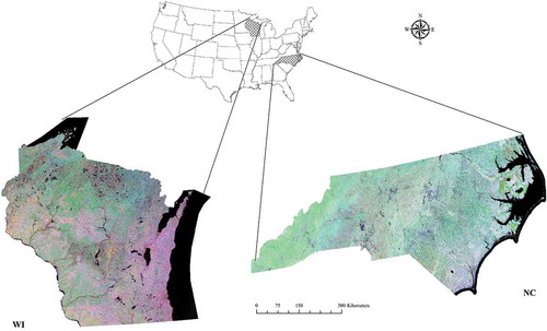
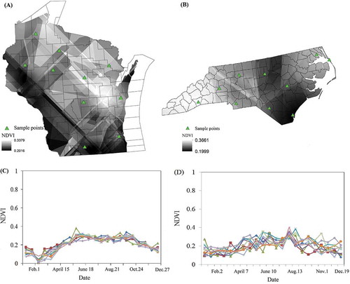
Figure 1. Study area: state of Wisconsin and North Carolina, USA. For full color versions of the figures in this article, please see the online version.

Endmember variability can be generally categorized as intra-class variability and inter-class variability (Zhang et al. 2006). The first one refers to the relative spectral differences within a specific endmember class, and the later one is associated with spectral variations among different classes. To overcome endmember variability, several studies have been conducted in the past decades through reducing intra-class variability or enhancing inter-class variability (Somers et al. 2011). Somers et al. (2011) first reviewed and compared all the proposed techniques for addressing the issue of endmember variability; they pointed out that the first attempt should be associated with the selection of appropriate spectral features for unmixng analysis. In particular, Asner and Lobell (2000) developed an autoSWIR approach to enhance between-class spectral variations through selecting the partial shortwave infrared (SWIR) spectral region. Moreover, statistical approaches, such as principal component analysis (PCA) (Johnson et al. 1993; Miao et al. 2006), discrete cosine transform (DCT) (Li 2004), and residual analysis (Ball, Bruce, and Younan 2007; Miao et al. 2006), have been proposed to select the best wavebands for spectral unmixing. Furthermore, Somers et al. (2010) developed a stable zone unmixing technique to select the bands with the lowest intra-class variation according to the instability index. Other techniques include spectral weighting, spectral transformation, and spectral transfer model. Chang and Ji (2006) proposed a weighted spectral mixture analysis (WSMA) to reduce endmember variability, with which higher weights were assigned to bands with relative low endmember variability. Further, Somers et al. (2009) developed a two-step weighting SMA through considering the variations of the reflected energy associated with each band. In addition to the spectral weighting techniques, spectral transformation has also been developed for mitigating within-class endmember variability. Wu (2004) developed normalized spectral mixture analysis to minimize the within-class endmember variability by normalizing the original spectra. This method was subsequently employed in geological applications (Zhang, Rivard, and Sanchez-Azofeifa 2005). In addition, Zhang, Rivard, and Sanchez-Azofeifa (2004) developed a derivative spectral unmixing (DSU) to address the variability issue through inputting the second-derivative endmember spectra in SMA. Although DSU is effective in solving the endmember variability issue, it also enhances high frequency noise. Thus, continuous wavelets techniques, and discrete wavelet and other wavelet analysis techniques, have been developed (Li 2004). With the wavelet analysis, transformed spectral features, instead of original reflectance features, have been employed in SMA (Li 2004; Rivard et al. 2008). Further, soil modeling mixture analysis was proposed to decrease within-class moisture differences for soil (Lobell et al. 2002; Somers et al. 2009).

In addition to the aforementioned techniques for addressing endmember variability, the other approach is the multiple endmember spectral mixture analysis (MESMA) method (Roberts et al. 1998), which considers all possible endmember combinations, and selects the best endmember set for each pixel. In MESMA, multiple endmembers were collected and saved in a spectra library, and numerous SMA models were constructed and tested with different combinations of types, numbers, and spectra of endmember classes for each individual pixel, and the best fit combination set was selected. Generally, the lowest root mean square error (RMSE) was used as the selection criterion. In addition, other selection techniques have also been developed, including count-based (Roberts et al. 2003), endmember average RMSE (EAR) (Dennison and Roberts 2003), minimum average spectral angle (Dennison, Halligan, and Roberts 2004), and iterative endmember selection (IES) (Schaaf et al. 2011). In addition to MESMA, the endmember bundles approach proposed by Bateson and Curtiss (1996) is the other trial-and-error technique for mitigating endmember variability. Specifically, instead of using only one endmember, a bundle of endmembers are collected and employed to construct endmember sets, and the minimum, mean, and maximum fractions for each land cover type are then extracted.

Although those proposed approaches have proven valuable in addressing endmember variability, there are still some challenging problems. In particular, most approaches still apply a set of fixed endmembers to extract image-wide land cover fractions. In fact, due to local variations of environmental and socioeconomic factors (e.g. topography, climate, economic development, population density, etc.), endmembers can be typically varied from location to location, and the selected endmembers may not be adequate to represent the complex conditions of a geographic area, which in turn results in erroneous estimates. While MESMA has addressed the endmember variability issue through including a variety of endmember sets, it is a pixel-based approach without considering geographic knowledge. Recently, Deng and Wu (2013) developed a spatial adaptive SMA (SASMA), with which local endmembers for a target pixel were selected within a moving window, and an inverse distance weighting (IDW) approach was applied to derive the endmembers for the target pixels. Spatial adaptive SMA, however, is a mathematical approach with empirically determined neighborhood size and distance-weighting functions (Li and Wu 2015).

Instead of employing single-date reflectance imagery, a temporal mixture analysis (TMA) was proposed by Knight and Voth (2011) using multiple-temporal NDVI (normalized difference vegetation index) data. The results show that the 2-year NDVI temporal profiles have achieved a satisfactory performance for estimating urban imperviousness. Further, Yang et al. (2012) applied TMA in Japan and demonstrated the ability of NDVI temporal profiles in estimating urban imperviousness at the national scale. Recently, Li and Wu (2014) proposed a phenology-based TMA (PTMA) and a phenology based multiple endmember temporal mixture analysis (PMETMA) with the highlight of the importance of phenological information derived from NDVI temporal profiles, and they found that with the extracted phenological information, one land cover type can be easily distinguished from another, and the issue of inter-class variability (such as the mixture of bare soil and impervious surface) can be effectively addressed. Furthermore, Li and Wu (2015) also successfully addressed the issue of endmember class selections through incorporating land use/land cover spatial information into TMA.

Although all proposed approaches have proven helpful for improving estimation accuracy, the issue of endmember variability has not been fully addressed. Therefore, in this study, we developed a geostatistical approach to approximate the “representative” endmembers for each individual pixel. In particular, we proposed to apply an ordinary kriging analysis method to interpolate the endmembers for each pixel. Ordinary kriging is a geostatistical approach and considered as a non-biased interpolation technique, as it can interpolate the value of a function at a given point by computing a weighted average of the known values of the function in the neighborhood of the point. It derives a best linear unbiased estimator based on assumptions on covariance and make use of the Gauss–Markov theorem to prove the independence of the estimate and error, and finally generate reasonable results. Ordinary kriging has been widely applied in soil mapping, population estimation, climatology, etc. (Cressie 1993; Vauclin et al. 1983; Wu and Murray 2005). This geostatistical temporal mixture analysis (GTMA) method can be divided into three steps: (1) identifying potential endmember candidates over the entire image using image endmember extraction and sampling, (2) calculating endmembers for each individual pixel using an ordinary kriging technique, and (3) estimating the endmember class fractions through spectral unmixing.

The rest of the article is structured as follows. Section 2 describes the selected study area and data source. Section 3 introduces the proposed GTMA approach, including endmember extraction and sampling, per-pixel endmember estimation using ordinary kriging, and fractional land cover estimation using fully constrained linear TMA. The estimation results of the proposed GTMA and comparative analyses with PTMA and PMETMA are reported in Section 4. Finally, discussion and conclusions are provided in Sections 5 and 6, respectively.

2. Study area and data

In order to test and verify the proposed approach, two research areas, states of Wisconsin (WI) and North Carolina (NC), were selected for this research (see Figure 1). Wisconsin is situated in the mid-western region of the United States with a geographic area of approximately 170,000 km² and the North Carolina state is located in the southeastern United States with an area of 139,390 km². These two states have experienced rapid urbanization during the past decades. According to the 2010 US census, the populations in Wisconsin and North Carolina were about 5.7 million and 9.5 million, and with increments of approximately 16% and 44%, respectively, from 1990 to 2010, and this trend was predicted to continue in the next decades (US Census Bureau 2014). Wisconsin and North Carolina are covered by a wide variety of land use/land cover types. Specifically, in Wisconsin, forest lands, including evergreen forest and deciduous forest, can be found in the northern part. Large patches of agricultural lands and pastures can be found in the southwest and northwest parts, respectively. Comparatively, urban areas, including Madison, Milwaukee, and Green Bay, are majorly distributed in the southeast part of the state. In North Carolina, agricultural lands and pastures can be found in the western and central parts, respectively; forests are mainly located in the central and eastern parts. Urban land uses, including a number of large cities, including Charlotte, Raleigh, Greensboro, and Durham, are majorly distributed in the central part of the state. As the major component of urbanized areas, impervious surfaces are composed of various man-made materials, such as asphalts for drive way, sidewalks and parking lots, concrete and cement for building rooftops, and tiles for residential house rooftops.

In order to map subpixel impervious surface fractions in Wisconsin and North Carolina through the proposed GTMA, 44 (22 for each study area) MODIS (moderate-resolution imaging spectroradiometer) NDVI images (1 band, product of MOD13Q1) acquired in 2006 were employed (two images per month, except the one in late November for Wisconsin and one in late August for North Carolina as heavy cloud covered). All images were collected from the United States Geological Survey (USGS) website (www.usgs.gov) with a 0.5-pixel positional accuracy and a spatial resolution of 250 meters. In addition to MODIS NDVI data, we also collected the National Land Cover Data (NLCD) 2006 Percent Developed Imperviousness data from the Multi-Resolution Land Characteristics Consortium (MRLC) website (http://www.mrlc.gov/nlcd06_data.php) for accuracy assessment. National Land Cover Data, generated by USGS, is the national land cover dataset that covers the entire United States. The data were produced based on Landsat TM/ETM+ imagery at a spatial resolution of 30 meters, and updated for every 5–10 years. For NLCD, the Anderson classification scheme was employed to classify the image into 10 major classes (see Table 1), and in this study, five land covers, including agriculture, deciduous forest, evergreen forest, pasture, and impervious surface were considered. Barren land and grassland were ignored due to their small areal coverages and the coarse resolution (250 m) of our remote sensing imagery. Further, water and wetlands were masked out before spectral unmixing to mitigate spectral confusion.

Table 1. Land covers types in the study areas.

Land cover type	Description
Urban	Areas with constructed materials and high number of impervious surfaces
Deciduous forest	Forest with trees losing the foliage seasonally
Evergreen forest	Forest with trees keeping leaves in all seasons
Pasture	Vegetation planted for livestock grazing
Grassland	Vegetation covered mainly by gramanoid or herbaceous, not subject to any intensive management
Agriculture	Areas for annual crops production
Barren land	Areas of glacial debris, sand, mines, bedrock, slides, desert pavement
Water	Areas of river, lake, reservoirs, streams
Wetland	Areas of forest or shrubland vegetation saturated with or covered with water

3. Methodology

To implement the proposed GTMA approach, three major steps were carried out, including endmember candidate extraction and sampling, spatially varying per-pixel endmember extraction using kriging, and fully constrained linear TMA. The details of these three steps are described as follows.

3.1. Endmember candidate extraction and sampling

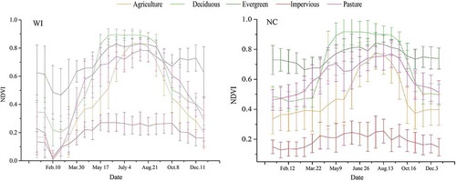
Endmember selection is the first and the most important step for successful spectral unmixing. Typically, PCA or minimum noise fraction (MNF) transformation is employed to guide the selection of endmembers. Due to the ability of ordering components on the basis of signal-to-noise ratios, MNF was applied in this study to remove noise and guide IES. In this study, several feature spaces were generated using the first several MNF components, and finally we found that all expected endmembers could be identified from scatterplots of the first three MNF components (see Figure 2). With the two-dimensional scatterplots generated using the first three MNF components, the vertices of these plots were selected as endmembers after verification with ground observations. These endmembers include agriculture, impervious surface, deciduous forest, evergreen forest, and pasture. Based on the pure spectra sets of endmembers chosen from the two-dimensional scatterplot, a stratified random sampling was applied for each class to collect endmembers for each class, and 200 endmember samples were selected for agriculture, deciduous forest, evergreen forest, and pasture, and 50 samples were chosen for impervious surfaces (as limited quantity of “pure” impervious surfaces exist) (see Figure 3). In order to show the spatial variation of the collected endmember samples, the NDVI temporal profiles of endmembers (calculated by averaging all samples of each endmember) including the first standard deviation were quantified and shown in Figure 4.

Figure 2. Two-dimensional scatterplot generated from MNF components.

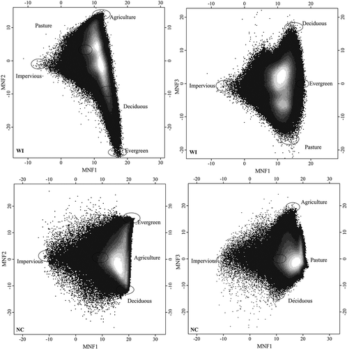
Figure 3. Spatial distribution of endmember class samples.

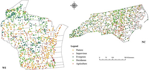
Figure 4. NDVI temporal profiles of selected endmember classes (including the first standard deviation).

3.2 Per-pixel endmember estimation using ordinary kriging

In order to apply ordinary kriging method to estimate the endmember for each class at per image pixel, a second moment stationary hypothesis (the correlation of two variables only associated with the spatial distance between them, and is not related to their location) test was conducted. The test results show that no significant variation can be detected and ordinary kriging analysis can be applied in further study. As the temporal profiles of each class include 22 NDVI bands in the stacked MODIS image, the ordinary kriging analysis needs to be implemented 22 times, each of which is to estimate the NDVI value for a particular band. The ordinary kriging was implemented with three major steps: (1) estimating the experimental variogram of an NDVI value of a specific band for a particular endmember class using collected samples, (2) fitting the estimated experimental variogram into a mathematical model, and (3) interpolating the NDVI value of the specific band for the endmember at each pixel. In this study, we identified five endmember classes (e.g. agriculture, impervious surface, deciduous forest, evergreen forest, and pasture) and each of them has 22-band NDVI temporal profiles. Therefore, this ordinary kriging process needs to be replicated for 110 times to derive the per-pixel endmembers for all endmember classes.

The details of this ordinary kriging process for estimating NDVI value for band b (1 ≤ b ≤ 22) of endmember class i are shown as follows. The first step is to estimate the experimental variogram using Equation (1):

(1)

where is the experimental variogram with a lag of d, NDVI_i,b,j and NDVI_i,b,k are the NDVI values of endmember samples j and k, respectively, and d_jk is the distance between samples j and k. In this study, the variogram was derived by using the mean value of all directions. With the knowledge of the spatial structure extracted from the experimental variogram, several theoretical mathematical models including circular, spherical, exponential, Gaussian, and linear models were applied to fit the experimental variogram, and the one with the highest R² was selected as the best-fit model. Following the guidance provided by Curran and Atkinson (1998) and McBratney and Webster (1986), a weighted least square fitting method was applied to derive the mathematical function of γ(d). With an appropriate mathematical expression of γ(d), kriging attempts to minimize the squares of the difference between the estimated and the reference NDVI values, expressed in Equation (2).

(2)

where is the estimated value of NDVI of band b of endmember class i at pixel s, NDVI_i,b,s and NDVI_i,b,j are the NDVI values for band b of endmember i at pixels s and j, respectively, and w_j and w_k are the weights of pixels j and k, respectively. To solve this optimization problem, a Lagrangian relaxation method was applied to derive the weights, as well as the NDVI value for pixel s. In this study, the experimental variograms and fitted mathematic model were calculated using GS+7.0, and ArcGIS10 was employed subsequently to implement the ordinary kriging for deriving the per-pixel endmember.

3.3 Fully constrained linear temporal mixture analysis

With the identified endmember classes and the corresponding endmembers derived from the ordinary kriging, a fully constrained linear TMA was conducted. The formulation of the TMA and the associated constraints are listed as follows:

(3)

where NDVI_b is the NDVI value for each band b, N is the total number of endmember classes (5), f_i is the fraction of endmember class i, NDVI_i,b is the NDVI value for band b of endmember i, and e_b is the residual. The TMA was carried out based on the assumption that the NDVI temporal profile of a mixed pixel (NDVI_b) is a linear combination of the estimated NDVI temporal profiles of all quantified endmember classes (NDVI_i,b), and the areal abundances (f_i) of all identified endmember classes can be extracted through implementing an inverse least squares deconvolution model. In order to present the physical meanings of the TMA results, the sum-to-one and non-negativity constraints were applied.

In order to assess the model fitness, the e_b and RMS error were applied. RMS error is typically used to measure the differences (also called residual) between predicted and observed values. It can be expressed as follows:

(4)

where B is the number of bands (22) of the MODIS NDVI image.

3.4 Comparative analysis and accuracy assessment

For comparative purposes, PTMA and PMETMA have also been implemented in this study. With PTMA, instead of using the localized endmembers derived from kriging analysis, a mean endmember set was calculated through averaging the collected endmembers, and this mean endmember set was subsequently applied for the whole image to estimate impervious surface fractions using the fully constrained linear TMA. Different from PTMA, PMETMA allows the use of a variety of endmember set combinations, and selects the one with the best model fit. For details of the PTMA and PMETMA models, readers can refer to Li and Wu (2014).

To assess the performance of the proposed GTMA, as well as those of PTMA and PMETMA, the NLCD 2006 Percent Developed Imperviousness data from USGS were applied in this study as the ground truth data, and a pixel-by-pixel comparison was conducted. Two widely used accuracy assessment metrics, systematic error (SE, Equation 5) and mean absolute error (MAE, Equation 6), were calculated to evaluate the performance of these three models. Specifically, SE quantifies the systematic bias (overestimation or underestimation), while MAE measures the overall accuracy.

(5)

(6)

where is the estimated impervious surface fraction for pixel j, f_j is the referenced impervious surface fraction value collected from NLCD 2006 impervious surface fractions for pixel j, and N is the total number of pixels.

4. Results

4.1 Spatially varying endmember estimation using ordinary kriging

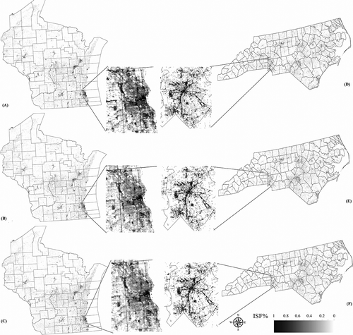
For estimating spatially varying per-pixel endmember for each endmember class, the ordinary kriging method was applied. Through analyzing the spatial variation structure of sampled endmembers for each class, we found that there is no significant anisotropy, and the variograms can be considered as isotropic. Results of experimental variograms and fitted exponential models of early August NDVI image (NDVI band 14), as an example, are illustrated in Figure 5. This result proves the existence of endmember variability, as well as the spatial autocorrelation of these endmembers. That is, the endmember of a pixel is likely to be similar to that of its neighboring pixels, and significantly different from those of pixels farther away. Moreover, the generally satisfactory R² values of these fit models indicate that it is appropriate to perform further interpolation analysis. In particular, the models for agriculture and pasture are with the highest R² (approximately 0.8), followed by evergreen with R² of 0.647 (WI) and 0.781 (NC), and the models of deciduous forest and impervious surfaces were also with R² of over 0.5. With the experimental variograms and fitted mathematical models, the endmember of each land cover type, e.g. agriculture, deciduous forest, evergreen forest, impervious surface, and pasture, was interpolated for each image pixel. Taking impervious surfaces as examples, Figure 6 indicates that the estimated endmember is with significant spatial variations. For example, a relatively high NDVI values (e.g. 0.34) in early August were found in the northern part of Wisconsin, and a rather low NDVI values (e.g. 0.20) were discerned in the southern portion. For North Carolina, a relatively high NDVI values (e.g. 0.36) in August can be found in the central part and a rather low NDVI values (e.g. 0.19) were distributed in the eastern part. In order to further illustrate the spatial variability of endmembers derived from the ordinary kriging, 10 samples were randomly selected in the study area, and the corresponding endmembers for impervious surfaces in Wisconsin and North Carolina are shown in Figure 6C and 6D. These results further prove the existence of spatial variations of endmembers, and endmember variability should be carefully examined before spectral unmixing. Artifacts of the impervious surface endmember distribution, however, do exist in Figure 6. In particular, it appears that low NDVI values are found in or around urban areas, and significantly higher NDVI values exist in rural areas (see Figure 6). This may be due to the lack of impervious surface endmember samples, as well as their uneven spatial distributions. Further improvements may include the adoption of a more quantitative approach for selecting a larger number and evenly distributed endmembers. This, however, might be difficult to achieve due to the scarcity of potential impervious surface endmember candidates.

Figure 5. Variograms of pure spectra of (A) agriculture, (B) deciduous forest, (C) evergreen forest, (D) impervious surface, and (E) pasture (take early August as an example).

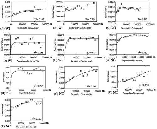
Figure 6. Interpolated impervious surface spectra using ordinary kriging for (A) WI and (B) NC, and sampled NDVI temporal profile for (C) WI and (D) NC (take early August as an example; colored lines are impervious surfaces temporal profiles from 10 sampling locations).

4.2 Fully constrained linear temporal mixture analysis

With the identified endmember classes and spatially varying per-pixel endmembers, we implemented the fully constrained linear TMA to extract the fractional land covers for each endmember class. Results (see Figure 7) illustrate that the spatial pattern of the modeled impervious surfaces corresponds well with our local knowledge of the study areas. In particular, high impervious surface fractions (ISF: 70–100%) are mainly located in the downtown area of urbanized areas such as Madison city (the state capital of Wisconsin) and Milwaukee city (the largest city of Wisconsin), and Charlotte (the largest city of North Carolina). Further, medium impervious surface fractions (ISF: 30–70%) are majorly distributed in the suburban areas such as Mequon, Grafton, and Oak Creek in Wisconsin and Concord, Gastonia in North Carolina, which can be commonly categorized as residential areas. In addition, low impervious surface fractions (ISF: 0–30%) can be easily found in the northern and western parts of Wisconsin and northern and eastern parts of North Carolina, which are majorly covered by vegetation. In addition to the visual examination, a quantitative analysis was also conducted for the whole study area, developed areas (ISF ≥ 30%), and less-developed areas (<30%). The 30% of ISA threshold is selected based on the definition of developed lands of the NLCD (http://www.epa.gov/mrlc/definitions.html). Results (see Table 2) indicate that the proposed GTMA has achieved a promising accuracy in modeling the ISF for both study areas. Specifically, in Wisconsin, the overall study area was with an SE of 2.98% and an MAE of 3.83%, and in North Carolina, the whole study area was with an SE of 3.98% and an MAE of 5.61%. Detailed analysis indicates that GTMA performs better in less-developed areas (MAE = 3.71% (WI), 5.39% (NC)) than in developed areas (MAE = 9.36% (WI), 7.19% (NC)), and a slight overestimation (WI: 3.07%; NC: 3.98%) for less-developed areas and slight underestimation (WI: −1.49%; NC: −3.11%) for developed areas have been detected.

Table 2. Accuracy assessment of impervious surfaces with GTMA, PTMA, and PMETMA.

			SE (%)	MAE (%)
Wisconsin	GTMA	Overall	2.98	3.83
		Developed	−1.49	9.36
		Less developed	3.07	3.71
	PTMA	Overall	3.25	4.03
		Developed	−8.17	12.15
		Less developed	3.43	3.9
	PMETMA	Overall	2.13	3.36
		Developed	−7.46	12.16
		Less developed	2.32	3.23
North Carolina	GTMA	Overall	3.98	5.61
		Developed	−3.11	7.19
		Less developed	4.73	5.39
	PTMA	Overall	5.45	6.07
		Developed	−6.58	10.63
		Less developed	5.51	5.8
	PMETMA	Overall	3.44	5.45
		Developed	−5.96	11.62
		Less developed	3.65	5.37

Figure 7. Estimated impervious surface fraction maps from GTMA (A: WI, D: NC), PTMA (B: WI, E: NC), and PMETMA (C: WI, F: NC).

4.3 Comparative analysis

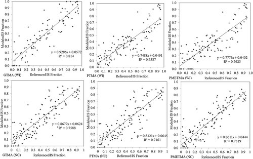
For comparison, PTMA and PMETMA were also implemented; the RMS for every image pixel was calculated to show the model performance (see Figure 8), and the impervious surfaces estimation results are illustrated in Figure 7 and Table 2. Figure 8 shows that the RMS of GTMA model is generally better than that of PTMA and PMETMA, and the average RMS values of GTMA are 0.0324 vs. 0.0385 (PTMA) and 0.0381 (PMETMA) in Wisconsin and 0.0417 vs. 0.0433 (PTMA) and 0.0431 (PMETMA) in North Carolina. The estimation results (see Figure 7) indicate that impervious surface fraction maps generated from GTMA, PTMA, and PMETMA are with similar spatial distribution patterns. In particular, higher impervious surface fraction values can be found in the southeast Wisconsin (e.g. Milwaukee city) and central North Carolina (e.g. Charlotte city), and significantly lower impervious surface fraction values are located in the western and northern Wisconsin and western and eastern North Carolina covered by wetlands, agriculture, and forest. Although with similar spatial patterns, one noticeable difference can be found in urban areas. That is, with PTMA and PMETMA, impervious surface fraction estimates in urban areas are much lower than those estimated with GTMA. In order to illustrate the improvement in developed areas, Milwaukee and Charlotte, two largest cities in Wisconsin and North Carolina were also selected, and comparative maps are shown in Figure 7. It indicates that obvious underestimation can be detected with PTMA and PMETMA, and this problem has been effectively addressed with GTMA. Further quantitative analysis confirms these visual observations. For the entire study area, as well as less-developed areas, the performances of PTMA and PMETMA are comparable to that of GTMA. That is, these three models are with similar SE and MAE values. In urban areas, however, the performances of PTMA and PMETMA are significantly worse than that of GTMA. For instance, in urban areas, the SE values of PTMA and PMETMA are (WI: −8.17%; NC: −6.58%) and (WI: −7.46%; NC: −5.96%) respectively, significantly higher than that of GTMA (WI: −1.49%; NC: −3.11%). Moreover, in urban areas, the MAE values of PTMA and PMETMA are 12.15% (WI) and 10.63% (NC), and 12.16% (WI) and 11.62% (NC) respectively, much higher than those of GTMA (WI: 9.36%; NC: 7.19%). Moreover, in order to illustrate the relationship between the modeled and referenced impervious surface fractions, a scatterplot was also created through stratified randomly selected samples (see Figure 9). Figure 9 shows that with the proposed GTMA, the underestimation in the developed areas has been highly addressed, and generally, the proposed GTMA has achieved a better performance with a higher R². In summary, when compared to PTMA and PMETMA, the proposed GTMA has achieved a comparable performance for the whole study area and less-developed areas, and a much better performance for developed areas.

Figure 8. RMS of GTMA, PTMA, and PMETMA.

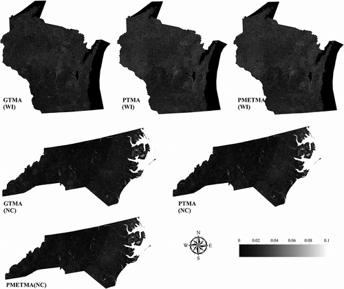
Figure 9. Accuracy assessment of the impervious surfaces estimation by the GTMA, PTMA, and PMETMA.

5. Discussion

5.1 Estimating spatially varying per-pixel endmembers using geostatistical techniques

Endmember selection has been widely considered as a key step of spectra unmixing, and exerts significant impact on the estimation accuracy of fractional land covers. Specifically, as environmental factors vary spatially, endmember spectra tend to be different across space. However, derived endmember spectra are often considered identical and applied to all the pixels in a remote sensing image. While MESMA accommodates endmember variability through employing a variety of endmember sets, it only employs pixel-based spectral information, without considering spatial knowledge. Recently, the SASMA proposed by Deng and Wu (2013) attempted to address endmember variability through deriving endmembers for a particular pixel through applying an IDW approach using all endmember candidates in a moving window. This approach, however, only employs the distance for generating weights, and the statistical meanings of the spatial variations of endmembers have been neglected. As a consequence, inappropriate endmembers may be selected and applied in SMA and result in erroneous estimations. The proposed GTMA is able to address the aforementioned issues. In particular, a spatially varying per-pixel endmember was calculated for each image pixel using a rigorous geostatistical technique, ordinary kriging interpolation technique.

5.2. Endmember variability in developed and less-developed areas

Compared with the results we derived from PTMA and PMETMA (Li and Wu 2014), the performance of GTMA is comparable in the whole study area and less-developed areas. The improvements in developed areas (see Figure 7), however, are much more significant (WI: SE of −1.49% vs. −8.17% and −7.46%, and MAE of 9.36% vs. 12.15% and 12.16%; NC: SE of −3.11% vs. −6.58% and −5.96%, and MAE of 7.19% vs. 10.63% and 11.62%) when compared to less-developed areas. These results might indicate that endmember variability plays an even more important role in developed areas than in less-developed areas. This may be due to the complexity and heterogeneity of urban landscapes. That is, unlike less-developed areas with relatively homogenous land cover types and corresponding spectral signatures, developed areas are covered by heterogeneous and anthropogenic materials with different physical and chemical compositions. For instance, impervious surfaces may be comprised by several different materials for different purposes, such as asphalts for drive way, sidewalks, and parking lot, concrete and cement for building rooftop, and tiles for residential house rooftops. In addition, the same building materials with different ages may also show quite different spectral responses. As a result, endmember variability may play a more essential role in developed areas when compared to less-developed areas. The advantages of the proposed GTMA approach, therefore, are to better approximate the spatially varying per-pixel endmembers, especially for developed areas with heterogeneous and anthropogenic materials.

6. Conclusions and future research directions

This study developed a GTMA approach to address the endmember variability issue for estimating regional impervious surface distributions using time-series MODIS NDVI imagery acquired in Wisconsin and North Carolina, United States. In particular, an ordinary kriging interpolation technique was employed to extract spatially varying pixel-specific endmembers. Consequently, a fully constrained linear TMA with spatially varying endmember was developed to quantify impervious surface distributions.

Analysis of results suggests several conclusions. First, the proposed GTMA has achieved a satisfactory performance for examining the fractions of impervious surfaces in the entire study area of Wisconsin with an SE of 2.98% and MAE of 3.83%, and in the state of North Carolina with an SE of 4.73% and MAE of 5.39%. Detailed analysis indicates that a better performance has been achieved in less-developed areas than in developed areas, and slight underestimation and slight overestimation have been detected in developed areas and less-developed areas, respectively. Second, for a comparative purpose, PTMA and PMETMA have been implemented, and the comparative analysis results indicate that the proposed GTMA has achieved a comparable performance with PTMA and PMETMA in the overall area and less-developed area. However, a significant improvement has been found in developed areas of Wisconsin and North Carolina with the SE of −1.49% (vs. −8.17% and −7.46%) and −3.11% (vs. −6.58% and −5.96%), MAE of 9.36% (vs. 12.15% and 12.16%) and 7.19% (vs. 10.63% and 11.62%) respectively.

Although the proposed GTMA has achieved a promising accuracy for estimating impervious surface fractions through addressing endmember variability, endmember class variability has not been fully considered in this study. In fact, the selection of endmember classes is the foundation of endmember extraction, and it may play a very important role in successfully spectral unmixing. Therefore, one future research could be considering both endmember class variability and endmember variability through constructing an integrated TMA model to improve the estimation accuracy. In addition, in this study, only local spatial information has been incorporated in spectral unmixing analysis, and regional spatial information has been more or less neglected. However, such information may also be helpful in addressing the endmember variability issue. Therefore, another future research direction could be incorporating both regional and local spatial information into TMA.

Disclosure statement

No potential conflict of interest was reported by the authors.

Additional information

Funding

This work was supported by the National Natural Science Foundation of China [41030743] and Research and Creative Activities Award of the University of Wisconsin – Milwaukee.

References

- Asner, G. P., and D. B. Lobell. 2000. “A Biogeophysical Approach for Automated SWIR Unmixing of Soils and Vegetation.” Remote Sensing of Environment 74: 99–112. doi:10.1016/S0034-4257(00)00126-7.
- Ball, J. E., L. M. Bruce, and N. H. Younan. 2007. “Hyperspectral Pixel Unmixing via Spectral Band Selection and DC-Insensitive Singular Value Decomposition.” IEEE Transactions on Geoscience and Remote Sensing Letters 4: 382–386. doi:10.1109/LGRS.2007.895686.
- Bateson, A., and B. Curtiss. 1996. “A Method for Manual Endmember Selection and Spectral Unmixing.” Remote Sensing of Environment 55: 229–243. doi:10.1016/S0034-4257(95)00177-8.
- Bateson, C. A., G. P. Asner, and C. A. Wessman. 2000. “Endmember Bundles: A New Approach to Incorporating Endmember Variability into Spectral Mixture Analysis.” IEEE Transactions on Geoscience and Remote Sensing 38: 1083–1094. doi:10.1109/36.841987.
- Bedini, E. 2009. “Mapping Lithology of the Sarfartoq Carbonatite Complex, Southern West Greenland, Using Hymap Imaging Spectrometer Data.” Remote Sensing of Environment 113: 1208–1219. doi:10.1016/j.rse.2009.02.007.
- Bhatti, S., and N. Tripathi. 2014. “Built-Up Area Extraction Using Landsat 8 OLI Imagery.” GIScience & Remote Sensing 51: 445–467. doi:10.1080/15481603.2014.939539.
- Chang, C.-I., and B. H. Ji. 2006. “Weighted Abundance-Constrained Linear Spectral Mixture Analysis.” IEEE Transactions on Geoscience and Remote Sensing 44: 378–388. doi:10.1109/TGRS.2005.861408.
- Cressie, N. 1993. Statistics for Spatial Data. Revised ed. New York: Wiley.
- Cunningham, S., J. Rogan, D. Martin, V. Delauer, S. McCauley, and A. Shatz. 2015. “Mapping Land Development through Periods of Economic Bubble and Bust in Massachusetts Using Landsat Time Series Data.” GIScience & Remote Sensing 52: 397–415. doi:10.1080/15481603.2015.1045277.
- Curran, P. J., and P. M. Atkinson. 1998. “Geostatistics and Remote Sensing.” Progress in Physical Geography 22: 61–78. doi:10.1177/030913339802200103.
- Deng, C., and C. Wu. 2013. “A Spatially Adaptive Spectral Mixture Analysis for Mapping Subpixel Urban Impervious Surface Distribution.” Remote Sensing of Environment 133: 62–70. doi:10.1016/j.rse.2013.02.005.
- Dennison, P. E., K. Q. Halligan, and D. A. Roberts. 2004. “A Comparison of Error Metrics and Constraints for Multiple Endmember Spectral Mixture Analysis and Spectral Angle Mapper.” Remote Sensing of Environment 93: 359–367. doi:10.1016/j.rse.2004.07.013.
- Dennison, P. E., and D. A. Roberts. 2003. “Endmember Selection for Multiple Endmember Spectral Mixture Analysis Using Endmember Average RMSE.” Remote Sensing of Environment 87: 123–135. doi:10.1016/S0034-4257(03)00135-4.
- Eckmann, T. C., C. J. Still, D. A. Roberts, and J. C. Michaelsen. 2010. “Variations in Subpixel Fire Properties with Season and Land Cover in Southern Africa.” Earth Interactions 14: 1–29. doi:10.1175/2010EI328.1.
- Elmore, A. J., J. F. Mustard, S. J. Manning, and D. B. Lobell. 2000. “Quantifying Vegetation Change in Semiarid Environments: Precision and Accuracy of Spectral Mixture Analysis and the Normalized Difference Vegetation Index.” Remote Sensing of Environment 73: 87–102. doi:10.1016/S0034-4257(00)00100-0.
- Gilabert, M. A., F. J. Garcı́a-Haro, and J. Meliá. 2000. “A Mixture Modeling Approach to Estimate Vegetation Parameters for Heterogeneous Canopies in Remote Sensing.” Remote Sensing of Environment 72: 328–345. doi:10.1016/S0034-4257(99)00109-1.
- Herold, M., D. A. Roberts, M. E. Gardner, and P. E. Dennison. 2004. “Spectrometry for Urban Area Remote Sensing-Development and Analysis of a Spectral Library from 350 to 2400 Nm.” Remote Sensing of Environment 91: 304–319. doi:10.1016/j.rse.2004.02.013.
- Hestir, E. L., S. Khanna, M. E. Andrew, M. J. Santos, J. H. Viers, J. A. Greenberg, S. S. Rajapakse, and S. L. Ustin. 2008. “Identification of Invasive Vegetation Using Hyperspectral Remote Sensing in the California Delta Ecosystem.” Remote Sensing of Environment 112: 4034–4047. doi:10.1016/j.rse.2008.01.022.
- Jia, G. J., I. C. Burke, A. F. H. Goetz, M. R. Kaufmann, and B. C. Kindel. 2006. “Assessing Spatial Patterns of Forest Fuel Using AVIRIS Data.” Remote Sensing of Environment 102: 318–327. doi:10.1016/j.rse.2006.02.025.
- Johnson, P. E., M. O. Smith, S. Taylorgeorge, and J. B. Adams. 1993. “A Semiempirical Method for Analysisi of the Reflectance Spectra of Binary Mineral Mixtures.” Journal of Geographical Research 88: 3557–3561. doi:10.1029/JB088iB04p03557.
- Keshava, N. 2003. “Survey of Spectral Unmixing Algorithms.” Lincoln Laboratory Journal 14: 55–78.
- Knight, J. F., and M. Voth. 2011. “Mapping Impervious Cover Using Multi-Temporal MODIS NDVI Data.” IEEE Journal of Selected Topics in Applied Earth Observations and Remote Sensing 4: 303–309. doi:10.1109/JSTARS.2010.2051535.
- Lelong, C. C. D., P. C. Pinet, and H. Poilvé. 1998. “Hyperspectral Imaging and Stress Mapping in Agriculture: A Case Study on Wheat in Beauce (France).” Remote Sensing of Environment 66: 179–191. doi:10.1016/S0034-4257(98)00049-2.
- Li, G., D. Lu, E. Moran, and S. Hetrick. 2013. “Mapping Impervious Surface Area in the Brazilian Amazon Using Landsat Imagery.” GIScience & Remote Sensing 50: 172–183. doi:10.1080/15481603.2013.780452.
- Li, J. 2004. “Wavelet-Based Feature Extraction for Improved Endmember Abundance Estimation in Linear Unmixing of Hyperspectral Signals.” IEEE Transactions on Geoscience and Remote Sensing 42: 644–649. doi:10.1109/TGRS.2003.822750.
- Li, W., and C. Wu. 2014. “Phenology-Based Temporal Mixture Analysis for Estimating Large-Scale Impervious Surface Distributions.” International Journal of Remote Sensing 35: 779–795. doi:10.1080/01431161.2013.873147.
- Li, W., and C. Wu. 2015. “Incorporating Land Use Land Cover Probability Information into Endmember Class Selections for Temporal Mixture Analysis.” ISPRS Journal of Photogrammetry and Remote Sensing 101: 163–173. doi:10.1016/j.isprsjprs.2014.12.007.
- Liu, J., J. R. Miller, D. Haboudane, E. Pattey, and K. Hochheim. 2008. “Crop Fraction Estimation from Casi Hyperspectral Data Using Linear Spectral Unmixing and Vegetation Indices.” Canadian Journal of Remote Sensing 34: S124–S138. doi:10.5589/m07-062.
- Lobell, D. B., G. P. Asner, B. E. Law, and R. N. Treuhaft. 2002. “View Angle Effects on Canopy Reflectance and Spectral Mixture Analysis of Coniferous Forests Using AVIRIS.” International Journal of Remote Sensing 23: 2247–2262. doi:10.1080/01431160110075613.
- McBratney, A. B., and R. Webster. 1986. “Choosing Functions for Semi-Variograms of Soil Properties and Fitting Them to Sampling Estimates.” Journal of Soil Science 37: 617–639. doi:10.1111/j.1365-2389.1986.tb00392.x.
- Miao, X., P. Gong, S. Swope, R. Pu, R. Carruthers, G. L. Anderson, J. S. Heaton, and C. R. Tracy. 2006. “Estimation of Yellow Starthistle Abundance through CASI-2 Hyperspectral Imagery Using Linear Spectral Mixture Models.” Remote Sensing of Environment 101: 329–341. doi:10.1016/j.rse.2006.01.006.
- Qiu, X., S. Wu, and X. Miao. 2014. “Incorporating Road and Parcel Data for Object-Based Classification of Detailed Urban Land Covers from NAIP Images.” GIScience & Remote Sensing 51: 498–520. doi:10.1080/15481603.2014.963982.
- Rhee, J., S. Park, and Z. Lu. 2014. “Relationship between Land Cover Patterns and Surface Temperature in Urban Areas.” GIScience & Remote Sensing 51: 521–536. doi:10.1080/15481603.2014.964455.
- Rivard, B., J. Feng, A. Gallie, and A. Sanchez-Azofeifa. 2008. “Continuous Wavelets for the Improved Use of Spectral Libraries and Hyperspectral Data.” Remote Sensing of Environment 112: 2850–2862. doi:10.1016/j.rse.2008.01.016.
- Roberts, D. A., P. E. Dennison, M. E. Gardner, Y. Hetzel, S. L. Ustin, and C. T. Lee. 2003. “Evaluation of the Potential of Hyperion for Fire Danger Assessment by Comparison to the Airborne Visible/Infrared Imaging Spectrometer.” IEEE Transactions on Geoscience and Remote Sensing 41: 1297–1310. doi:10.1109/TGRS.2003.812904.
- Roberts, D. A., M. Gardner, R. Church, S. Ustin, G. Scheer, and R. O. Green. 1998. “Mapping Chaparral in the Santa Monica Mountains Using Multiple Endmember Spectral Mixture Models.” Remote Sensing of Environment 65: 267–279. doi:10.1016/S0034-4257(98)00037-6.
- Rosa, D., and D. Wiesmann. 2013. “Land Cover and Impervious Surface Extraction Using Parametric and Non-Parametric Algorithms from the Open-Source Software R: An Application to Sustainable Urban Planning in Sicily.” GIScience & Remote Sensing 50: 231–250. doi:10.1080/15481603.2013.795307.
- Sabol, D. E., J. B. Adams, and M. O. Smith. 1992. “Quantitative Subpixel Spectral Detection of Targets in Multispectral Images.” Journal of Geophysical Research: Planets 97: 2659–2672. doi:10.1029/91JE03117.
- Schaaf, A., P. Dennison, G. Fryer, K. Roth, and D. Roberts. 2011. “Mapping Plant Functional Types at Multiple Spatial Resolutions Using Imaging Spectrometer Data.” GIScience & Remote Sensing 48: 324–344. doi:10.2747/1548-1603.48.3.324.
- Somers, B., G. P. Asner, L. Tits, and P. Coppin. 2011. “Endmember Variability in Spectral Mixture Analysis: A Review.” Remote Sensing of Environment 115: 1603–1616. doi:10.1016/j.rse.2011.03.003.
- Somers, B., S. Delalieux, J. Stuckens, W. W. Verstraeten, and P. Coppin. 2009. “A Weighted Linear Spectral Mixture Analysis Approach to Address Endmember Variability in Agricultural Production Systems.” International Journal of Remote Sensing 30: 139–147. doi:10.1080/01431160802304625.
- Somers, B., J. Verbesselt, E. M. Ampe, N. Sims, W. W. Verstraeten, and P. Coppin. 2010. “Spectral Mixture Analysis to Monitor Defoliation in Mixed-Aged Eucalyptus Globulus Labill Plantations in Southern Australia Using Landsat 5-TM and EO-1 Hyperion Data.” International Journal of Applied Earth Observation and Geoinformation 12: 270–277. doi:10.1016/j.jag.2010.03.005.
- Tompkins, S., J. F. Mustard, C. M. Pieters, and D. W. Forsyth. 1997. “Optimization of Endmembers for Spectral Mixture Analysis.” Remote Sensing of Environment 59: 472–489. doi:10.1016/S0034-4257(96)00122-8.
- US Census Bureau. 2014. “National Population Projections.” http://www.census.gov/population/projections/data/national/
- Vauclin, M., S. R. Vieira, G. Vachaud, and D. R. Nielsen. 1983. “The Use of Cokriging with Limited Field Soil Observations.” Soil Science Society of America Journal 47: 175–184. doi:10.2136/sssaj1983.03615995004700020001x.
- Wu, C. 2004. “Normalized Spectral Mixture Analysis for Monitoring Urban Composition Using ETM+ Imagery.” Remote Sensing of Environment 93: 480–492. doi:10.1016/j.rse.2004.08.003.
- Wu, C., and A. T. Murray. 2003. “Estimating Impervious Surface Distribution by Spectral Mixture Analysis.” Remote Sensing of Environment 84: 493–505. doi:10.1016/S0034-4257(02)00136-0.
- Wu, C., and A. T. Murray. 2005. “A Cokriging Method for Estimating Population Density in Urban Areas.” Computers, Environment and Urban Systems 29: 558–579. doi:10.1016/j.compenvurbsys.2005.01.006.
- Yang, F., B. Matsushita, T. Fukushima, and W. Yang. 2012. “Temporal Mixture Analysis for Estimating Impervious Surface Area from Multi-Temporal MODIS NDVI Data in Japan.” ISPRS Journal of Photogrammetry and Remote Sensing 72: 90–98. doi:10.1016/j.isprsjprs.2012.05.016.
- Zhang, J., B. Rivard, A. Sanchez-Azofeifa, and K. Castro-Esau. 2006. “Intra and Inter-Class Spectral Variability of Tropical Tree Species at La Selva, Costa Rica: Implications for Species Identification Using HYDICE Imagery.” Remote Sensing of Environment 105: 129–141. doi:10.1016/j.rse.2006.06.010.
- Zhang, J. K., B. Rivard, and A. Sanchez-Azofeifa. 2004. “Derivative Spectral Unmixing of Hyperspectral Data Applied to Mixtures of Lichen and Rock.” IEEE Transactions on Geoscience and Remote Sensing 42: 1934–1940. doi:10.1109/TGRS.2004.832239.
- Zhang, J. K., B. Rivard, and A. Sanchez-Azofeifa. 2005. “Spectral Unmixing of Normalized Reflectance Data for the Deconvolution of Lichen and Rock Mixtures.” Remote Sensing of Environment 95: 57–66. doi:10.1016/j.rse.2004.11.019.