An improved topographic correction model based on Minnaert

Abstract

The uneven distribution of solar radiation due to topographic relief can significantly change the correlation between reflectance and other features such as biomass in rugged terrain regions. In this article, we use the transfer theory to improve the Minnaert approach. After comparing topographic correction methods for Landsat 8 Operational Land Imager (OLI) and EO-1 Advanced Land Imager (ALI) imagery acquired from the mountainous region in Beijing, China, we used visual inspection, statistical analysis, and correlation analysis to evaluate the algorithms and performance of the proposed Minnaert-E approach. The results indicate that corrections based on non-Lambertian methods have better performance than those based on the Lambertian assumption. The correction performances can be ranked as the Minnaert-E, followed by the Minnaert and the SCS+C corrections, and, finally, the C-HuangWei correction, which performed the worst. We found that the Minnaert-E approach can effectively weaken the influence of terrain relief on pixels and restore the true reflectance of the pixels in the relief area. Further analysis indicates that the Minnaert-E has a better effect on image processing where the slope gradient is restricted to less than 10° or between 30° and 43°.

Keywords:

• topographic correction
• non-Lambertian reflection models
• sky isotropic scattering
• adjacent terrain reflection
• Landsat 8 OLI

1. Introduction

Topographic correction refers to the transformation of the radiation brightness values or reflectance of all pixels from a slanted plane to another reference plane (usually horizontal), to eliminate the effect caused by topographic relief (Gao et al. 2014). Topographic correction is an important step in the radiation correction of remote sensing imagery in mountainous areas, as well as a topic for quantitative remote sensing research (Li, Im, and Beier 2013).

Over the past 30 years, the negative effects of terrain relief on land use/land cover (LULC) data have been discussed in several studies (Gu and Gillespie 1998; Wu et al. 2008), and various topographic correction methods have been developed in response. Well-known statistical models, including the Teillet-regression correction method (Teillet, Guindon, and Goodenough 1982) and the b correction method (Vincini, Reeder, and Frazzi 2002), primarily exploit the correlation between image brightness values and the cosine of the angle of sun incidence. Civco (1989) proposed a normalized model, known as the “two classes” correction method, which comprises two stages of process. In the early 1980s, Teillet, Guindon, and Goodenough (1982) introduced the physical cosine model based on the assumption of single-band bidirectional reflectance parameters. They then improved this model and renamed it, now known as the C correction model (Gao and Zhang 2008). However, because of defects in the assumption of the Lambertian theory, the C correction method has since been improved many times to meet different requirements (Civco 1989; Huang, Zhang, and Li 2005; Chen 2006, 2006). Gu and Gillespie (1998) proposed the sun-canopy-sensor (SCS) model, which is based on the relationship between the sun radiation, the vegetation canopy, and the sensor. But the SCS model still had an overcorrection problem since it ignored sky isotropic scattering and the reflection from adjacent terrains. The phenomenon of overcorrection was never fully resolved until Soenen, Peddle, and Coburn (2005) introduced a parameter C based on the C correction concept and developed the SCS+C model. In the early 1980s, Smith, Lin, and Ranson (1980) introduced the Minnaert algorithm based on non-Lambertian reflectance models, which includes the empirical constant k to effectively weaken the degree of overcorrection. Subsequently, Reeder (2002) presented the Minnaert-SCS model by introducing the principles of the SCS algorithm to the model, thus simultaneously simplifying the required parameters. Hantson and Chuvieco (2011) compared different topographic correction results on multitemporal Landsat ETM+ data, and their statistical results showed that for a single image, the C correction and Minnaert models were more appropriate, while for long-term multitemporal data, the C correction model alone performed better. Shi, Yang, and Mu (2009) proposed a new topographic correction model by introducing the radiation-scaling factor, using the lookup table established by the Second Simulation of the Satellite Signal in the Solar Spectrum (6S) atmospheric correction model. Wen et al. (2008) introduced an optical remote sensing reflectance model, which was based on the directional reflection theory and the radiation transfer equation.

In this article, by considering sky isotropic scattering and reflection from the adjacent terrain, we further improve the Minnaert model performance of previous studies. The improvements are based on non-Lambertian reflection and radiation transmission theories, and we used Landsat 8 Operational Land Imager (OLI) and the EO-1 Advanced Land Imager (ALI) images as experiments. We performed visual inspection, and statistical and correlation analyses to evaluate the topographic corrections. In addition, we evaluated the improved Minneart-E approach by comparing our results with those from four commonly used correction methods: the cosine, the C-HuangWei, the SCS+C, and the Minnaert methods.

2. Material and methods

2.1. Commonly used topographic correction methods

Digital elevation model (DEM)-based models can be broadly classified into four categories, including empirical-statistical models (Teillet, Guindon, and Goodenough 1982; Vincini, Reeder, and Frazzi 2002), the normalized model (Civco 1989), the Lambertian reflectance model (Dymond and Shepherd 1999), and non-Lambertian reflectance models (Ekstrand 1996; Soenen, Peddle, and Coburn 2005; Richter, Kellenberger, and Kaufmann 2009). In some papers, the normalized model was also classified as an empirical method (Gao and Zhang 2009), which yielded the best results for training areas statistics in the Law and Nichol study (2004). Table 1 presents several commonly used Lambertian and non-Lambertian reflection methods.

Table 1. Topographic correction models used in this study.

	Topographic correction models	Expression	Presenter
1	Cosine		Teillet, Guindon, and Goodenough (1982)
2	C-HuangWei		Huang, Zhang, and Li (2005)
3	SCS+C		Soenen, Peddle, and Coburn (2005)
4	Minnaert		Smith, Lin, and Ranson (1980)

Where: L_m = radiance after correction; L = radiance before correction; L_min = minimum radiance before correction; θ_s = solar zenith angle; S = slope; i = solar incident angle; e = angle of incidence for the receiving sensor. In this article, the e value is equal to S due to the satellite angle of tilt; C = empirical constant; k = Minnaert constant.

2.2. Improvement of the Minnaert: Minnaert-E model

Previous authors have suggested that the Minnaert approach based on non-Lambertian assumptions performed better than other Lambertian-based topographic corrections, especially regarding the visual effect (Law and Nichol 2004). However, by ignoring sky isotropic scattering and the surrounding terrain reflectance, the correction results of the Minnaert method seemed less than satisfactory (Gao and Zhang 2008). In addition, the linearization of the parameter k (Wu et al. 2008) also ignored sky isotropic scattering and environmental reflection. In the visible spectrum, the above-mentioned scattering accounts for a larger proportion of the total incident irradiance, thus it would weaken the linear relationship between the cosine of the solar incident angle (also known as solar illumination) and the irradiance recorded by pixels.

In the remote sensing of mountainous areas, if the multiple reflections between the land surface and the atmosphere are ignored, the sum of the solar radiation received by the earth can be divided into three parts: direct solar radiation, sky (diffuse) scattering radiation, and terrain-reflected radiation. The total solar radiation that a pixel receives for a mountainous slope can be expressed as follows:

(1)

where Θ is the shadows cast, and for pixels in shadow, Θ is equal to 0, otherwise Θ is equal to 1; represents the direct solar radiation received by a pixel, is the sky isotropic scattering radiation the pixel receives, while is the terrain-reflected radiation. With the assumption that a certain range of atmosphere in the study area is composed of several sheets with uniform structure in the horizontal direction, the direct solar radiation exposure to the slope pixels can be defined as follows:

(2)

where stands for the ESUNI (solar irradiation at the top of the atmosphere) related to the wavelength (λ); τ is the atmospheric optical thickness (AOT); cos θ_s is the cosine value of the solar zenith angle; is the atmospheric transmissivity, and represents the direct solar radiation penetrating through the atmosphere, which can be computed by the 6S model. d_r is the Sun–Earth distance in astronomical units. Furthermore, if sky anisotropy scattering is disregarded, and we instead assume that the sky scattering is isotropic, then the sky scattering isotropic radiation in complex terrain regions can be expressed using the following equation:

(3)

where is the sky isotropic scattering irradiance without any topographic effects, which can also be calculated by the 6S model, and is the sky-view factor.

 +  is the summation of the sky (diffuse) scattering and terrain reflection, which has been so difficult to determine, due to the complex calculation process involved, that it has created barriers for those attempting to understand and discuss the theory behind it (Hay and McKay 1985). Dozier and Frew (1990) simplified the additional calculation process for the adjacent terrain reflection, thereby improving its efficiency. However, mean value has been used to calculate the reflectance of pixels in shadow, rather than the true reflectance. As a result, advances in correcting results for shady slopes have not been significant.

In order to further improve these calculations, based on the Lambertian assumption and the hypothesis from Gao and Zhang (2008), we assumed that r is the ratio of the sky scattering radiation received by the Earth () and the ESUNI, thus . Then Equation (3) can be expressed as follows:

(4)

Ignoring the multiple reflections between the Earth’s surface and the atmosphere, we can derive the terrain reflection from the radiation at the base of the atmosphere caused by terrain structure and surface reflectivity. Thus, the terrain reflection can be defined as follows:

(5)

where is the terrain configuration factor, is the reflectivity of the adjacent pixels, and is the reflectivity of adjacent terrain reflected radiation.

Dozier and Frew (1990) concluded that the relationship between the sky-view factor and terrain configuration factor could be approximately expressed as follows:

(6)

As the sky-view factor is approximately calculated through the analytical approach, here we directly use these authors’ conclusions in the following equation:

(7)

where S is the slope derived from the DEM, which matches with each pixel in the satellite image. Then, substituting Equations (2)–(7) into Equation (1), a new equation for describing the solar radiation received by the pixels of a mountainous slope may be expressed as follows:

(8)

If we then multiply each term on both sides of the equation by the equivalent reflectivity, Equation (8) is transformed into an expression of irradiance:

(9)

where stands for the apparent spectral radiance after sensor calibration, and represents the equivalent radiance near the Earth’s surface. Without sky scattering and surrounding terrain reflection, using the Minnaert approach, the satellite radiance can be calculated by the following formula:

(10)

where is the true radiance after topographic correction, is the radiance value before correction, and is the angle of incidence for the receiving sensor. The factor is the Minnaert constant for modeling the non-Lambertian behavior of every band separately from the land cover.

By ignoring the influence of sky scattering and adjacent terrain reflection, we regard L in Equation (10) as the direct solar radiation received by the Earth surface, which, in this article, is equal to in Equation (9). Since in this article is equivalent to in Equation (9), we therefore replace with in Equation (10) to obtain the improved Minnaert-E model:

(11)

Equation (11) shows that the Minnaert-E approach contains a terrain shield factor, indicating that the model considers topographic relief and terrain blockage (such as umbra and shadow). In this article, we define “terrain shield regions” as areas where the cosine value of the solar incident angle is negative (cos i < 0). So, if directly processed by Equation (10), negative pixel results would be obtained due to the negative cos i value (such as objects in shadow as observed by the sensor), which is clearly inconsistent with reality. Since Equation (11) considers the sky (diffuse) scattering and environment (topographic) radiation effects, the factor obtained by linear fitting under a reasonable assumption is more practical and reliable. In this article, for the landform conditions and characteristics of vegetation distribution in the study area, we carefully chose a 30 × 30 pixel size so that the area is large enough to account for the solar radiation obstruction by surrounding objects (Chen and Cheng 2012). By doing so, we improve the correction effect of pixel reflectance in the terrain relief.

2.3. Calculation of the parameters

In addition to the parameters obtained by the above-mentioned 6S model, some parameters must be computed separately. The cosine value of solar incidence angle cos i can be calculated as follows:

(12)

where is the solar azimuth angle, is the aspect of the pixel, is the solar zenith angle, S is slope, and i is the angle between the sunlight and that normal to the Earth surface, which also known as the solar incidence angle, as mentioned above.

The factor k is the Minnaert constant, also mentioned above, which has been tuned to fit the observed bidirectional reflectance distribution function (BRDF), which was introduced by Minnaert in 1941. The k value ranges from 0 to 1, depending on the surface of the object. If the surface is Lambertian, k is equal to 1, otherwise k is less than 1. In addition, the value of k depends on both the type of land cover and the image band, and is computed by the conventional regression fitting linear equation.

First, we convert Minnaert-E into the following form:

(13)

Then, we take the natural logarithm on both sides of Equation (13):

(14)

Assuming that:

, , , then the linear representation of Equation (14) can be proposed as:

(15)

We note that the sample points used for the regression fitting must be selected from the same type of land cover (derived from the classification results), and then the values of x and y can be calculated from each sample pixel. For the sample pixel, k and b are both constants, and the value of k can be computed by linear fitting.

2.4. Pre-processing of data

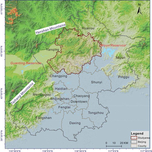
The study area is located in the Yanshan Mountains, at the intersection of Yanqing, Huairou, and Miyun Counties in northern Beijing (Figure 1), extending between latitude 40°14′–40°47′ and longitude 115°58′–116°50′. The terrain elevation in this study area varies from 182 m to 1534 m above the sea level, with a mean elevation of 587 m and a maximum slope gradient of 76.2° (calculated from DEM data).

Figure 1. Schematic of the study area location, which encompasses a variety of land cover types including forest, bare shrubs, plantations, residential, and earthen and tarmac roads. For full color versions of the figures in this article, please see the online version.

For this study, we acquired images recorded from two satellite sensors from the USGS (U.S. Geological Survey, access link: http://www.usgs.gov/): a Landsat 8 OLI image from 12 May 2013 and an EO-1 ALI L1G image from 1 May 2013. The Landsat 8 OLI image was the first OLI image of Beijing that was made publicly available for download. The solar elevation and solar azimuth angles for the two images were 62.82°, 138.63°, and 55.58°, 128.96°, respectively. The parameters for conversion of digital numbers (DN) to radiance (W ∙ m⁻² ∙ sr⁻¹ ∙ μm⁻¹) were also provided by the USGS. The satellite images were co-registered with the DEM by applying the new multitemporal matching algorithm (Pons, Moré, and Pesquer 2010). We also used ground control points (GCPs) to implement ortho-rectification, in which we obtained the accuracy of the subpixels. The main characteristics of the two sensors are presented in Table 2.

Table 2. Main characteristics of the OLI and ALI sensors.

	Landsat OLI spectral bands			EO-1 ALI spectral bands
	Bandwidth (μm)	GSD (m)		Bandwidth (μm)	GSD (m)
1	0.433–0.453	30	MS-1′	0.433–0.453	30
2	0.450–0.515	30	MS-1	0.450–0.515	30
3	0.525–0.600	30	MS-2	0.525–0.605	30
4	0.630–0.680	30	MS-3	0.630–0.690	30
–			MS-4	0.775–0.805	30
5	0.845–0.885	30	MS-4′	0.845–0.890	30
–			MS-5′	1.200–1.300	30
6	1.560–1.660	30	MS-5	1.550–1.750	30
7	2.100–2.300	30	MS-7	2.080–2.350	30
8	0.500–0.680	15	Pan	0.480–0.690	10
9	1.360–1.390	30

The DEM data with a resolution of 30 m was provided by the DLR (German: Deutsches Zentrum für Luft-und Raumfahrt e.V.) Earth Observation Center (downloaded from DLR FTP-Server at the German Remote Sensing Data Center, data link: ftp://taurus2.caf.dlr.de/).

2.5. Topographic correction

As a prerequisite, various model parameters must be computed prior to topographic correction. Thus, we randomly collected more than 5000 vegetation pixels in each band of the two satellite images from the study area. We then used the linear fitting methods described above to calculate the parameters C and k for all the image bands (Gao et al. 2014). The atmospheric transmittance values in this article are based on the results from Kaufman and Sendra (1988) and Chavez (1996) for the Landsat TM and ETM+ sensors. The AOT (τ) value was calculated using an evaluation by Moran et al. (1992), which was based on in-situ atmospheric measurements. To make further comparisons, we analyzed four typical Lambertian and non-Lambertian topographic correction models, including the cosine, the C-HuangWei, the SCS+C, and the Minnaert approaches.

3. Results

We evaluated the corrections by visual inspection and statistical and correlation analyses. The performance of these methods on remotely sensed images, with respect to differences in slope brightness, for instance, were observed qualitatively through visual inspection. Then, we compared the mean standard deviation (SD) reductions (%) of the pixel values of the different correction methods with the pixel values of the original image, and the results are presented in the statistical analysis section. The SD should decrease after successful correction, indicating that the impact of the topographic relief was reduced (Hantson and Chuvieco 2011). However, the most widely used method for validating the performance of image corrections is determining the decrease in the correlation between the illumination (cos i, as mentioned above) and the pixel values (Gao and Zhang 2009).

3.1. Visual contrast of topographic correction results

3.1.1. Sub-scene (a)

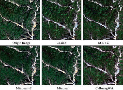
In the field of cartography, a long-standing convention in shade models is that the light comes from the northwest. In the field of remote sensing, however, the pseudoscopic effect is of particular importance, because most of the observation satellites that take images of the Earth’s surface have Sun-synchronous orbits. As a result, the images are captured when the illumination source is from the southeast (SE) direction, thereby causing the terrain reversal effect (Gil et al. 2014). Figure 2 shows sub-scene (a) of the Landsat 8 OLI image from the northern part of the study area. It has complex LULC, including a reservoir and shallows, a village, and other man-made structures. Elevations range from 200 m to 894 m, and slopes are under 37°. The true color map is a composite of OLI bands 4, 3, and 2, shown as red, green and blue for this area, respectively. The results reveal that the Minnaert-E correction ranked first, followed by the Minnaert, and then the SCS+C corrections. The cosine and the C-HuangWei corrections performed poorly due to overcorrection in the shadow of the mountains. However, the C-HuangWei correction had better color performance than the cosine correction.

Figure 2. Comparison of results from different models for sub-scene (a), RGB (OLI bands 4, 3, 2).

3.1.2. Sub-scene (b)

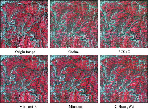
Figure 3 displays sub-scene (b) of the Landsat 8 OLI image from the center of the study area. It has the highest average height values of the three sub-scenes considered. Elevations range between 524 m and 1441 m, with slopes between 19.4° and 42.2°. There are many exposed rocks (white schistic patches in the original image) that are distributed especially in the sunny areas of the mountains. As we can see in Figure 3, clear strip lines appear in the correction results, particularly in the shadow areas of the mountains, except for those derived from the Minnaert and the Minnaert-E corrections. A comparison of the DEM and the change-detection results showed the DEM data to be very outdated, as this area has undergone many changes over the past 10 years, especially in the mountains along the road and the river. The corrections from the Minnaert and the improved Minnaert-E methods are not as sensitive to the DEM (or terrain) as the traditional methods. Our visual impression is that the Minnaert-E ranked first, followed by the Minnaert method.

Figure 3. Comparison of results from different models for sub-scene (b), RGB (OLI bands 5, 4, 3).

3.1.3. Sub-scene (c)

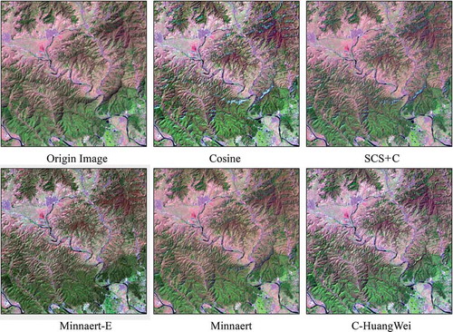
The sub-scene (c) calibration results of the topographic corrections are shown in Figure 4. This sub-scene contains the EO-1 ALI false color image composite bands MS-5, MS-4, and MS-2 as red, green and blue, respectively. Elevations in this area range between 25 m and 677 m, with slopes between 0° and 39.8°. Visually, all correction methods minimized the topographic effect to different degrees. However, obvious overcorrection was made by the cosine and the C-HuanWei corrections, which was mainly due to the defects of the Lambertian reflectance assumption (Gao et al. 2014). The corrections derived from the SCS+C, the Minnaert, and the improved model proposed in this article were distinctly improved, indicating that correction methods based on the non-Lambertian reflectance assumption perform better in rough terrain areas.

Figure 4. Comparison of results from different models for sub-scene (c), RGB (ALI bands MS-5, MS-4, MS-2).

3.2. Statistical analysis of topographic correction results

Tables 3 and 4 show a comparison of the mean SD reduction (%) of pixel values from the different correction methods with the pixel values from the original image. The results were generated from the correction of more than 3600 selected sample points in the vegetation coverage. As mentioned above, successful shade removal is indicated by a decrease in the SD value.

Table 3. Mean reduction (%) in SD, compared with the vegetation pixel values of the original image, after topographic correction on the Landsat 8 OLI image. The best algorithm performance results are in bold type.

Model name	Band 2	Band 3	Band 4	Band 5	Band 6	Band 7
Cosine	−7.2	2.3	−7.4	21.6	8.1	7.0
C-HuangWei	−13.9	−24.2	−13.1	14.0	−11.9	4.1
SCS+C	2.9	−7.5	−4.8	21.5	13.5	19.9
Minnaert	−4.4	9.3	12.9	25.6	13.1	−4.4
Minnaert-E	−2.7	15.5	16.7	24.0	16.9	15.31

Table 4. Mean reduction (%) in SD, compared with the vegetation pixel values of the original image, after topographic correction on the EO-1 ALI image. The best algorithm performance results are in bold type.

Model name	MS-1	MS-2	MS-3	MS-4′	MS-5	MS-7
Cosine	−6.0	1.9	−3.0	11.3	2.7	2.4
C-HuangWei	−6.9	−15.5	−6.8	−14.3	−16.8	−6.2
SCS+C	1.6	−5.5	1.6	10.2	11.0	3.3
Minnaert	−5.9	2.6	9.1	12.0	−1.4	−1.8
Minnaert-E	−0.5	10.4	17.2	19.2	10.6	10.2

First, we can see from Table 3 that the SD values increase after the cosine and C-HuangWei corrections, especially in the first three spectral bands. The higher SD values than those in the other methods indicate a more discrete distribution of the brightness values. Secondly, we observe that the SD values are reduced in the Minnaert correction results, and are similar to Minnaert-E correction SD values. Further comparison of these two correction methods shows that the Minnaert-E method performed better in the blue, green, red, and near-infrared spectra. Similar conclusions can be drawn from Table 4. The SD values after the cosine and C-HuangWei corrections again increased in the first three (visible) bands, and the improved Minnaert method performed best, with an average reduction of 10.7%.

In this study, we randomly chose more than 3600 sample points from the image stacks before and after correction. Tables 5 and 6 show the fitting results between the pixel and cos i values before and after topographic correction for two satellite images, respectively.

Table 5. The slope v and correlation coefficient r of the fitting results between OLI bands 2–7 pixel and cos i values. The radiance L was normalized to (0, 1) in order to avoid a large slope value v. The best algorithm performance results are in bold type.

Model name	Statistics	Band 2	Band 3	Band 4	Band 5	Band 6	Band 7
Original	v	0.25	0.36	0.33	0.59	0.27	0.20
	r	0.62	0.64	0.61	0.73	0.69	0.63
Cosine	v	−0.43	−0.37	−0.22	−0.32	−0.24	−0.21
	r	0.71	0.49	0.52	0.45	0.40	0.33
C-HuangWei	v	−0.37	−0.25	−0.15	−0.22	−0.19	−0.12
	r	0.62	0.66	0.55	0.56	0.49	0.37
SCS+C	v	0.10	0.21	0.48	0.25	0.16	0.15
	r	0.35	0.41	0.39	0.48	0.39	0.30
Minnaert	v	0.16	0.22	0.39	0.21	0.15	0.13
	r	0.41	0.48	0.39	0.32	0.41	0.33
Minnaert-E	v	0.12	0.16	0.22	0.18	0.13	0.20
	r	0.29	0.25	0.28	0.30	0.28	0.24

Table 6. The slope v and correlation coefficient r of the fitting results between EO-1 ALI bands pixel and cos i values. The radiance L was normalized to (0, 1) in order to avoid a large slope value v. The best algorithm performance results are in bold type.

Model name	Statistics	MS-1	MS-2	MS-3	MS-4′	MS-5	MS-7
Original	v	0.25	0.29	0.64	1.06	0.20	0.23
	r	0.43	0.52	0.34	0.31	0.25	0.30
Cosine	v	−0.67	−1.31	−1.66	−1.28	−0.28	−0.09
	r	0.23	0.35	0.27	0.26	0.20	0.13
C-HuangWei	v	−0.57	−0.87	−0.95	−0.63	−0.24	−0.33
	r	0.23	0.23	0.20	0.28	0.28	0.29
SCS+C	v	0.35	0.54	1.10	0.66	0.15	0.15
	r	0.46	0.35	0.27	0.26	0.13	0.25
Minnaert	v	0.28	0.25	0.45	0.24	0.55	0.12
	r	0.34	0.30	0.24	0.31	0.32	0.27
Minnaert-E	v	0.42	0.15	0.50	0.21	0.32	0.45
	r	0.22	0.19	0.18	0.22	0.25	0.22

As we see in Tables 5 and 6, the values for slope v and correlation coefficient r are high prior to correction. Compared with the other results, the fitting results derived from the cosine and C-HuangWei corrections are negative, due to overcorrection on the pixels with lower cos i values. This result is in agreement with the visual analysis results. The SCS+C method differs from the Minnaert correction only in areas with low cos i values, and it performs best among the three correction methods that are based on the Lambertian reflection assumption. The Minnaert method has both the lowest v and the lowest r values compared with the other correction methods. In addition, we found that the fitting results derived from all five correction methods for band 5 (MS-4ʹ) are distinctly higher than those from other bands, mainly because most of the sample points are in the vegetation coverage area. Band 7 (MS-7) has the lowest correlation coefficient between the pixel and the cos i values, compared with other bands and with the original image. This low correlation coefficient indicates that the corresponding spectrum of the 7th band is not as sensitive to the topographic relief as the 5th band.

Furthermore, the correlation analysis also indicates that methods based on non-Lambertian reflectance models can more effectively weaken the effects from topographic relief on surface radiance, which is consistent with the conclusions we made following visual inspection and statistical analysis. In Tables 5 and 6, we see that the Minnaert-E has the lowest slope and the lowest correlation coefficient between the corrected surface radiance (normalized) and the cos i values, which indicates that the proposed improved model performed better than the others. Based on the visual contrast and the correlation and statistical analyses results, we can confirm that the proposed Minnaert-E, based on non-Lambertian reflectance, is the best method of those tested in this article for topographically correcting OLI image and ALI image data.

4. Discussion

4.1. ρ calculation

For remote-sensing quantitative estimations based on reflectance and vegetation indices, the accuracy of the inversion model relies heavily on the processing of the remote sensing data, as well as on the determination of the input parameters (Guo, Chi, and Sun 2010; Fu et al. 2012; Gao et al. 2013). In a certain area, for instance, k may be a constant, but it may be possible, and discovered in the process of its calculation, that k partially depends on the solar incident angle (Gao et al. 2014). Ge et al. (2008) found that k values obtained by linear fitting under different degrees of slope gradient had obvious deviations. Thus the correction precision over a large region with relief must be further improved.

4.2. DEM effects and regression parameters

In the topography correction experiment of this study, the resolution of the DEM was 30 m, which is consistent with the resolution of the OLI data. In this case, resampling during the data process can thus be simply avoided in order to retain the entire original spectral information. However, the accuracy of the DLR SRTM x-band DEM is ±6 m (relative accuracy) and ±16 m (absolute accuracy), with a time lag of more than 10 years, compared to the satellite image. Conese et al. (1993) concluded that the accuracy of the DEM has a significant influence on the topography correction results. In our visual inspection in this study, the DEM effects were obvious in sub-scene (c). Li’s study (Li 2015) indicated that resolution has effects on the topographic relief derived from the DEM. However, there is no consensus as yet regarding the best combination of DEM and original image resolutions for topographic correction. In addition, terrain ups and downs are often associated with changes in the vertical distribution of vegetation, such as differences in vegetation at different slope angles and elevation levels, and different growth levels by the same vegetation. Otherwise, during the regression process for calculating the parameters, the selection of the random points has a fundamental impact on the final parameters obtained, and different sample point sets yielded regression parameters with certain differences. So, a more scientific approach for determining the regression parameters (such as k) must be further explored.

4.3. Correlation between the correction and slope gradient

In order to further ascertain suitable conditions for the Minnaert-E model, we can divide the remotely sensed image into four slope gradients in ascending order. We divided the random points selected in Section 2.5 into several groups according to slope gradient, then calculated the linear fitting results between the cos i and pixel values, respectively. We then plotted the correlation coefficient (r) of the regression equations, based on the slope gradient, after the Minnaert-E correction, as shown in Figure 5.

Figure 5. Fitting results along with the change of slope in each band. The correlation coefficient r of the fitting results between the OLI (a) and ALI (b) pixel and cos i values, respectively.

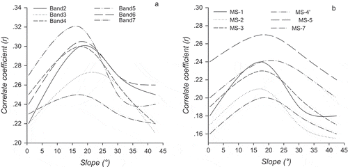
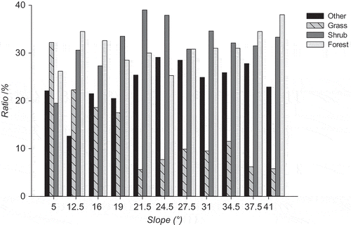
It is obvious that, for the visible bands of slope gradients within the study area (0°–43°), the correction result of Minnaert-E is not sensitive to the slope gradient (r is less than 0.3 for OLI and 0.24 for ALI). This shows that the Minnaert-E method can efficiently eliminate topography effects in the visible bands of the two sensors. For the second band, with a slope gradient of more than 30° (<43°), the r-curve extends under 0.26 and 0.17, respectively, which indicates a good topographic correction effect. In addition, for the 7th band, with a slope gradient of more than 25°, the r values of the fitting line are lower than 0.24. By plotting a statistical histogram of the slope gradients in the study area, we see that the regions in which the slope gradient ranges from 0° to 25° are widely distributed throughout the study area. With reference to the supervised classification results for different slope gradients in Figure 6, we can conclude that differences in LULC are the main reason for the fluctuations of the near-infrared band (4th band), which is more sensitive to the vegetation canopy and leaves (Wu et al. 2008).

Figure 6. Supervised classification results for different slope gradients.

As shown in Equation (11), the empirical coefficients method is still used in the Minnaert-E method to modify non-Lambertian reflection characteristics. In addition, we have assumed that sky scattering radiation is distributed isotropically, while in fact, sky scattering radiation has always been anisotropic. So the combination of a non-Lambertian reflection experience model with the bidirectional reflectance distribution theory to achieve improved results still requires further research.

5. Conclusion

In this article, we improved upon the Minnaert approach using transfer theory. We then used visual inspection and statistical and correlation analyses to comparatively evaluate the correction results for OLI and ALI multispectral images of the study area from five topographic correction models, including the improved Minnaert-E approach. Based on our results, we can draw the following conclusions:

1. Topographic correction models based on Lambertian reflectance theory were characterized by overcorrection, due to the neglect of reflection from sky diffusion and from the surrounding terrain. The weakness of the correction methods based on the non-Lambertian reflectance theory are also exposed in the presence of sky anisotropic scattering.

2. The proposed Minnaert-E approach, based on non-Lambertian reflectance theory, considers the complex radiation received by the Earth’s surface, which is derived from various radiation calculation methods with a rigorous theoretical foundation.

3. The proposed Minnaert-E model can effectively weaken the topographic effects caused by the topographic relief in slope gradients less than 10° and between 25° and 43°. It is clear that the Minnaert-E model is an efficient approach for topographic correction in terrain relief regions, especially for the regions with slope gradients less than 43°.

Acknowledgment

We thank both the USGS and DLR Earth Observation Center for their great efforts in developing and distributing the remotely sensed Landsat 8 satellite data and the SRTM X-SAR DEM data, and for their generosity in making these data available online at no cost.

Disclosure statement

No potential conflict of interest was reported by the authors.

ORCID

Mingliang Gao http://orcid.org/0000-0002-8871-6999

Additional information

Funding

This work was supported by the National Natural Science Foundation of China [grant 41130744], [grant number 41171335]; and the International Science & Technology Cooperation Program of China [grant number 2014DFA21620].

References

- Chavez, P. S. 1996. “Image-Based Atmospheric Correction-Revisited and Improved.” Photogrammetric Engineering and Remote Sensing 62 (9): 1025–1036.
- Chen, X. 2006. “Topographic Normalization of TM Imagery for Rock Classification in Pershing County, Nevada.” Accessed November 28, 2005. www.geo.wvu.edu/geog755/spring98/12/intro.htm
- Chen, H., and K. Cheng. 2012. “A Conceptual Model of Surface Reflectance Estimation for Satellite Remote Sensing Images Using in Situ Reference Data.” Remote Sensing 4 (12): 934–949. doi:10.3390/rs4040934.
- Civco, D. L. 1989. “Topographic Normalization of Landsat Thematic Mapper Digital Imagery.” Photogrammetric Engineering and Remote Sensing 55 (9): 1303–1309.
- Conese, C., M. A. Gilabert, F. Maselli, and L. Bottai. 1993. “Topographic Normalization of TM Scenes Through The Use of an Atmospheric Correction Method and Digital Terrain Models.” Photogrammetric Engineering and Remote Sensing 59 (12): 1745–1753.
- Dozier, J., and J. Frew. 1990. “Rapid Calculation of Terrain Parameters for Radiation Modeling from Digital Elevation Data.” IEEE Transactions on Geoscience and Remote Sensing 28 (5): 963–969. doi:10.1109/36.58986.
- Dymond, J. R., and J. D. Shepherd. 1999. “Correction of the Topographic Effect in Remote Sensing.” IEEE Transactions on Geoscience and Remote Sensing 37 (5): 2618–2619. doi:10.1109/36.789656.
- Ekstrand, S. 1996. “Landsat TM-Based Forest Damage Assessment: Correction for Topographic Effects.” Photogrammetric Engineering and Remote Sensing 62 (2): 51–161.
- Fu, X., G. H. Liu, C. Huang, and Q. S. Liu. 2012. “Remote Sensing Estimation Models of Suaeda Salsa Biomass in the Coastal Wetland.” Acta Ecologica Sinica 32 (17): 5355–5362 (in Chinese). doi:10.5846/stxb201201110062.
- Gao, M.-L., W.-J. Zhao, Z.-N. Gong, H.-L. Gong, Z. Chen, and X.-M. Tang. 2014. “Topographic Correction of ZY-3 Satellite Images and Its Effects on Estimation of Shrub Leaf Biomass in Mountainous Areas.” Remote Sensing 6 (4): 2745–2764. doi:10.3390/rs6042745.
- Gao, M. L., W. J. Zhao, Z. N. Gong, and X. H. He. 2013. “The Study of Vegetation Biomass Inversion Based on The HJ Satellite Data in Yellow River Wetland.” Acta Ecologica Sinica 33 (2): 542–553 (in Chinese). doi:10.5846/stxb201112051862.
- Gao, Y., and W. Zhang. 2009. “A Simple Empirical Topographic Correction Method for ETM+ Imagery.” International Journal of Remote Sensing 30 (9): 2259–2275. doi:10.1080/01431160802549336.
- Gao, Y. N., and W. C. Zhang. 2008. “Simplification and Modification of a Physical Topographic Correction Algorithm for Remotely Sensed Data.” Acta Geodaetica et Cartographica Sinica 37 (1): 89–94 (in Chinese).
- Ge, H., D. Lu, S. He, A. Xu, G. Zhou, and H. Du. 2008. “Pixel-Based Minnaert Correction Method for Reducing Topographic Effects on a Landsat 7 ETM+ Image.” Photogrammetric Engineering and Remote Sensing 74 (11): 1343–1350. doi:10.14358/PERS.74.11.1343.
- Gil, M., M. Arza, J. Ortiz, and A. Ávila. 2014. “DEM Shading Method for the Correction of Pseudoscopic Effect on Multi-Platform Satellite Imagery.” GIScience & Remote Sensing 51 (6): 630–643. doi:10.1080/15481603.2014.988433.
- Gu, D., and A. Gillespie. 1998. “Topographic Normalization of Landsat TM Images of Forest Based on Subpixel Sun-Canopy-Sensor Geometry.” Remote Sensing of Environment 64 (2): 166–175. doi:10.1016/S0034-4257(97)00177-6.
- Guo, Z. F., H. Chi, and G. Q. Sun. 2010. “Estimating Forest Aboveground Biomass Using HJ-1 Satellite CCD and ICESat GLAS Waveform Data.” Science China Earth Sciences 53 (S1): 16–25. doi:10.1007/s11430-010-4128-3.
- Hantson, S., and E. Chuvieco. 2011. “Evaluation of Different Topographic Correction Methods for Landsat Imagery.” International Journal of Applied Earth Observation and Geoinformation 13 (5): 691–700. doi:10.1016/j.jag.2011.05.001.
- Hay, J. E., and D. C. McKay. 1985. “Estimating Solar Irradiance on Inclined Surfaces: A Review and Assessment of Methodologies.” International Journal of Solar Energy 3 (4–5): 203–240. doi:10.1080/01425918508914395.
- Huang, W., L. P. Zhang, and P. X. Li. 2005. “An Improved Topographic Correction Approach for Satellite Image.” Journal of Image and Graphics 10 (9): 1124–1128 (in Chinese).
- Huang, W., L. P. Zhang, and P. X. Li. 2006. “A Topographic Correction Approach for Radiation of RS Images by Using Spatial Context Information.” Acta Geodaetica et Cartographica Sinica 35 (3): 285–290 (in Chinese).
- Kaufman, Y. J., and C. Sendra. 1988. “Algorithm for Automatic Atmospheric Corrections to Visible and Near-IR Satellite Imagery.” International Journal of Remote Sensing 9 (8): 1357–1381. doi:10.1080/01431168808954942.
- Law, K. H., and J. Nichol. 2004. “Topographic Correction for Differential Illumination Effects on IKONOS Satellite Imagery.” International Archives of Photogrammetry Remote Sensing and Spatial Information Sciences 35: 641–646.
- Li, M., J. Im, and C. Beier. 2013. “Machine Learning Approaches for Forest Classification and Change Analysis Using Multi-Temporal Landsat TM Images over Huntington Wildlife Forest.” GIScience & Remote Sensing 50 (4): 361–384.
- Li, Y. 2015. “Effects of Analytical Window and Resolution on Topographic Relief Derived Using Digital Elevation Models.” GIScience & Remote Sensing 52 (4): 462–477. doi:10.1080/15481603.2015.1049577.
- Moran, M. S., R. D. Jackson, P. N. Slater, and P. M. Teillet. 1992. “Evaluation of Simplified Procedures for Retrieval of Land Surface Reflectance Factors from Satellite Sensor Output.” Remote Sensing of Environment 41 (2–3): 169–184. doi:10.1016/0034-4257(92)90076-V.
- Pons, X., G. Moré, and L. Pesquer 2010. “Automatic Matching of Landsat Image Series to High Resolution Orthorectified Imagery.” Proceedings of the ESA Living Planet Symposium, Bergen, June 28–July 2. ESA Reference Document: SP-686.
- Reeder, D. H. 2002. Topographic Correction of Satellite Images: Theory and Application. New Hampshire: Dartmouth College.
- Richter, R., T. Kellenberger, and H. Kaufmann. 2009. “Comparison of Topographic Correction Methods.” Remote Sensing 1 (3): 184–196. doi:10.3390/rs1030184.
- Shi, D., G. J. Yang, and X. H. Mu. 2009. “Optical Remote Sensing Image Apparent Radiance Topographic Correction Physical Model.” Journal of Remote Sensing 13 (6): 1039–1046.
- Smith, J. A., T. L. Lin, and K. J. Ranson. 1980. “The Lambertian Assumption and Landsat Data.” Photogrammetric Engineering and Remote Sensing 46 (9): 1183–1189.
- Soenen, S. A., D. R. Peddle, and C. A. Coburn. 2005. “SCS+C: A Modified Sun-Canopy-Sensor Topographic Correction in Forested Terrain.” IEEE Transactions on Geoscience and Remote Sensing 43 (9): 2148–2159. doi:10.1109/TGRS.2005.852480.
- Teillet, P. M., B. Guindon, and D. G. Goodenough. 1982. “On The Slope-Aspect Correction of Multispectral Scanner Data.” Canadian Journal of Remote Sensing 8 (2): 84–106. doi:10.1080/07038992.1982.10855028.
- Vincini, M., D. Reeder, and E. Frazzi. 2002. “An Empirical Topographic Normalization Method for Forest TM Data.” Geoscience and Remote Sensing Symposium 4: 2091~2093. doi:10.1109/IGARSS.2002.1026454.
- Wen, J. G., Q. H. Liu, J. Xiao, Q. Liu, and X. W. Li. 2008. “A Model for Calculating the Optical Remote Sensing Reflectance in Complex Mountainous Area.” Scientia Sinica Terrae 38 (11): 1419–1427 (in Chinese).
- Wu, J. D., M. E. Bauer, D. Wang, and S. M. Manson. 2008. “A Comparison of Illumination Geometry-Based Methods for Topographic Correction of QuickBird Images of an Undulant Area.” ISPRS Journal of Photogrammetry and Remote Sensing 63 (2): 223–236. doi:10.1016/j.isprsjprs.2007.08.004.