Investigation of terrain illumination effects on vegetation indices and VI-derived phenological metrics in subtropical deciduous forests

Abstract

We used RapidEye and Moderate Resolution Imaging Spectroradiometer (MODIS)/Terra data to study terrain illumination effects on 3 vegetation indices (VIs) and 11 phenological metrics over seasonal deciduous forests in southern Brazil. We applied TIMESAT for the analysis of the Enhanced Vegetation Index (EVI) and the Normalized Difference Vegetation Index (NDVI) derived from the MOD13Q1 product to calculate phenological metrics. We related the VIs with the cosine of the incidence angle i (Cos i) and inspected percentage changes in VIs before and after topographic C-correction. The results showed that the EVI was more sensitive to seasonal changes in canopy biophysical attributes than the NDVI and Red-Edge NDVI, as indicated by analysis of non-topographically corrected RapidEye images from the summer and winter. On the other hand, the EVI was more sensitive to terrain illumination, presenting higher correlation coefficients with Cos i that decreased with reduction in the canopy background L factor. After C-correction, the RapidEye Red-Edge NDVI, NDVI, and EVI decreased 2%, 1%, and 13% over sunlit surfaces and increased up to 5%, 14%, and 89% over shaded surfaces, respectively. The EVI-related phenological metrics were also much more affected by topographic effects than the NDVI-derived metrics. From the set of 11 metrics, the 2 that described the period of lower photosynthetic activity and seasonal VI amplitude presented the largest correlation coefficients with Cos i. The results showed that terrain illumination is a factor of spectral variability in the seasonal analysis of phenological metrics, especially for VIs that are not spectrally normalized.

Keywords:

• vegetation indices
• topographic effects
• phenological metrics
• subtropical forests
• RapidEye
• MODIS

1. Introduction

Vegetation indices (VIs) and their derived phenological metrics (also known as seasonality parameters) are potential indicators of forest changes in response to climatic variations over time (Liang, Schwartz, and Fei 2011; Hmimina et al. 2013; Lambert et al. 2013; Du et al. 2014). However, as demonstrated in recent investigations using the Moderate Resolution Imaging Spectroradiometer (MODIS)/Terra (e.g., Morton et al. 2014; Maeda and Galvão 2015), there is still a need to understand better the potential factors that can affect the determination of the different VIs and the correct interpretation of the seasonal and interannual responses of vegetation.

VIs have distinct sensitivities to illumination effects due to canopy structure and sun-sensor geometry (Verrelst et al. 2008; Galvão et al. 2013). Several studies assume that topographic effects are minimal when VIs are expressed as band ratios, whereas others show that they are still significant (Song and Woodcock 2003; Verbyla, Kasischke, and Hoy 2008; Veraverbeke et al. 2010). In evergreen forests located over relatively flat terrains in the south Amazon, where the seasonal difference in the solar zenith angle (SZA) is close to 18º, the nadir-viewing MODIS Enhanced Vegetation Index (EVI) increases from the beginning to the end of the dry season with decreasing SZA (Galvão et al. 2011; Moura et al. 2012). In the south Amazon, the reduced amounts of canopy shadows viewed by the sensor toward the end of the dry season produce an increase in the near-infrared (NIR) reflectance as well as in the EVI. Therefore, the EVI increase in this region is not entirely associated with canopy photosynthetic activity. Another example of VI sensitivity was given by Matsushita et al. (2007) when studying high-density cypress plantations over mountains in Japan. They concluded that the EVI was more sensitive to topographic effects than the Normalized Difference Vegetation Index (NDVI). Thus, terrain illumination is a factor of spectral variability in phenological studies that has not been fully addressed in the literature.

In other important ecosystems of Brazil located at middle latitudes (e.g., the Atlantic Forest biome), seasonal differences in the SZA are much larger (>30º) than in the Amazon and topographic effects are commonly observed in satellite images (Ponzoni et al. 2014; Breunig et al. 2015). For example, as the season shifts from summer to winter over subtropical deciduous forests from southern Brazil, the SZA increases, the Leaf Area Index (LAI) decreases, and the local topography is highlighted for the satellite sensors. Therefore, the phenological response of the vegetation measured by the satellites will be affected to some extent by all of these factors.

In mountainous areas, topographic effects are more significant and affect the determination of canopy attributes, fractional vegetation cover, and net primary productivity (Combal and Isaka 2002; Huang et al. 2010). However, even in non-mountainous regions, the topography dissected by rivers valleys could affect the variability of VIs and phenological metrics. It occurs because of the different amounts of energy reflected seasonally toward the sensor by inclined surfaces in the forward and backscattering view directions.

Terrain illumination effects also depend on the spatial resolution of the sensors to hide (low spatial resolution) or highlight (high spatial resolution) topographic effects (Burgess, Lewis, and Muller 1995). MODIS is one of the sensors that best represents the state of the art in satellite phenological studies at coarse-to-moderate spatial resolution (Zhang et al. 2003; Soudani et al. 2012; Yuan, Wang, and Mitchell 2014). The MOD13Q1 product (MODIS/Terra Vegetation Indices 16-Day L3 Global 250-m SIN Grid V005) includes the NDVI and EVI. By using software such as TIMESAT (Jönsson and Eklundh 2004, 2012), several phenological metrics can be estimated from the MODIS VIs. We can inspect the sensitivity of these metrics to terrain illumination effects by topographic modeling of MODIS data. Despite the importance of terrain illumination, studies of its effects on MODIS TIMESAT phenological metrics derived from different VIs have not been reported in the literature.

With higher spatial resolution than MODIS, the RapidEye constellation of five satellites provides imagery over relatively large areas (swath of 77 km) with a revisit time of 5.5 days at nadir (Tyc et al. 2005; Kross et al. 2015). The satellites operate from a 630-km sun-synchronous orbit with a spatial resolution of 5 m. Each platform has a five-band push-broom instrument acquiring data in the visible and NIR spectral intervals, which allows the calculation of the NDVI and EVI. In addition, the chlorophyll-sensitive Red-Edge NDVI (Gitelson, Merzlyak, and Lichtenthaler 1996) can also be determined from RapidEye data. A strategy to improve the comprehension of the phenological variability of forests is to analyze MODIS product information in conjunction with that obtained from RapidEye data.

In this investigation, we used RapidEye and MODIS/Terra data acquired over seasonal deciduous forests from the Parque Estadual do Turvo (PET) in Brazil to study terrain illumination effects on 3 VIs (NDVI, EVI, and Red-Edge NDVI) and 11 TIMESAT phenological metrics. By using these two instruments, we investigated whether the topographic effects observed at a 5-m pixel size were still present in 250-m spatial resolution data. The sensitivity of each VI to the terrain illumination effects was analyzed before and after topographic correction over a study area with topography dissected by river valleys, altitudes ranging from 125 to 450 m, moderate-to-steep slopes (25–40º), and variable sun-facing (aspect) classes.

2. Study area

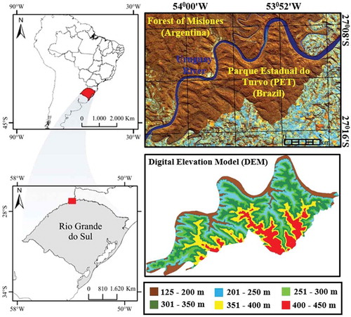
The PET (17,491 ha) is located in southern Brazil in the state of Rio Grande do Sul along the border with Argentina (Figure 1). The subtropical seasonal deciduous forest is part of the Atlantic Forest biome. The forest of the PET extends into the Forest of Misiones in Argentina (10,000 km²), which is separated from the PET by the Uruguay River (Brack et al. 1985). As shown in the 30-m digital elevation model (DEM) from the Shuttle Radar Topography Mission (SRTM), the amplitude of elevation reaches 325 m (Figure 1). Therefore, the PET is not located in a high-altitude mountainous area. It has undulating topography with areas dissected by river valleys. Moderate-to-steep slopes (25–40º) are observed close to the major rivers and streams. Surface orientation (aspect) is highly variable in the PET and east- to west-facing slopes are observed close to the Uruguay River (Figure 1). The major soil types are derived from basalts of the Paraná volcanic province.

Figure 1. Location of the Parque Estadual do Turvo (PET) in southern Brazil along the border with Argentina. The dissected relief of the park has an amplitude of 325 m, as indicated by the SRTM elevation data. For full color versions of the figures in this paper, please see the online version.

The climate type of the study area is humid subtropical (Cfa) in the Köppen classification with the highest and lowest mean temperatures observed in January (25°C) and July (13°C), respectively. In the coldest month, the temperatures may vary from −3ºC to 18ºC. The precipitation is regularly distributed over the months without a well-defined dry season. According to the inspection of gauge station data, most of the months have more than 100 mm of rainfall. The greatest amount of precipitation is generally observed in October (close to 250 mm), and the accumulated annual rainfall reaches 1600 mm (Breunig et al. 2015).

The predominant vegetation type (95% of the PET) is seasonal deciduous forest. From a vegetation map published by Guadagnin (1994), this forest type occurs over deep soil profiles in most of the PET and locally over shallower soil profiles close to the Uruguay River. From a floristic–structural survey performed in September 2013 over 14 sample plots (20 m × 50 m) in the northeastern portion of the park, we observed that the canopy structure of the seasonal deciduous forest has an emergent upper stratum formed by deciduous trees more than 20 m in height. The intermediate stratum is mainly composed of evergreen species and the lower stratum of young and low height trees. In agreement with previous surveys (e.g., Ruschel, Nodari, and Moerschbacher 2007), the average tree height and basal area were 11.53 ± 8.47 m and 21.92 ± 10.62 m²/ha, respectively. Most of the surveyed trees were less than 10 m in height, whereas 43% of them had heights between 10 and 20 m. Emergent trees (10%) were more than 20 m in height. The Shannon–Weaver Diversity Index (H), Pielou’s species evenness, and absolute density values were 3.58, 0.83, and 481 trees/ha, respectively.

3. Methodology

3.1. MODIS and RapidEye datasets

We used three pairs of orthorectified images (Level 3A) with a 5-m pixel size from four of the five available RapidEye satellites to represent the seasonal cycles of 2011, 2012, and 2013. As indicated in the last column of Table 1, the seasonal differences (amplitudes) in SZA during image acquisition ranged from 24º in 2013 to 33º in 2012. Most of the images were acquired at nadir (<10º view zenith angle – VZA), but some of them in 2011 and 2013 had VZAs between 10º and 13º. The following RapidEye bands were used in the data analysis: 1 (blue, 440–510 nm), 2 (green, 520–590 nm), 3 (red, 630–685 nm), 4 (red-edge, 690–730 nm), and 5 (NIR, 760–850 nm). The radiance data of these bands were converted into atmospherically corrected surface reflectance images using the Fast Line-of-Sight Atmospheric Analysis of Spectral Hypercubes (FLAASH), a MODTRAN4-based approach (Exelis 2013). We selected a Mid-latitude Summer atmospheric model with rural aerosols and visibility of 50 km.

Table 1. Dataset attributes for the three pairs of RapidEye images acquired in 2011, 2012, and 2013 in the Parque Estadual do Turvo (PET).

RapidEye satellite	Date of image acquisition	Season	Solar azimuth angle (º)	Solar zenith angle (º)	Difference in the solar zenith angle (º)
RE-1	6 March 2011	Summer	35	25	27
RE-2	15 June 2011	Autumn	13	52
RE-5	28 June 2012	Autumn	16	52	33
RE-1	17 October 2012	Spring	23	19
RE-2	28 February 2013	Summer	41	24	24
RE-4	1 August 2013	Winter	22	48

Two MODIS products were used in the data analysis. They were converted from sinusoidal projection to planar coordinates using the MODIS Reprojection Tool algorithm (Dwyer and Schmidt 2006). The first product was the MOD13Q1, which was chosen to obtain the phenological metrics. This composite product was selected to reduce the spectral variability due to atmospheric and view angle effects. It includes 250-m, 16-day EVI and NDVI data as well as information on VZAs/SZAs and pixel quality retrievals. EVI was proposed to reduce atmospheric and soil background influences on NDVI and to be more sensitive to canopy biophysical attributes (Huete et al. 2002).

The second product was the MOD15A2 (MODIS/Terra Leaf Area Index/FPAR 8-Day L4 Global 1 km SIN GridV005) (Myneni et al. 2002; Tan et al. 2005). It provided ancillary LAI data to compensate for the absence of ground information on seasonal LAI changes. Only the highest quality LAI retrievals calculated from the 3D-radiative transfer main algorithm were used.

3.2. Vegetation indices and MODIS TIMESAT phenological metrics

The VIs calculated from the RapidEye data were the NDVI [Equation (1)], Red-Edge NDVI [Equation (2)], and EVI [Equation (3)]:

(1)

(2)

(3)

where ρ_NIR, ρ_red-edge, ρ_red, and ρ_blue comprise the reflectance of the RapidEye bands 5, 4, 3, and 1, respectively; G (2.5) is a scaling factor; L (1.0) is the canopy background adjustment factor; and C₁ (6.0) and C₂ (7.5) are the coefficients of the aerosol resistance term (Solano et al. 2010).

We applied TIMESAT 3.1 (Jönsson and Eklundh 2012) to calculate phenological metrics from the MODIS EVI and NDVI (MOD13Q1 product) for the growing season that spanned over 2011 and 2012. TIMESAT is based on least-squares fits to the upper envelope of the VI data. It was described in detail by Jönsson and Eklundh (2004). From three available methods in TIMESAT, which generally present similar results (Hird and Mcdermid 2009), we chose the asymmetric Gaussian method. It is less sensitive to noise in the time series when compared to Savitzky–Golay filtering (Jönsson and Eklundh 2012). We assigned weights for pixel quality control using the MOD13Q1 pixel reliability information. Weights of 1.0, 0.5, and zero were used to represent good (code zero in pixel reliability), marginal (code 1), and cloudy data (code 3), respectively.

From the fitted model functions, 11 phenological metrics with different ecological meanings were calculated on a per-pixel basis. The metrics, described by Jönsson and Eklundh (2004, 2012), were as follows: Start of Season (SOS), End of Season (EOS), Length of Season (LOS), Base Level (BL), Maximum of Fitted VI Value (MV), Time of Mid of the Season (TMS), Seasonal Amplitude (SA), Left Derivative (LD), Right Derivative (RD), Large Integral (LInt), and Small Integral (SInt).

3.3. Terrain illumination effects

Non-Lambertian methods generally have better performance in removing topographic effects than Lambertian methods because they are band-specific approaches (Goslee 2012). In this study, we focus on the non-Lambertian C-correction of the RapidEye data. The technique is based on the cosine of the solar incidence angle i, which is the angle between a vector pointed toward the sun and a vector normal to the surface (Teillet, Guindon, and Goodenough 1982). Cos i was calculated as follows [Equation (4)]:

(4)

where θ_s is the solar elevation, θ_t is the slope, φ_s is the solar azimuth, and φ_t is the aspect.

Topographical slope and aspect data were derived from 30-m SRTM elevation data resampled to and co-registered with the RapidEye images. The terrain-corrected surface reflectance (ρ_t) of the RapidEye images using the C-correction technique was obtained by Equation (5):

(5)

where ρ_s is the surface reflectance of each RapidEye band, θ_z is the SZA, and i is the incidence angle. The parameter C_k is band specific and was determined from Equation (6):

(6)

where b_k and m_k are the respective intercept and slope of the regression relationships between Cos i and the ρ_s of each band.

To obtain C_k, a random stratified sampling approach by Cos i was adopted, selecting 200 pixels in the RapidEye images to represent the entire range of shaded (Cos i close to zero) and sunlit (close to 1) surfaces. According to Reese and Olsson (2011), topographic C-correction using random stratified sampling approaches by Cos i provides better results than random sampling strategies.

The performance of the topographic correction was assessed by two steps. First, we calculated correlation coefficients (r) between the reflectance of the RapidEye bands and Cos i, before and after C-correction. This is the most widely used method for validating the performance of the topographic correction (Gao and Zhang 2009). In the second step, we used the vegetation map from Guadagnin (1994) to select sites of seasonal deciduous forests over deep and shallow soil profiles having distinct aspect and slope attributes. We compared their mean reflectance (n = 50 pixels) before and after topographic correction. Box–whisker plots were generated and two-sample t-tests for mean differences were performed at the 0.05 significance level.

To investigate the terrain illumination effects on RapidEye VIs, we calculated the percentage difference before and after topographic correction. We inspected RapidEye reflectance spectra from sunlit and shaded surfaces over the selected sites, before and after C-correction, and correlated the VIs with Cos i. The influence of the C₁, C₂, and L parameters of the EVI [Equation (3)] on the terrain illumination effects was investigated by fixing one parameter while varying the others. First, we fixed L at 1.0 and changed each of the C parameters from zero to 10. Then, we kept C₁ and C₂ fixed at 6.0 and 7.5, respectively, and simulated L from zero to 1.0. Pearson’s correlation coefficients between the EVI and Cos i were obtained at each step of simulation.

Finally, we used MODIS data to verify whether the topographic effects detected at a 5-m spatial resolution were still present at coarse-to-moderate spatial resolution (250 m). To obtain the Cos i image, we used the SZA (57º) and azimuth (27º) angle to represent the MODIS data acquired in the winter (1 July 2012) when great amounts of shadows are observed in the scene. We compared the Cos i image with the images obtained from the 11 TIMESAT phenological metrics calculated from the MODIS EVI and NDVI. To identify the most affected metrics by topographic effects, we correlated the values of each metric with Cos i using 100 pixels selected over different poorly and well-illuminated surfaces.

4. Results

4.1. Seasonal variations in LAI, SZA, and VIs

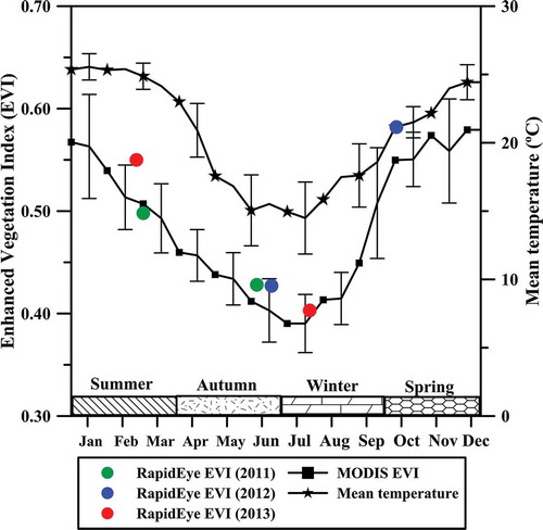
At the time of MODIS data acquisition over the PET, the SZA increased from summer (22º) to winter (55º) (Figure 2). On the other hand, the average LAI of the seasonal deciduous forest decreased from 6.0 to 4.0, as indicated from inspection of the MOD15A2 product (Figure 2). Both factors (LAI and SZA) produced a MODIS and RapidEye VI decrease due to deciduousness and the influence of canopy/terrain shadows for the sensors. The MODIS and RapidEye EVI data followed the general seasonal pattern of temperature showing mean values close to 0.55 in the summer and 0.40 in the winter (Figure 3).

Figure 2. LAI estimates from the MOD15A2 product, averaged between 2002 and 2012 (n = 50 pixels). The seasonal variation in the solar zenith angle (SZA) from the MODIS data is also shown.

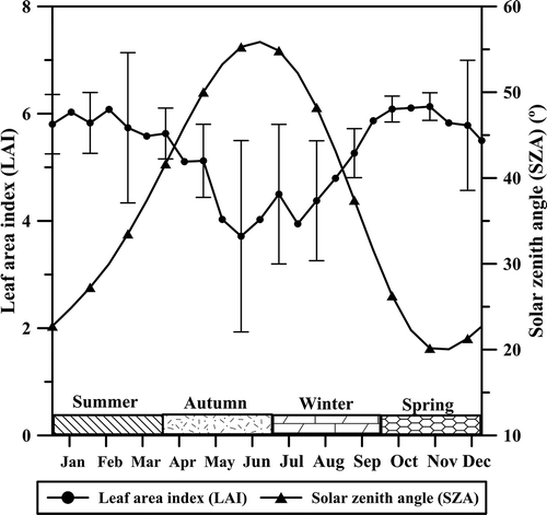
Figure 3. Seasonal variations in average MODIS EVI and temperature (gauge station). Average EVI values for the three pairs of RapidEye images obtained in 2011, 2012, and 2013 are also indicated.

For the three pairs of RapidEye images listed in Table 1, the seasonal SZA difference between 24º and 33º produced important differences in terrain illumination or reflectance for the sensor. For example, shadows predominated along the dissected relief of the PET, especially in the valleys, from March (SZA = 25º) to June (SZA = 52º) of 2011 (Figure 4). On the other hand, close to the Uruguay River, a small number of sunlit surfaces facing to the east were topographically enhanced in the winter [Figure 4(b)] compared to summer [Figure 4(a)]. For the three pairs of dates under analysis, the RapidEye NDVI, Red-Edge NDVI, and EVI showed lower values for sunlit and shaded surfaces with the seasonal decrease in LAI and the increase in SZA (Figure 5).

Figure 4. Seasonal variations in surface reflectance with increasing solar zenith angle (SZA) and decreasing Leaf Area Index (LAI) from the (a) summer to (b) autumn of 2011. The RapidEye bands 5 (760–850 nm), 4 (690–730 nm), and 3 630–685 nm) are displayed in red, green, and blue, respectively.

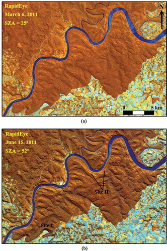
Figure 5. Seasonal variations in NDVI, Red-Edge NDVI, and EVI for non-topographically corrected RapidEye images acquired in the summer (28 February) and winter (1 August) of 2013.

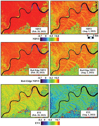
In 2013, seasonal differences in the RapidEye NDVI due to changes in biophysical attributes and illumination effects (SZA = 24º) resulted in a percentage decrease of 9% for most of the seasonal deciduous forest of the PET and between 10% and 19% over their shaded surfaces. When compared with the NDVI and Red-Edge NDVI (results not shown), the EVI was much more sensitive to LAI and canopy/terrain shadows. From the summer to winter, the EVI had a percentage decrease predominantly between 20% and 39%. Changes greater than 40% produced a better delineation of the local topography (Figure 5).

4.2. Assessment of the topographic correction

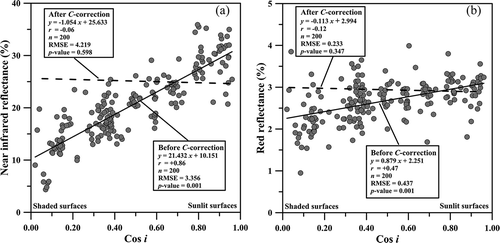
During the evaluation of the performance of the C-correction technique, the reflectance of all RapidEye bands showed positive correlation coefficients with Cos i that decreased after topographic correction (Figure 6). The coefficients were higher in the NIR band 5 [r = + 0.86 in Figure 6(a)] and lower toward the red-edge band 4 (r = + 0.81) and, especially, the visible bands [e.g., r of +0.45 for the red band 3 in Figure 6(b)]. After applying the C-correction technique, the slope of the regression relationships decreased to values close to zero, as indicated by the dashed fit lines in Figure 6. As a result, topographic features were suppressed in the terrain-corrected RapidEye images compared to the non-corrected data.

Figure 6. Relationships of the cosine of the incidence angle i with the (a) near-infrared and (b) red reflectance of seasonal deciduous forest for the RapidEye data acquired in 1 August 2013 (SZA = 48º). The relationships after topographic correction are indicated by the dashed fit lines. Symbols are omitted for better graphic representation.

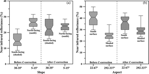
Additionally, to confirm the performance of topographic correction, we evaluated two sites (“I” and “II”) with locations shown in Figure 4(b). They have the same vegetation type but present distinct slope and aspect values. Site I is composed of the predominant seasonal deciduous forest in the PET with well-developed canopy strata over deep soil profiles (Guadagnin 1994). Compared with site I, the seasonal deciduous forest that occurs over shallower soils in site II does not have a well-defined upper stratum. Therefore, the spectral response of the vegetation of site II is much more influenced by vegetation species from the intermediate-to-lower herbaceous strata than from the upper stratum.

For site I, NIR reflectance differences between sunlit and shaded surfaces were reduced after C-correction, as illustrated by box–whisker plots [Figure 7(a)]. Two-sample t-tests showed that the NIR reflectance differences between the means of these surfaces were statistically significant before C-correction and not significant after C-correction at the 0.05 level, as expected. On the other hand, the shaded surfaces became more heterogeneous after topographic correction, which was associated with overcorrection of the NIR reflectance of some pixels. For site II, reflectance differences between the east- and west-facing slopes were also reduced after topographic correction, but they were still statistically significant at the 0.05 level [Figure 7(b)]. This may indicate undercorrection of the NIR reflectance of the sunlit surface.

Figure 7. Box–whisker plots before and after topographic correction of the near-infrared reflectance of RapidEye band 5 for seasonal deciduous forests with (a) distinct slope and aspect values (site I) and (b) opposite aspect and slope ranging from 15º to 25º (site II). Endpoints of the whiskers represent 10/90 percentile.

4.3. Terrain illumination effects on RapidEye vegetation indices

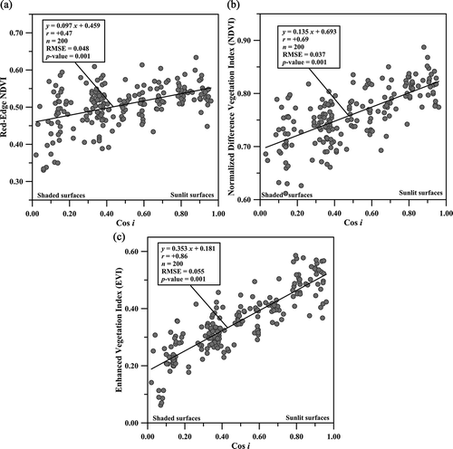
The terrain illumination effects were stronger on the EVI of the seasonal deciduous forest in the PET, as expressed by the correlation between each VI and Cos i. The correlation coefficients increased from the RapidEye Red-Edge NDVI (r = + 0.47) and NDVI (r = + 0.69) to the EVI (r = + 0.86), as shown in Figure 8(a)–(c), respectively. Therefore, all VIs increased from shaded to sunlit surfaces with increasing Cos i values.

Figure 8. Relationships of the cosine of the incidence angle i with the (a) Red-Edge NDVI, (b) NDVI, and (c) EVI calculated from RapidEye data acquired over seasonal deciduous forest in 1 August 2013 (SZA = 48º).

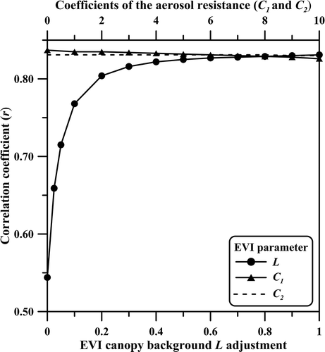
Because of the larger sensitivity of the EVI to topographic effects, we investigated the influence of the L and C parameters of Equation (3) on the EVI behavior. When we kept C₁ and C₂ constant and varied L, we observed a decrease in the correlations between the EVI and Cos i for L values lower than 0.5. The decrease in L reduced the EVI dependence on topography, whereas the changes in the C parameters had no influence on the terrain illumination effects (Figure 9).

Figure 9. Influence of the aerosol resistance coefficients (C₁ and C₂) and canopy background L adjustment parameter to reduce terrain illumination effects on the EVI. The effects are expressed by correlations between EVI and Cos i.

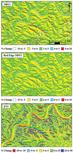
From the percentage change results between terrain-corrected and non-corrected RapidEye data acquired in 1 August 2013, we observed that the Red-Edge NDVI was less sensitive to topographic effects than the NDVI, at least over shaded surfaces. This was indicated by the smaller number of pixels in red (6–10% of change) observed in the Red-Edge NDVI image of Figure 10. On the other hand, strong changes in EVI were observed along the dissected relief of the PET after C-correction. In the percentage difference EVI image of Figure 10, sunlit surfaces showed an EVI decrease up to 20% (red) after topographic correction, whereas the shaded surfaces presented an EVI increase up to 90% (blue).

Figure 10. Percentage change in NDVI, Red-Edge NDVI, and EVI between terrain-corrected and non-corrected RapidEye data acquired in 1 August 2013, with a solar zenith angle (SZA) of 48º.

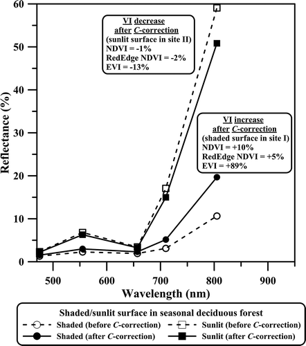
We plotted RapidEye spectra extracted from poorly and well-illuminated pixels over sites I and II indicated in Figure 4(b). After C-correction, shaded surfaces (Cos i = 0.1) showed a reflectance increase, while sunlit surfaces (Cos i = 0.9) showed a reflectance decrease (Figure 11). The absolute reflectance differences after C-correction were stronger in the NIR. Consequently, due to the higher NIR dependence and non-normalization of the bands, the EVI presented the greatest percentage changes after topographic correction for both the shaded and the sunlit surfaces. Over the shaded surfaces, the percentage increase was 89%, 14%, and 5% for the EVI, NDVI, and Red-Edge NDVI, respectively (Figure 11). Over the sunlit surfaces, the decrease was of 13%, 1%, and 2%, respectively.

Figure 11. Changes in RapidEye surface reflectance spectra over sunlit and shaded surfaces before (dashed lines) and after (thick lines) topographic correction. The percentage change for each vegetation index after C-correction is indicated.

4.4. Terrain illumination effects on MODIS phenological metrics

The MODIS Cos i image obtained from the SRTM–DEM with SZA and azimuth angles of 57º and 27º still showed some shaded and sunlit surfaces in dark and bright pixels, respectively. These angles correspond to MODIS data acquired in the winter (1 July). Therefore, when we obtained the Cos i image at the MODIS spatial resolution, we noted that the topographic features observed in the RapidEye images (5 m) from the winter were not entirely aggregated at the coarse-to-moderate spatial resolution of 250 m.

Terrain illumination affected 6 of the 11 TIMESAT phenological metrics in the growing season that spanned over 2011 and 2012, especially the metrics derived from the EVI. The results showed that the EVI-derived BL and SA metrics were more strongly impacted by terrain illumination than the MV, LD, RD, Lint, and SInt metrics, as expressed by the largest correlation coefficients with Cos i (Table 2). In Table 2, the correlations increased from the NDVI to EVI phenological metrics, confirming the greater sensitivity of the EVI-derived phenological metrics to the terrain illumination effects. In contrast, SOS, EOS, LOS, and TMS were less sensitive to topographic effects, having poor correlations with Cos i for both VIs.

Table 2. Pearson’s correlation coefficients (r) between the cosine of the incidence angle (Cos i) and 11 TIMESAT phenological metrics calculated from the MODIS NDVI and EVI in the 2011/2012 growing season.

MODIS phenological metrics	NDVI (r)	EVI (r)
Start of Season (SOS)	−0.14	+0.13
End of Season (EOS)	+0.29	+0.01
Length of Season (LOS)	+0.26	+0.00
Base Level (BL)	+0.51*	+0.89*
Time of Mid of the Season (TMS)	+0.03	−0.27
Maximum Value (MV)	+0.39	+0.65*
Seasonal Amplitude (SA)	−0.51*	−0.82*
Left Derivative (LD)	−0.36	−0.76*
Right Derivative (RD)	−0.50*	−0.65*
Large Integral (LInt)	+0.35	+0.43
Small Integral (SInt)	−0.46	−0.78*

Note: *Significant at the 0.01 level.

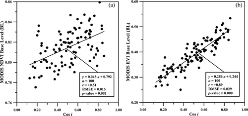
In the TIMESAT software, BL is the average of the left and right minimum VI values, representing the period of lower photosynthetic activity. Thus, it is the baseline composed of the average minimum VI values observed in our study area in the autumn (left minimum VI) and winter (right minimum VI). As expected from previous results with RapidEye, this baseline will be shifted from poorly to well-illuminated terrain. For instance, in the 2011/2012 growing season, the EVI-derived BL increased from shaded (red in Figure 12) to sunlit (green) surfaces, showing a positive correlation with Cos i. As illustrated in Figure 13(a) and 13(b), the relationships for BL were linear and increased from NDVI (r = + 0.51) to EVI metrics (r = + 0.89). On the other hand, SA increased from sunlit to shaded surfaces, presenting an inverse relationship with Cos i (r = −0.82) (Table 2). SA is the difference between the maximum VI and BL, indicating the seasonal variation of photosynthetic activity. In other words, the amplitude between the maximum EVI value of summer and the baseline defined by minimum EVI values of autumn and winter were greater over shaded surfaces than over sunlit terrains in the deciduous forest of the PET, which is consistent with results obtained for BL. It should be the same over similar physiognomies if not affected by topographic effects.

Figure 12. Terrain illumination effects on the MODIS EVI-derived base level (BL) metric, calculated from the 2011/2012 growing season using TIMESAT.

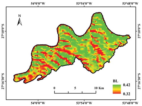
Figure 13. Relationships of Cos i with the base level (BL) metric derived from the MODIS (a) NDVI and (b) EVI.

5. Discussion

Terrain illumination effects depend on the selected VI, view-illumination geometry, spatial resolution, and type of vegetation and relief. Even in non-mountainous areas with dissected relief such as in the PET, terrain illumination is an important factor of spectral variability in the seasonal analysis of phenological metrics when the satellite data are acquired under large seasonal variation in the SZA. In our study area, terrain illumination effects were observed at both high- and coarse-to-moderate spatial resolution and were stronger for the EVI than for the NDVI and Red-Edge NDVI. The MODIS EVI-derived TIMESAT metrics were also much more affected by topographic effects than the NDVI-derived metrics, especially the metrics associated with the period of lower photosynthetic activity and seasonal amplitude (BL and SA). Metrics related to the maximum EVI value or to derivatives or integrals were also influenced by changes in sunlit and shaded surfaces.

The greater sensitivity of the EVI to topographic effects is explained by two major factors. First, when compared to the NDVI and Red-Edge NDVI, the EVI does not behave as a normalized difference or a ratio-based VI that can reduce topographic effects. Second, the three-band EVI is mainly driven by the single NIR reflectance (r = + 0.99 in this study), which is the RapidEye band most correlated with Cos i. In the NIR, the foliage efficiently scatters photons and the EVI is more sensitive to LAI (Moura et al. 2012; Peng, Gitelson, and Sakamoto 2013; Breunig et al. 2015). On the other hand, due to both factors, the EVI is also much more affected by shadows or view-illumination geometry than the other indices (Galvão et al. 2011; Morton et al. 2014).

The influence of shadows on this index was demonstrated in previous studies by Anderson et al. (2011) and Galvão et al. (2011), who found a strong inverse correlation between the EVI and the shade fraction from spectral mixture modeling of MODIS and hyperspectral Hyperion data in the Amazon, respectively. According to Peng, Gitelson, and Sakamoto (2013), the EVI over crops behaves as a difference between the NIR and red reflectance rather than a normalized difference. In Japanese cypress plantations, Matsushita et al. (2007) noted that the topographic effects on the EVI could not be ignored, especially because of the canopy background adjustment factor L. In our study, we observed a decrease in the correlations between the EVI and Cos i for L values lower than 0.5. The decrease in L will reduce the topographic influence over seasonal deciduous forests of the study area, but it will probably also decrease the EVI sensitivity to LAI. The deciduousness in the PET is mainly controlled by the temperature or photoperiod because the precipitation is regular throughout the year. The LAI decrease of some deciduous species is also associated with lower temperatures in the winter that make water absorption by the roots difficult, producing a hydric deficit even with the availability of water in the soil horizons (Franco 2008). That was the reason that the MODIS and RapidEye VIs followed the general seasonal pattern of temperature in this study, decreasing from the summer to winter.

Several techniques for topographic correction have been proposed in the literature, and there is no consensus on the best technique (Wu et al. 2008; Richter, Kellenberger, and Kaufmann 2009; Veraverbeke et al. 2010; Gil et al. 2014). Different strategies to assess the quality of the topographic correction have also been considered, including the evaluation of classification accuracy of land covers and the estimates of biophysical attributes before and after correction (Huang et al. 2010; Ediriweera et al. 2013; Li, Im, and Beier 2013; Moreira and Valeriano 2014). The performance of the topographic correction varies with the land cover types, terrain spatial heterogeneity, and DEM spatial scale. The dependence of topographic correction on the DEM spatial scale increases with the complexity of the terrain (Zhang, Yan, and Bai 2015). In our study, the C-correction of topographic effects using a 30-m DEM was facilitated by the predominance of a single forest type in the PET. The observed reflectance increase of the RapidEye bands with increasing Cos i values was consistent with previous studies (Soenen et al. 2008; Wu et al. 2008). The correlation between the reflectance and Cos i was positive for all RapidEye bands and decreased from the NIR to the visible bands, as was also observed in other investigations using Landsat data (Veraverbeke et al. 2010). Correlation coefficients decreased after C-correction of the RapidEye data to values close to zero, an indication of successful topographic correction (Gao and Zhang 2009). The standard deviation of the reflectance should decrease after a successful shade removal (Hantson and Chuvieco 2011; Balthazar et al. 2012). Detailed analysis of selected sites in the PET using box–whisker plots showed reduction of the standard deviation for some surfaces and increase for other terrains after topographic correction, which was associated with outliers and overcorrected or undercorrected pixels.

Our results indicate that topographic effects are important in the intraannual analysis of the EVI phenological metrics calculated on a per-pixel basis using large field-of-view instruments (e.g., MODIS) or sensors with pointing capability (e.g., RapidEye). The effects may also affect the correct interpretation of seasonality parameters during interannual analyses of off-nadir data. The SZA is not a source of variability in the interannual analysis of the EVI. However, changes in VZA modify the amounts of energy reflected seasonally in the NIR toward the sensors by surfaces having different slope and aspect values. Consequently, the EVI of these surfaces will also change across years with variations in VZA.

6. Conclusions

We analyzed terrain illumination effects on 3 VIs and 11 phenological metrics over seasonal deciduous forests in southern Brazil. The results showed strong changes in the RapidEye EVI in the winter, along the dissected relief of the PET, after C-correction of topographic effects. Because the reflectance decreased over sunlit surfaces and increased over shaded surfaces, especially in the NIR, the three VIs had similar behavior after topographic correction. The Red-Edge NDVI, NDVI, and EVI decreased up to 2%, 1%, and 13% over sunlit surfaces and increased up to 5%, 14%, and 89% over shaded surfaces, respectively. Topographic effects affected also the seasonal analysis of the 250-m MODIS data, confirming the greater sensitivity of the EVI-derived TIMESAT metrics compared with the NDVI seasonality parameters. The metrics BL and SA, followed by MV, LD, RD, Lint, and SInt, were correlated with Cos i. They were more affected by terrain illumination than SOS, EOS, LOS, and TMS.

Therefore, although the EVI was more sensitive to canopy biophysical attributes (e.g., LAI) than the NDVI and Red-Edge NDVI in non-corrected topographic data, it was much more affected by terrain illumination effects. This occurs because this three-band VI is mainly driven by the NIR reflectance, which is highly correlated with Cos i, and by changes in the canopy background L parameter. Furthermore, EVI does not behave as a normalized difference or ratio-based VI to compensate for variations in illumination of the scene.

Acknowledgments

MODIS data were provided by the Land Processes Distributed Active Archive Center (LPDAAC). The comments by the anonymous reviewers are highly appreciated.

Disclosure statement

No potential conflict of interest was reported by the author(s).

Additional information

Funding

This research was funded by the Fundação de Amparo à Pesquisa do Estado de São Paulo (FAPESP) [grant number 2013/03908-3]. The authors are also grateful to Conselho Nacional de Desenvolvimento Científico e Tecnológico (CNPq) [grant number 168869/2014-4], [grant number 305914/2014-6]; and Coordenação de Aperfeiçoamento de Pessoal de Nível Superior (CAPES).

References

- Anderson, L. O., L. Aragão, Y. E. Shimabukuro, S. Almeida, and A. Huete. 2011. “Fraction Images for Monitoring Intra-Annual Phenology of Different Vegetation Physiognomies in Amazonia.” International Journal of Remote Sensing 32: 387–408. doi:10.1080/01431160903474921.
- Balthazar, V., V. Vanacker, and E. F. Lambin. 2012. “Evaluation and Parameterization of ATCOR3 Topographic Correction Method for Forest Cover Mapping in Mountain Areas.” International Journal of Applied Earth Observation and Geoinformation 18: 436–450. doi:10.1016/j.jag.2012.03.010.
- Brack, P., R. M. Bueno, M. R. C. D. B. Falkenberg, M. R. C. Paiva, M. Sobral, and J. R. Stehmann. 1985. “Levantamento florístico do Parque Estadual do Turvo, Tenente Portela, Rio Grande do Sul, Brasil.” Roessléria 7: 69–94.
- Breunig, F. M., L. S. Galvão, J. R. Santos, A. A. Gitelson, Y. M. Moura, T. S. Teles, and W. Gaida. 2015. “Spectral Anisotropy of Subtropical Deciduous Forest Using MISR and MODIS Data Acquired under Large Seasonal Variation in Solar Zenith Angle.” International Journal of Applied Earth Observation and Geoinformation 35: 294–304. doi:10.1016/j.jag.2014.09.017.
- Burgess, D. W., P. Lewis, and J.-P. A. L. Muller. 1995. “Topographic Effects in AVHRR NDVI Data.” Remote Sensing of Environment 54: 223–232. doi:10.1016/0034-4257(95)00155-7.
- Combal, B., and H. Isaka. 2002. “The Effect of Small Topographic Variations on Reflectance.” IEEE Transactions on Geoscience and Remote Sensing 40: 663–670. doi:10.1109/TGRS.2002.1000325.
- Du, J., Z. He, J. Yang, L. Chen, and X. Zhu. 2014. “Detecting the Effects of Climate Change on Canopy Phenology in Coniferous Forests in Semi-Arid Mountain Regions of China.” International Journal of Remote Sensing 35: 6490–6507. doi:10.1080/01431161.2014.955146.
- Dwyer, J., and G. Schmidt. 2006. “The MODIS Reprojection Tool.” In Earth Science Satellite Remote Sensing, Eds. J. J. Qu, W. Gao, M. Kafatos, R. E. Murphy, and V. V. Salomonson, 162–177. Berlin, Heidelberg: Springer.
- Ediriweera, S., S. Pathirana, T. Danaher, D. Nichols, and T. Moffiet. 2013. “Evaluation of Different Topographic Corrections for Landsat TM Data by Prediction of Foliage Projective Cover (FPC) in Topographically Complex Landscapes.” Remote Sensing 5: 6767–6789. doi:10.3390/rs5126767.
- Exelis Visual Information Solutions. 2013. “Environment for Visualizing Images (ENVI).” Version 5.0.
- Franco, A. M. S. 2008. “Estrutura, diversidade e aspectos ecológicos do componente arbustivo e arbóreo em uma floresta estacional, Parque estadual do Turvo, Sul do Brasil.” PhD diss., Universidade Federal do Rio Grande do Sul, Porto Alegre, RS, Brasil. 82 p.
- Galvão, L. S., F. M. Breunig, J. R. Santos, and Y. M. Moura. 2013. “View-Illumination Effects on Hyperspectral Vegetation Indices in the Amazonian Tropical Forest.” International Journal of Applied Earth Observation and Geoinformation 21: 291–300. doi:10.1016/j.jag.2012.07.005.
- Galvão, L. S., J. R. Santos, D. A. Roberts, F. M. Breunig, M. Toomey, and Y. M. Moura. 2011. “On Intra-Annual EVI Variability in the Dry Season of Tropical Forest: A Case Study with MODIS and Hyperspectral Data.” Remote Sensing of Environment 115: 2350–2359. doi:10.1016/j.rse.2011.04.035.
- Gao, Y., and W. Zhang. 2009. “A Simple Empirical Topographic Correction Method for ETM+ Imagery.” International Journal of Remote Sensing 30: 2259–2275. doi:10.1080/01431160802549336.
- Gil, M. L., M. Arza, J. Ortiz, and A. Avila. 2014. “DEM Shading Method for the Correction of Pseudoscopic Effect on Multi-Platform Satellite Imagery.” GIScience & Remote Sensing 51: 630–643. doi:10.1080/15481603.2014.988433.
- Gitelson, A. A., M. N. Merzlyak, and H. K. Lichtenthaler. 1996. “Detection of Red Edge Position and Chlorophyll Content by Reflectance Measurements near 700 Nm.” Journal of Plant Physiology 148: 501–508. doi:10.1016/S0176-1617(96)80285-9.
- Goslee, S. C. 2012. “Topographic Corrections of Satellite Data for Regional Monitoring.” Photogrammetric Engineering & Remote Sensing 78: 973–981. doi:10.14358/PERS.78.9.973.
- Guadagnin, D. L. 1994. “Zonificación del Parque Estadual do Turvo, RS, Brasil, y direc-tivas para el plan de manejo.” Master Thesis. Universidad Nacional de Córdoba, Córdoba, Argentina (in Spanish).
- Hantson, S., and E. Chuvieco. 2011. “Evaluation of Different Topographic Correction Methods for Landsat Imagery.” International Journal of Applied Earth Observation and Geoinformation 13: 691–700. doi:10.1016/j.jag.2011.05.001.
- Hird, J., and G. J. Mcdermid. 2009. “Noise Reduction of NDVI Time-Series: An Empirical Comparison of Selected Techniques.” Remote Sensing of Environment 113: 248–258. doi:10.1016/j.rse.2008.09.003.
- Hmimina, G., E. Dufrene, J. Y. Pontailler, N. Delpierre, M. Aubinet, B. Caquet, and A. Grandcourt, et al. 2013. “Evaluation of the Potential of MODIS Satellite Data to Predict Vegetation Phenology in Different Biomes: An Investigation Using Ground-Based NDVI Measurements.” Remote Sensing of Environment 132: 145–158. doi:10.1016/j.rse.2013.01.010.
- Huang, W., L. P. Zhang, S. Furumi, K. Muramatsu, M. Daigo, and P. X. Li. 2010. “Topographic Effects on Estimating Net Primary Productivity of Green Coniferous Forest in Complex Terrain Using Landsat Data: A Case Study of Yoshino Mountain, Japan.” International Journal of Remote Sensing 31: 2941–2957. doi:10.1080/01431160903140829.
- Huete, A., K. Didan, T. Miura, E. P. Rodriguez, X. Gao, and L. G. Ferreira. 2002. “Overview of the Radiometric and Biophysical Performance of the MODIS Vegetation Indices.” Remote Sensing of Environment 83: 195–213. doi:10.1016/S0034-4257(02)00096-2.
- Jönsson, P., and L. Eklundh. 2004. “TIMESAT – A Program for Analyzing Time-Series of Satellite Sensor Data.” Computers & Geosciences 30: 833–845. doi:10.1016/j.cageo.2004.05.006.
- Jönsson, P., and L. Eklundh. 2012. TIMESAT 3.1 - Software Manual, 82. Lund: Lund University. http://www.nateko.lu.se/timesat.
- Kross, A., H. McNairn, D. Lapen, M. Sunohara, and C. Champagne. 2015. “Assessment of Rapideye Vegetation Indices for Estimation of Leaf Area Index and Biomass in Corn and Soybean Crops.” International Journal of Applied Earth Observation and Geoinformation 34: 235–248. doi:10.1016/j.jag.2014.08.002.
- Lambert, J., C. Drenou, J. P. Denux, G. Balent, and V. Cheret. 2013. “Monitoring Forest Decline through Remote Sensing Time Series Analysis.” GIScience & Remote Sensing 50: 437–457.
- Li, M., J. Im, and C. Beier. 2013. “Machine Learning Approaches for Forest Classification and Change Analysis Using Multi-Temporal Landsat TM Images over Huntington Wildlife Forest.” GIScience & Remote Sensing 50: 361–384.
- Liang, L., M. D. Schwartz, and S. Fei. 2011. “Validating Satellite Phenology through Intensive Ground Observation and Landscape Scaling in a Mixed Seasonal Forest.” Remote Sensing of Environment 115: 143–157. doi:10.1016/j.rse.2010.08.013.
- Maeda, E. E., and L. S. Galvão. 2015. “Sun-Sensor Geometry Effects on Vegetation Index Anomalies in the Amazon Rainforest.” GIScience & Remote Sensing 52: 332–343. doi:10.1080/15481603.2015.1038428.
- Matsushita, B., W. Yang, J. Chen, Y. Onda, and G. Qiu. 2007. “Sensitivity of the Enhanced Vegetation Index (EVI) and Normalized Difference Vegetation Index (NDVI) to Topographic Effects: A Case Study in High-Density Cypress Forest.” Sensors 7: 2636–2651. doi:10.3390/s7112636.
- Moreira, E. P., and M. M. Valeriano. 2014. “Application and Evaluation of Topographic Correction Methods to Improve Land Cover Mapping Using Object-Based Classification.” International Journal of Applied Earth Observation and Geoinformation 32: 208–217. doi:10.1016/j.jag.2014.04.006.
- Morton, D. C., J. Nagol, C. C. Carabajal, J. Rosette, M. Palace, B. D. Cook, E. F. Vermote, D. J. Harding, and P. R. J. North. 2014. “Amazon Forests Maintain Consistent Canopy Structure and Greenness during the Dry Season.” Nature 506: 221–224. doi:10.1038/nature13006.
- Moura, Y. M., L. S. Galvão, J. R. Santos, D. A. Roberts, and F. M. Breunig. 2012. “Use of MISR/Terra Data to Study Intra- and Inter-Annual EVI Variations in the Dry Season of Tropical Forest.” Remote Sensing of Environment 127: 260–270. doi:10.1016/j.rse.2012.09.013.
- Myneni, R. B., S. Hoffman, Y. Knyazikhin, J. L. Privette, J. Glassy, Y. Tian, and Y. Wang, et al. 2002. “Global Products of Vegetation Leaf Area and Fraction Absorbed PAR from Year One of MODIS Data.” Remote Sensing of Environment 83: 214–231. doi:10.1016/S0034-4257(02)00074-3.
- Peng, Y., A. A. Gitelson, and T. Sakamoto. 2013. “Remote Estimation of Gross Primary Productivity in Crops Using MODIS 250 M Data.” Remote Sensing of Environment 128: 186–196. doi:10.1016/j.rse.2012.10.005.
- Ponzoni, F. J., C. B. Silva, S. B. Santos, O. C. Montanher, and T. B. Santos. 2014. “Local Illumination Influence on Vegetation Indices and Plant Area Index (PAI) Relationships.” Remote Sensing 6: 6266–6282. doi:10.3390/rs6076266.
- Reese, H., and H. Olsson. 2011. “C-Correction of Optical Satellite Data over Alpine Vegetation Areas: A Comparison of Sampling Strategies for Determining the Empirical C-Parameter.” Remote Sensing of Environment 115: 1387–1400. doi:10.1016/j.rse.2011.01.019.
- Richter, R., T. Kellenberger, and H. Kaufmann. 2009. “Comparison of Topographic Correction Methods.” Remote Sensing 1: 184–196. doi:10.3390/rs1030184.
- Ruschel, A. R., R. O. Nodari, and B. M. Moerschbacher. 2007. “Woody Plant Species Richness in the Turvo State Park, a Large Remnant of Deciduous Atlantic Forest, Brazil.” Biodiversity and Conservation 16: 1699–1714. doi:10.1007/s10531-006-9044-7.
- Soenen, S. A., D. R. Peddle, C. A. Coburn, R. J. Hall, and F. G. Hall. 2008. “Improved Topographic Correction of Forest Image Data Using a 3-D Canopy Reflectance Model in Multiple Forward Mode.” International Journal of Remote Sensing 29: 1007–1027. doi:10.1080/01431160701311291.
- Solano, R., K. Didan, A. Jacobson, and A. Huete. 2010. MODIS Vegetation Indices (MOD13) C5 - User’s Guide, 38. Tucson: The University of Arizona.
- Song, C., and C. Woodcock. 2003. “Monitoring Forest Succession with Multitemporal Landsat Images: Factors of Uncertainty.” IEEE Transactions on Geoscience and Remote Sensing 41: 2557–2567. doi:10.1109/TGRS.2003.818367.
- Soudani, K., G. Hmimina, N. Delpierre, J.-Y. Pontailler, M. Aubinet, D. Bonal, B. Caquet, et al. 2012. “Ground-Based Network of NDVI Measurements for Tracking Temporal Dynamics of Canopy Structure and Vegetation Phenology in Different Biomes.” Remote Sensing of Environment 123: 234–245. doi:10.1016/j.rse.2012.03.012.
- Tan, B., J. Hu, D. Huang, W. Yang, P. Zhang, N. V. Shabanov, Y. Knyazikhin, R. R. Nemani, and R. B. Myneni. 2005. “Assessment of the Broadleaf Crops Leaf Area Index Product from the Terra MODIS Instrument.” Agricultural and Forest Meteorology 135: 124–134. doi:10.1016/j.agrformet.2005.10.008.
- Teillet, P. M., B. Guindon, and D. G. Goodenough. 1982. “On the Slope-Aspect Correction of Multispectral Scanner Data.” Canadian Journal of Remote Sensing 8: 84–106. doi:10.1080/07038992.1982.10855028.
- Tyc, G., J. Tulip, D. Schulten, M. Krischke, and M. Oxfort. 2005. “The Rapideye Mission Design.” Acta Astronautica 56: 213–219. doi:10.1016/j.actaastro.2004.09.029.
- Veraverbeke, S., W. W. Verstraeten, S. Lhermitte, and R. Goossens. 2010. “Illumination Effects on the Differenced Normalized Burn Ratio’s Optimality for Assessing Fire Severity.” International Journal of Applied Earth Observation and Geoinformation 12: 60–70. doi:10.1016/j.jag.2009.10.004.
- Verbyla, D., E. Kasischke, and E. Hoy. 2008. “Seasonal and Topographic Effects on Estimating Fire Severity from Landsat TM/ETM+ Data.” International Journal of Wildland Fire 17: 527–534. doi:10.1071/WF08038.
- Verrelst, J., M. E. Schaepman, B. Koetz, and M. Kneubuehler. 2008. “Angular Sensitivity Analysis of Vegetation Indices Derived from CHRIS/PROBA Data.” Remote Sensing of Environment 112: 2341–2353. doi:10.1016/j.rse.2007.11.001.
- Wu, J., M. E. Bauer, D. Wang, and S. M. Manson. 2008. “A Comparison of Illumination Geometry-Based Methods for Topographic Correction of Quickbird Images of an Undulant Area.” ISPRS Journal of Photogrammetry and Remote Sensing 63: 223–236. doi:10.1016/j.isprsjprs.2007.08.004.
- Yuan, F., C. Z. Wang, and M. Mitchell. 2014. “Spatial Patterns of Land Surface Phenology Relative to Monthly Climate Variations: US Great Plains.” GIScience & Remote Sensing 51: 30–50. doi:10.1080/15481603.2014.883210.
- Zhang, X., M. A. Friedl, C. B. Schaaf, A. H. Strahler, J. C. F. Hodge, C. Gao, B. C. Reed, and A. Huete. 2003. “Monitoring Vegetation Phenology Using MODIS.” Remote Sensing of Environment 84: 471–475. doi:10.1016/S0034-4257(02)00135-9.
- Zhang, Y., G. Yan, and Y. Bai. 2015. “Sensitivity of Topographic Correction to the DEM Spatial Scale.” IEEE Geoscience and Remote Sensing Letters 12: 53–57. doi:10.1109/LGRS.2014.2326000.