Land change attribution based on Landsat time series and integration of ancillary disturbance data in the Athabasca oil sands region of Canada

Abstract

The Alberta Oil Sands (AOS) is a unique area in Canada undergoing significant disturbance and recovery due to a variety of anthropogenic and natural factors. Accurately quantifying these changes in space and time is important for assessing ecosystem status and trends. In this research, we implemented an approach to combine Landsat time series for the period 1984–2012 with ancillary change datasets to derive detailed change attribution in the AOS. Detected changes were attributed to causes including fire, forest harvest, surface mining, insect damage, flooding, regeneration, and several generic change classes (abrupt/gradual, with/without regeneration) with accuracies ranging from 74% to 100% for classes that occurred frequently. Lower accuracies were found for the generic gradual change classes which accounted for less than 3% of the affected area. Timing of abrupt change events were generally well captured to within ±1 year. For gradual changes timing was less accurate and variable by change type. A land-cover time series was also created to provide information on “from-to” change. A basic accuracy assessment of the land cover showed it to be of moderate accuracy, approximately 69%. Results show that fire was the major cause of change in the region. As expected, surface mine development and related activities have increased since 2000. Insect damage has become a more significant agent of change in the region. Further investigation is required to determine if insect damage is greater than past historical events and to determine if industrial development is linked to the increasing trend observed.

Keywords:

• change detection
• remote sensing time series
• data integration
• change trends

Introduction

The Alberta Oil Sands (AOS) is a unique area in Canada undergoing significant disturbance and recovery due to a variety of anthropogenic and natural factors such as mining, resource exploration, urban expansion, forest harvesting, fire, hydrological changes, insect damage, regeneration, and reclamation activities (Latifovic et al. 2005; Gillanders et al. 2008; Latifovic and Pouliot 2014). These change drivers result in variety of land-cover change size, shape, rates, timing, and severities that do not exist elsewhere in Canada in such concentration in space or time. Understanding these change dynamics is important as land cover and land-cover change is known to affect the environment in ways that can impact human health by altering climate, weather, water, air, biodiversity, wildlife, disease risk, and food security (Chhabra et al. 2006). To better understand the effects of land-cover change requires spatially and temporally extensive information so that linkages between land-cover change and ecosystem properties can be identified, potential for cumulative effects evaluated, and suitable mitigation strategies developed.

For large regional-to-global applications, remote sensing-based change detection has been shown to be an effective approach. Numerous methods have been developed to determine the timing of the change event based on coarse resolution data (250 m–1 km spatial resolution; Zhan et al. 2002; Fraser et al. 2005; Hansen et al. 2008; Bucha and Stibig 2008; Potapov et al. 2008; Pouliot et al. 2009; Lambert et al. 2013; Guindon et al. 2014). However, many small spatial changes are often missed. Results in Bucha and Stibig (2008) and Pouliot et al. (2009) show that detection accuracy falls quickly for changes less than 3 pixel. Moving to moderate spatial resolution (20–30 m), sensors have become a viable alternative with the free-data policy for Landsat data starting in 2008. Previously, change algorithms at this scale were largely based on the comparison of a set of preselected best quality scenes due to cost associated with data. Now, with access to all available Landsat data, time-series approaches are feasible and can be enhanced with data from other moderate spatial resolution missions such as Sentinel 2. Several approaches have been proposed and tested based on linear-piecewise fitting to time-series observations (Kennedy, Yang, and Cohen 2010), forest membership change analysis (Huang et al. 2010), machine learning-based post-classification comparison (Manqi, Im, and Beier 2013), and seasonal time-series modeling for anomaly detection (Zhu and Woodcock 2014) among others.

As the ability to accurately detect change and its timing has improved, more effort has been focused on attribution to characterize change severity, causation, and from-to change trajectories. Estimation of severity has been examined for fire- and insect-damage applications (Hall, Skakun, and Arsenault 2007; Keely 2009). For other types of change, severity may be less of a concern as it is relativity constant between disturbances. Examples include clear-cut harvesting, urban expansion, mining development, or flooding. As discussed in Keely (2009), severity has numerous interpretations in fire ecology regarding the above- and below-surface effect. Determination of change type has received more recent interest. Studies have attributed changes to fire, harvest, flood, and insect damage (Fraser et al. 2005); fire, harvest, and flood (Guindon et al. 2014); and fire and harvest (Potapov et al. 2008). These studies have captured the major types of changes, but further attribution is possible and is desired as well as the land cover before and after change known as “from-to” change information (Ramankutty et al. 2006). From-to change determination generally requires the development of land-cover time series. Most methods are based on detecting change with high confidence and updating these change areas using a classification approach to achieve accurate and temporally consistent results (Latifovic and Pouliot 2005; Fraser et al. 2009; Xian, Homer, and Fry 2009; Fry et al. 2011; Pouliot et al. 2013). However, these methods are not trivial to implement and require careful change implementation, development of a classification procedure for update, and significant post-processing steps. The objective of this research was twofold, the first was to test an integrated approach to combine Landsat time series change information, existing historical change datasets, and land-cover information to provide detailed change attribution in the AOS. The inclusion of the existing change datasets provided the capacity to accurately detect different change types, which spectrally were not differentiable. In other regions, similar datasets may exist, can be generated through semi-automated interpretation approaches, or derived from higher resolution remote-sensing data. The second objective was to use this information to quantify the spatial- and temporal-change trends in the region.

Methods

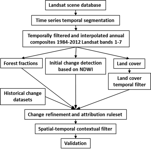
To extract the desired information accurately required numerous processing steps and integration of several data sources. Landsat time series analysis was used to determine change, change rates, land cover, and forest fractions. Change types were assessed using an in depth expert ruleset that combined the results of the Landsat analysis with additional disturbance datasets available for the region regarding fire and anthropogenic impacts. Figure 1 presents an overview with details provided in the following sections.

Figure 1. Overview outlining the key processing steps and datasets used in the analysis.

Landsat processing

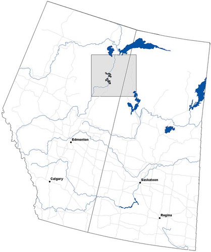
All July and August Landsat 5 and 7 scenes from 1985 to 2012 covering the area of interest shown in Figure 2 were acquired from the United States Geological Survey (USGS) archive. Processing into a standard projection, radiometric calibration, and scene identification (cloud, cloud shadow, water, and snow) were performed using the Moderate Resolution Time Series Data Management and Analysis System developed at the Canada Centre for Remote Sensing (Latifovic et al. 2015). In total, 608 scenes were used. The Lambert conformal conic projection was used based on the GRS-1980 spheroid, latitude of origin 0°, central meridian of −95°, and standard parallels of 49° and 77°. The time series extends only until 2012, due to the loss of Landsat 5 and scan line corrector (SLC) failure of Landsat 7, which greatly limits quality observations post 2012. Extending the time series with Landsat 8 is possible, but the requirement to cross-calibrate with the previous Landsat sensors was beyond the scope of the analysis undertaken here.

Figure 2. Area of interest shown in grey.

Ancillary data

Existing change datasets in vector format characterizing fire and anthropogenic disturbances covering Alberta were used, as these are quality datasets developed through substantial manual effort and/or quality control. These or other similar datasets are available that cover the boreal forest of Canada and thus the methodology is scalable to the national extent, although with associated changes in accuracy. Further, these data provide a significant opportunity to greatly enhance the retrieval of detailed historical change information not easily achieved otherwise.

Anthropogenic disturbances were available from the Alberta Biodiversity Monitoring Institute Human Footprint data (ABMI_HF) containing seismic lines, well points, drainage ponds, forest harvest polygons, etc. covering Alberta up to 2010 in vector format. The vectors in some cases identified the location but did not delineate the feature correctly. For example, well-sites were represented as a standard square that did not match the actual ground footprint. The timing of change events was not provided in the dataset and needed to be derived. Fire polygons were acquired from the National Canadian Large Fire Database (NCLFD). These data provide a generalized outline of the fire, but small unburnt islands may not be removed. Other vector data such as the surface mining footprint was acquired from Global Forest Watch for the years 1992, 2002, and 2008. To derive a complete history of the surface mining these layers were manually modified between years based on visual interpretation of Landsat data for each year. Each of these layers was provided in vector format and was converted to a 30-m raster for use in the analysis. However, to ensure all features in the ABMI_HF data were retained at the 30-m spatial resolution it was first converted to a 5-m raster and then upscaled to 30 m where the majority disturbance was selected for the output. Thus, if only one pixel was flagged as change in the ABMI_HF 5-m raster, it was maintained in the upscaled version. Rasterizing directly to 30 m would not maintain these small disturbance features.

Time-series segmentation

The time-series segmentation approach fits a series of linear-piecewise segments to the data as a form of generalization or temporal smoothing (Kennedy, Yang, and Cohen 2010). These segments can be used to identify rates of change and the change event duration such as abrupt (ideally ≤1 year) or gradual (>1 year). In this implementation, the methodology is adapted from the Landsat scene-based approach made available by Kennedy et al. (2013) to a pixel-based approach. In the scene-based method, best quality scenes are selected for a given Landsat path and row. This is effective in the United States where there are much more scenes collected than elsewhere in world (Kovalskyy and Roy 2013). In Canada, fewer scenes are collected per path–row combination, but there is greater overlap between scenes. Efficiently incorporating the overlap observations can compensate for the reduced scene collection. Scene overlap increases from the equator to the north. For the AOS adjacent, scene overlap is ~40%, in Canada’s far north it reaches ~84%, and at the border with the United States scene overlap is ~30%. Thus, in Canada, a pixel-based approach provides sufficiently more observations than a scene-based does and our implementation of the time-series segmentation algorithm was designed for this aspect.

The methodology was applied to the normalized difference wetness index (NDWI = (B4 − B5)/(B4 + B5), B4, and B5 refer to the Landsat band designations) time series for each pixel in the study area. It is important to note that a pixel-based approach potentially increases the amount of atmosphere and target variability in the time series that needs to be accounted for. To achieve effective results significant preprocessing was implemented in an automated manner and included (1) post-seasonal cloud screening, (2) robust averaging of multiple observations for a given year, (3) optimization of temporal segmentation breakpoints, and (4) trend generalization. Post-seasonal cloud screening involved analysis of the time series for a pixel to identify and remove outliers likely associated with clouds or cloud shadows. It was based on the z-score deviation of the residuals from a Lowess fit to the time series and the original observations. The Lowess fit used a first-degree model and a window size of ±2 years. Observations with an absolute z-score greater than 1.64 (90% confidence) were removed. In the second step, the robust average of multiple observations in a given year was calculated by computing the median and median absolute deviation (MAD), where observations with greater than ±1.64 MAD from the median were removed, and the mean taken of the remaining values (Huber and Ronchetti 2009). Again, the 1.64 threshold was used as a 90% confidence for an assumed normal distribution. To determine the number of breakpoints in the time series the change in the mean absolute fit error (MAE) for 4–7 breakpoints was determined and the largest difference selected for the optimal if its ratio to the previous MAE fit was greater than a factor of 1.25. These thresholds and breakpoint ranges were empirically derived by testing numerous samples for different land-cover types and changes throughout the study area. The additional generalization step was used to improve the change rate/duration estimate by merging temporal segments with a similar slope (±0.15 NDWI/year) and direction (negative or positive). The generalization result was maintained separately from the initial segmentation results and only used in the change-type determination.

The breakpoints identified from the NDWI temporal segmentation were used to produce similarly smoothed time series for all Landsat bands as discussed in Kennedy et al. (2013). Linear segments were fit between breakpoints using each Landsat band as the data source. Missing observations were estimated from the piecewise fit. These smoothed data were used in subsequent estimation of land cover and forest fractions.

Land-cover and -disturbance classification

A sample of land cover was derived from interpretation of available GeoEye (0.5-m pan sharpened), RapidEye (5 m), and Ikonos (3 m) high-resolution imagery and ground truth points. Basic land-cover types were sought and included: (1) needleleaf forest, (2) open needleleaf forest and treed wetland, (3) mixed forest, (4) deciduous forest, (5) shrub, (6) low vegetation, (7) bare, (8) non-tree wetland, and (9) water. In addition, a sample of disturbance classes was developed and included: (1) harvest, (2) fire, (3) insect damage, (4) haze, (5) flood, and (6) no disturbance. Data were used to train a decision tree classifier developed in SEE5 (Quinlan 1993) using 40 bootstrap iterations and fuzzy-decision thresholds. SEE5 has been shown to be an effective classifier for land-cover mapping (Friedl et al. 2002; Latifovic et al. 2012), change detection (Pouliot et al. 2009), and sea-ice mapping (Kim et al. 2015). The classifier was applied to the temporally smoothed Landsat time series to provide an estimate of land-cover or -disturbance type for each year. The class memberships were retained for use in the change-type determination. The purpose of the land-cover classification was twofold. The first was to provide “from-to” land-cover change information. The second was to generate a potentially more stable land-cover time series with the piecewise temporal-segmentation approach in a more efficient manner than the more common change-detection and change-update approach outlined in Pouliot et al. (2012).

Land cover segment-based temporal filter

The temporal-segmentation results provide a unique opportunity to enhance land-cover time series consistency as segments, not detected as change, should have the same land cover in all years. Based on this principle, we developed a segment-specific time series filter where, for segments not detected as change, the mode of the land cover in all years of the segment was taken for segments greater than 8 years, the segment was split and the mode taken for each split. Additional splits were made such that the mode was not taken for segments consisting of less than 4 years and not more than 8 years. The purpose of the splitting was to account for missed changes where land cover may have undergone a subtle transition to another class. For segments detected as gradual change (either positive or negative), the mode was taken every 5 years using a moving window. No filtering was applied to segments detected as abrupt change.

Forest-fraction modeling

Forest-fraction data were used to represent a measure of change severity. For a temporal segment identified as change, the difference in forest fraction for each year of the segment was calculated as measure of the change severity. Fractional data were modeled as described in Pouliot, Parkinson, and Latifovic (2015) using RandomForest (Breiman 2001), Landsat observations, and reference fractions derived from classified high-spatial resolution GeoEye imagery (2 m). Fractional models were applied to the temporally smoothed data produced in this study. Fraction accuracy was estimated to be around 15% on average in Pouliot, Parkinson, and Latifovic (2015).

Human-footprint harvest timing

The temporally smoothed time series was used to estimate the year of occurrence for the ABMI_HF harvest polygons. This information was not included in the ABMI_HF layer. In the first step, the time series for a harvest pixel was extracted and the points for which a change threshold was met were extracted. The membership for the bare class was examined to determine the most likely year for the forest harvest. In some cases, no clear year could be identified and a fill value of 1 was used. In the second step, a mode filter was passed over the results, where only values greater than 1 and NDWI values within ±10% of the central value were considered within a 9 × 9 moving window. A few remaining errors were found in some places and were manually corrected.

Change-type ruleset

Expert rules were developed to classify changes as specified in Table 1. Rules were based on the duration of the change event, post-disturbance spectral response, land cover or disturbance class/membership before or after change, or association with ancillary disturbance data. In this region, classification of fire, harvest, or surface mining was difficult as they are all abrupt changes and post-disturbance spectral responses can be similar. For example, fires in lower density forest with sand rock ground cover can have a similar spectral response to that of a forest harvest. The integration of the ancillary change datasets resolved this problem. In total, 15 different rulesets were developed to assign changes to classes. For the ruleset implementation, segments were detected as change if the forest fraction change was greater than 25% and the NDWI changed by a threshold of ±0.15. After applying the ruleset, changes that were not identified as one of the specific change types listed in Table 1, were not considered change. This helped to reduce commission errors. Further, to make the ruleset more robust the definition of abrupt change was altered to ≤2 years to account for error in the temporal segmentation, which due to noise and sparse observations in some cases caused abrupt changes to be represented by more than a single year.

Table 1. Change classes and rulesets used for change type classification.

Class	Ruleset
Forest harvest	Abrupt change segment associated with ABMI_HF harvest polygon detected year and post-disturbance spectral response >50% bare membership and post-disturbance land cover was not needleleaf, broadleaf, or mixed forest. Pre-disturbance land cover was either needleleaf, broadleaf, or mixed forest
Fire	(1) Abrupt change segment associated with NCLFD fire polygon and post-disturbance spectral response with >50% fire membership and post-disturbance land cover was not needleleaf, broadleaf, or mixed forest. (2) Abrupt change segment with post-disturbance spectral response >80% fire membership and post-disturbance land cover was not needleleaf, broadleaf, or mixed forest. This is a conservative rule that accounts for fires missed in the NCLFD
Insect damage	Gradual change segment and insect-damage membership > bare, flood, or fire memberships and pre-disturbance forest needleleaf, broadleaf, or mixed-forest membership was >70%
Flooding	Segments where post-disturbance water membership was greater than 60% for more than 2-years post-disturbance
Regeneration	Temporal segments that increased their forest fraction by 20% over at least 3 years and the final forest fraction was greater than 20% following disturbance. To account for disturbances prior to 1985, this rule was applied to the first segment in the time series
Surface mining	Segments that had a harvest-spectral membership post-disturbance >50% and were associated with the crude mining footprint mask for the year
Abrupt disturbance without regeneration	Changes that occurred rapidly (≤2 years), were not followed by regeneration as per criteria for regeneration, and were not previously classified to a change type. This class was commonly associated with mining or exploration activities such as roads, pipelines, well pads, etc.
Gradual disturbance without regeneration	Changes that occurred gradually (>2 years), were not followed by regeneration as per criteria for regeneration, and were not previously classified to a change type
Abrupt disturbance with regeneration	Changes that occurred rapidly (≤2 years) with regeneration as per criteria for regeneration, and were not previously classified to a change type
Gradual disturbance with regeneration	Changes that occurred gradually (>2 years) with regeneration as per criteria for regeneration, and were not previously classified to a change type
Spectral variability likely associated with wetlands	Areas of change where the pixel was classified as wetland more than four times in the time series
Unclassified	Changes with small magnitude that were not assigned to another class. This was largely due to commission error and not included as change
Haze	Segments identified as change with a haze membership greater than 80% and not associated with a harvest or fire disturbance. These segments were not considered change

Contextual filter for change timing and type attribution

To reduce pixel-scale noise in the final results a contextual filter was developed where the change class was assessed within a 3 × 3 × 5 moving window. The 3 × 3 plane was the spatial dimension for a given year while the 3rd dimension represented years. It consisted of ±2 years from the year being processed. Within the 3 × 3 × 5 subset data, the majority class was assigned if it was non-zero. The temporal sequence of change for the central pixel was also checked for odd-change occurrences such as fire-flood or mine-fire etc. These were flagged and checked. Only 40 pixel were found of this type. For the change year, the majority-maximum and majority-minimum year were determined within the sample window for pixels with the same change class and used as the temporal range for the pixel being processed. This removed speckle-type errors throughout the results altering the label for less than 5% of the total change area.

Validation

To generate an independent sample for validation in a cost-effect manner a stratified random sample was generated within the domain of available high-spatial resolution (≤10 m) imagery. High-resolution data covered approximately 60% of the study area. For each change type 10 samples were selected for two periods between 1985–1999 and 2000–2012. Thus, for the 11 change types evaluated there were 10 × 2 × 11 = 220 samples. In addition, 40 no-change samples were randomly selected. Sample points were interpreted using the high-spatial resolution data and Landsat time series to determine the most likely change cause, start and end timing, and land cover before and after the change. Thus, the total number of samples for land cover was 520. The following comparison statistics were generated: a basic change/no-change error matrix, change-type error matrix, change-timing error statistics, and a land-cover error matrix.

Results and discussion

Temporal-segmentation performance

Example results for the time-series segmentation of a single pixel are shown in Figure 3A–D. Figure 3A shows the cloud-and shadow-screened Landsat observations for each year. The blue line represents the average value in each year. This time series shows a forest harvest that occurred in 1989 and a fire in 2011 as depicted in the subset Landsat images. The temporal-segmentation results are shown in red in Figure 3B. It has effectively captured the forest harvest as a 1-year change event followed by a period of slow regeneration. The fire, however, in 2011 was broken into two segments. The generalization procedure that merged temporal segments based on slope similarity corrected this representing it as one segment when used in the change-type ruleset. An example of gradual change related to insect damage is shown in Figure 3C–D. The change appears to start in 2000 and ends in 2010. The temporal segmentation performed well, except for the small increasing segment captured between 2003 and 2004. Again the generalization procedure corrected this error when examining the duration of the change event in the change-type classification ruleset.

Figure 3. Example time series for harvesting in 1989 and fire in 2011 (A–B) and insect damage (C–D). Cloud- and shadow-screened time series are shown as asterisks. Blue line represents average value in each year. Sub-trend time series results (red line) from the average values shown as the black line.

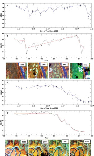
Numerous other example cases were extracted and revealed very good performance for single-change events that did not occur at the start (1984) or end (2012) of the time series. Multiple-change events that occurred close in time were sometimes confused as a single-change event. Some abrupt changes associated with mining close to the start of the time series were captured as gradual events (3–4 year) due in part to edge effects. For example, pre-mining exploration, hydrological change associated with nearby mining, and mine-initiation activities often cause vegetation conditions to decline before mining begins. This caused the time series to have an initial slow decline followed by a more rapid deterioration due to the direct vegetation removal phase of the mine development. Capturing these as separate time-series events is difficult due to noise and limited temporal sampling of Landsat. This only affected the timing of the change event. The change magnitude was still representative of the disturbance; it was just spread over several years. Edge effects also resulted from the Landsat 7 SLC-error (missing lines in Landsat 7 data since 2003) which made it difficult to detect some changes in 2012, as actual changes which were confused with or seen as time-series noise in some of the processing steps.

Validation

The basic change/no-change confusion matrix was derived to reveal performance relative to other change detection studies (Table 2). The accuracy estimate of 89% is within the range of other large-area forest change studies (Zhan et al. 2002; Fraser et al. 2005; Pouliot et al. 2009; Xian, Homer, and Fry 2009; Potapov, Turubanova, and Hansen 2011; Guindon et al. 2014). In this analysis, the small size of the changes desired to be detected resulted in a general bias toward commission error. Most of the commission error detected in Table 2 was due to spectral variance associated with inter-annual hydrology that was confused as forest change. In this region, the more hydric conditions lead to changes in the underlying soil spectral characteristics that were easily observed by the Landsat sensors due to the lower density tree canopies relative to other parts of the boreal forest in Canada. Of the 20 commission errors, 18 were associated with hydrological variability. Removing these errors increased the overall accuracy to 95%. Omission error was much lower and was mostly associated with small disturbances such as well sites or roads that covered less than 2–3 pixels.

Table 2. Change/no-change error matrix.

	Reference
	Change	No-change
Change	193	20
No-change	9	37
Overall accuracy %		89

The error matrix for specific-change types is given in Table 3. Table 4 shows the mean, standard deviation, 90th percentile, and max error for the change regarding the timing of the change start and end estimate. Overall accuracy for the change-type classification was 82%. Abrupt changes such as fires, harvesting, and surface mining had good classification accuracies and were generally within ±1 year of the change timing estimates. The accuracy for flooding was also very good, but visual examination of the results suggests that flooding had lower detection rates than what was estimated in Table 3. It had the highest error rate regarding the timing of the detected change for the abrupt change types. Most of the flooding-related change occurred in the surface-mine area where there were often initial exploration/preparation activities, land clearing, and then flooding. This sequence was often captured as a multi-year event instead of separate change events. The insect-damage class was classified with a user’s accuracy of 75%. The main sources of confusion were with fires and wetland variability. The lowest accuracies were found for the generic gradual change classes and again confusion was largely associated with wetland dynamics for both classes. These classes only covered a small portion of the study area so it was not considered a significant factor on accuracy. The abrupt change without regeneration class achieved a user’s accuracy of 81% and was largely caused by industrial development-related disturbances such as well pads, roads, pipelines, etc. that occurred outside the main surface mining developments. This class could be considered as deforestation. The regeneration class was not assessed for timing because interpretation of subtle regrowth in many cases could not be achieved with reasonable confidence.

Table 3. Change type error matrix.

		Reference
		1	2	3	4	5	6	7	8	9	10	11	12
Forest harvest	1	20	0	0	0	0	0	0	0	0	0	0	0
Forest fire	2	0	20	0	0	0	0	0	0	0	0	0	0
Insect damage	3	0	2	15	0	0	0	0	0	0	0	3	0
Flooding	4	0	0	0	20	0	0	0	0	0	0	0	0
Forest regeneration	5	0	0	0	0	20	0	0	0	0	0	0	1
Surface mining	6	0	0	0	0	0	20	0	0	0	0	0	0
Abrupt dist. no regen.	7	1	0	0	0	0	2	15	0	0	0	1	0
Gradual dist. no regen.	8	0	0	0	0	0	0	2	12	0	0	7	1
Abrupt dist. regen.	9	4	0	0	0	0	0	0	1	11	0	2	2
Gradual dist. regen.	10	1	0	1	0	0	0	0	0	0	7	9	2
Wetland variability	11	0	0	0	0	0	0	1	0	0	0	18	0
No Change	12	0	0	1	0	3	0	0	0	0	0	0	35
Producer’s accuracy %		77	91	88	100	87	91	83	92	100	100	45	85
User’s accuracy %		100	100	75	100	95	100	79	55	55	35	95	90
Ave. prod. and user’s %		88	95	82	100	91	95	81	73	78	68	70	88
Overall accuracy %		82

Table 4. Change error timing estimates by change type.

	Error start year					Error end year
Change type	Abs mean Std. Dev. 90%ile			Max	Abs mean	Dev. 90%ile		Max
Forest harvest	0.30	0.92	1	4	0.2	0.89	0	4
Fire	0.10	0.31	0	1	0.1	0.22	0	1
Insect damage	0.25	0.64	1	2	1.1	1.74	3	6
Flooding	3.00	2.87	7	9	1.9	1.77	3	6
Surface mining	1.05	1.76	4	6	0.5	0.61	1	2
Abrupt dist. no regen.	0.11	0.32	1	1	0.0	0.00	0	0
Gradual dist. no regen.	0.32	0.89	1	3	0.2	0.40	1	1
Abrupt dist. regen.	0.10	0.31	0	1	0.2	0.41	1	1
Gradual dist. regen.	0.15	0.49	0	2	0.4	1.35	1	6
Wetland variability	0.00	0.00	0	0	0.1	0.23	0	1

*Regenaration and haze classes were not assessed as interperation in the available reference data was insufficient.

The land-cover data was developed to aid in the change-type classification and was not designed to be a highly accurate land-cover time series as limited resources were available for its development. Regardless it does provide useful information on the land-surface changes over time. Results are shown in Table 5 and reveal that an overall accuracy of 69% was achieved. Sampling the land cover before and after the change biased the accuracy to a slightly lower value as errors in change timing led to land-cover misclassification. Also the water class was under-sampled partially leading to the low accuracy observed. Confusion between shrub, low vegetation, and bare was a significant source of error and for many applications these classes could be merged to improve accuracy. For a five class legend of needleleaf forest, mixed forest, broadleaf forest, shrub, and water an overall accuracy of 80% was achieved.

Table 5. Land-cover error matrix.

		Reference
		1	2	3	4	5	6	7	8	10
Needleleaf high density	1	53	4	1	0	2	6	1	1	0
Needleleaf low density	2	11	56	0	2	10	8	4	4	3
Mixed forest	3	1	1	13	0	1	4	0	1	0
Broadleaf	4	2	5	3	41	9	0	1	0	0
Shrub	5	1	2	3	3	78	20	6	0	0
Low vegetation cover	6	2	4	0	0	1	39	4	0	0
Barren	7	4	4	1	0	0	3	38	2	3
Wetland	8	0	0	0	1	6	2	0	16	0
Water	10	3	1	0	0	1	0	1	0	22
Producer’s accuracy %		69	73	62	87	72	48	69	67	79
User’s accuracy %		78	57	62	67	69	78	69	64	79
Ave. prod. and user’s %		73	65	62	77	71	63	69	65	79
Overall accuracy %		69

Spatial and temporal dynamics of land-cover change in AOS

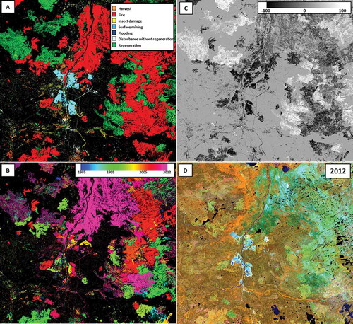
Summary results showing the spatial distribution of changes are shown in Figure 4; (A) change type for the most recent disturbance or regeneration if no disturbance occurred, (B) change year for the change event given in A, (C) change severity which represents the net change over the time series, and (D) Landsat composite for year 2012 for comparison. Results show that the dominant disturbance was fire with large recent fires occurring in the northeast. Older pre-1985 fires can be seen as regenerating throughout the region, particularly in the northwest. Mining is the second largest disturbance agent. Insect damage resulting in tree mortality largely appeared to affect needleleaf forests and occurred dominantly in the southeast, often associated with rivers or other open areas. Defoliation of aspen was observed in field campaigns and is consistent with previous aspen defoliator surveys. However, due to rapid recover of the canopy aspen defoliation was not captured in this analysis.

Figure 4. Summary of the change types for most recent change (A), year of most recent change (B), change severity of most recent change (C), and Landsat composite for 2012 for comparison (D).

Gradual changes such as regeneration or insect damage are represented over a number of years in the time series and thus the change-type flag was repeated over several years. The forest-fraction data were more representative in this case. Figure 5A–B shows the time series of change type by pixel count converted to hectares and by the sum of forest-fraction change for each change type. From Figure 5 regeneration is seen as the most significant change factor due to several large pre-1985 fires regenerating over the period. It however, slows due to forest re-establishment of these fires and an increase in forest disturbance over time. Fire is the major source of negative change. As expected, surface mining is increasing as is disturbance without regeneration which is associated with mine development and exploration. Insect damage is also increasing and appears as a large source of disturbance in the region. Little harvesting has taken place on a relative basis.

Figure 5. Trends in change type. (A) Pixel count converted to hectares and (B) Sum of forest fraction change by change type. Note the scaling for fire and the secondary axis used for regeneration to enhance interpretability. In (B), all disturbances have been multiplied by −1 and actually represent a negative forest fraction change.

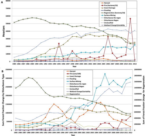
It is interesting to compare the pixel-based and change-fraction sum results between Figure 5A and B. If all disturbances were of equal severity then these two graphs should be the same. Clearly this is not the case. In the change-fraction sum results, severe disturbances such as surface mining and harvesting have much greater impact than the pixel-based results would suggest, due to their greater change severity. In these results, the effect of harvesting, insect damage, and surface mining are more similar which is contradictory to the pixel-sum results. So although more area is affected by insect damage its net effect is similar to that of harvesting and less than that of surface mining because it is not as severe of a disturbance. The “disturbance with regeneration” class decreases through time and is in part a temporal artifact as recent disturbances cannot be assessed for regeneration with the ruleset developed.

The amount of insect damage was an unforeseen result. It is important because it presents an impact on the ecosystem goods and services in the region that are possibly under stress due to other activities such as fire, harvesting, and mining. More research is required to evaluate if the level of insect damage observed is outside of historical ranges and to assess the potential role of industrial development.

The temporal trends for the land-cover results were also assessed and are summarized in Figure 6A. It shows that open needleleaf and low-vegetation cover were the two classes with the biggest decrease over time. The decrease in open needleleaf was due to disturbance, whereas the change in the low-veetation cover class was due to regeneration. In 1984, several pre-1984 fires had caused much of the landscape to be in a disturbed-forest state. The bare class increased over time due to mining and mining-related infrastructure development. Shrub increase was due to older fires and harvest disturbance that regenerated from bare/low vegetation cover to shrub. Water, broadleaf, wetland, and needleleaf classes were relatively stable. It is important to note that this is not a strongly quality controlled land-cover product. There is considerable interclass shifting along class boarders in the maps between years that potentially could hide some trends. The temporal-filtered version of the land cover was more stable (Figure 6B), but the filtering lead to some abrupt changes in the time series due to the generalization. For example, the decrease in open needleleaf between 1997 and 1998 was due to a large number of 1998 fires. The rapid increase in mixed forest between 1997 and 1998 was due to regeneration and the temporal filter, where the mode was taken from 1997 to 2004 in the northwestern portion of the study area.

Figure 6. Trends in land cover for pixel count converted to hectares based on the original land cover (A) and the temporally filtered (B).

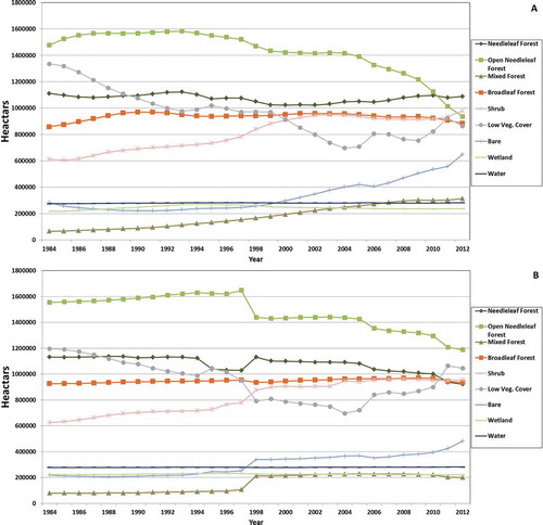
In the current version of the product, regeneration may appear to be underestimated. This was the result of using a 20% forest fraction as the threshold to define regeneration and in a relative sense the short duration of the time series of 29 years. Generally, it takes more than 20 years to redevelop to a boreal forest like condition and the time series is too short to observe this in many cases. Regeneration from bare to herb to shrub is taking place that this product does not capture in its current form. Refined calibration or definitions of regeneration could change this aspect.

A limitation of the method developed here, particularly for the AOS, is that small linear features are poorly or not detected. A 3-m wide cut line through a Landsat pixel accounts for only (3 m × 30 m/30 m²) 10% of the pixel area. This is a small area and depends on the spectral contrast between the overstory and understory. For example, a cut line through a deciduous forest is less distinct than through a needleleaf forest, because the thicker shrub-herb understory can have a spectral response similar to the deciduous-tree canopy. In dense needleleaf forests, the acidic needles keep the understory to a minimum and thus the post-disturbance spectral response tends to contrast well with the needleleaf canopy. In a recent study by Pasher, Seed, and Duffe (2013), omission error as high as 60% was found for linear-feature detection based on manual interpretation of Landsat.

Results for a more automated approach to linear-feature detection in Alberta based on temporal analysis of Landsat also did not suggest a strong potential for detection (Zhaohua et al. 2014). Although detection accuracy with Landsat may be low, the total area of linear-feature disturbance is also low reducing the need for detection in analysis that does not depend strongly on the spatial pattern of the change.

The methods tested here are extendable to the national scale as suitable databases have been developed in Canada. The fire database used in this study is national and covers a sufficient historical range, although accuracy between regions is variable due to different mapping methods (NCLFD). For more recent fires from 2005 onward, a more standardized approach has been used (Stinson et al. 2011; NBAC 2016). The database described in Pasher, Seed, and Duffe (2013) would provide linear features and other polygon-type disturbances covering the Canadian boreal forest, although accuracy would be lower than the ABMI_HF used in this analysis. The ABMI_HF was derived from higher resolution imagery than the Landsat data used in Pasher, Seed, and Duffe (2013). An important consideration is that the occurrence of linear- and other small-change features do not occur in such high frequency as that found in the AOS region. Thus, change and attribution accuracy could possibly be more accurate than the validation undertaken here would suggest at the national scale. Another key point is that the method developed may not be needed at the national scale, but can be employed in important study areas where more detailed change information is needed. For such studies, the required ancillary-disturbances datasets can be developed from high-spatial resolution or semi-manual methods.

Conclusions

Landsat time series provides significant capacity to generate detailed information on the spatial–temporal development of change. Here, we show a complete example application for the AOS. Much of this capacity can be automated, but still to achieve sufficient results manual intervention was required and is a typical practice in the generation of quality products. The integration of the fire- and AMBI_HF-disturbance datasets provided the capacity to achieve effective change type attribution and is extendable to the national scale or can be redeveloped for specific study sites. Such an approach is favorable as it utilizes high-quality datasets for which significant investments have already been made. This dataset serves as prototype for testing landscape-processes models were sensitivity to land-cover change is expected to impact model results.

Acknowledgements

This research was partly support by the Canadian Space Agency, Government Related Initiatives Program IMOU number 13MOA41001, Enabling Responsible Resources Development through Earth Observation. It was completed as part of a collaboration with the Canadian Forest Service lead by Dr. Werner Kurz and Dr. Cindy Shaw.

Disclosure statement

No potential conflict of interest was reported by the authors.

References

- Breiman, L. 2001. “Random Forests. Machine Learning”, Online Report. https://www.stat.berkeley.edu/~breiman/randomforest2001.pdf
- Bucha, T., and H. Stibig. 2008. “Analysis of MODIS Imagery for Detection of Clear Cuts in the Boreal Forest in North-West Russia.” Remote Sensing of Environment 112: 2416–2429. doi:10.1016/j.rse.2007.11.008.
- Chhabra, A., H. Geist, R. A. Houghton, H. Haberl, A. K. Braimoh, P. L. Vlek, J. Patz, et al. 2006. “Multiple Impacts of Land-Use/Cover Change.” In Land-Use and Land-Cover Change Local Processes and Global Impacts, edited by E. F. Lambin and H. Geist, 71–116, Berlin Heidelberg: Springer-Verlag.
- Fraser, R. H., A. Abuelgasim, and R. Latifovic. 2005. “A Method for Detecting Large-Scale Forest Cover Change Using Coarse Spatial Resolution Imagery.” Remote Sensing of Environment 95: 414–427. doi:10.1016/j.rse.2004.12.014.
- Fraser, R. H., I. Olthof, and D. Pouliot. 2009. “Monitoring Land Cover Change and Ecological Integrity in Canada’s National Parks.” Remote Sensing of Environment 113: 1397–1409. doi:10.1016/j.rse.2008.06.019.
- Friedl, M. A., D. K. McIver, J. C. F. Hodges, X. Y. Zhang, D. Muchoney, A. H. Strahler, C. E. Woodcock, et al. 2002. “Global Land Cover Mapping from MODIS: Algorithms and Early Results.” Remote Sensing of Environment 83: 287–302. doi:10.1016/S0034-4257(02)00078-0.
- Fry, J. A., G. Xian, S. Jin, J. A. Dewitz, C. G. Homer, L. Yang, C. A. Barnes, N. D. Herold, and J. D. Wickham. 2011. “Completion of the 2006 National Land Cover Database for the Conterminous United States.” Photogrammetric Engineering and Remote Sensing 77: 858–864.
- Gillanders, S., N. C. Coops, N. Goodwin, and M. Wulder. 2008. “Application of Landsat Satellite Imagery to Monitor Land Cover Changes at the Athabasca Oil Sands, Alberta, Canada.” Canadian Geographer 52 (4): 466–485. doi:10.1111/j.1541-0064.2008.00225.x.
- Guindon, L., P. Y. Bernier, A. Beaudoin, D. Pouliot, P. Villemaire, R. J. Hall, R. Latifovic, and R. St-Amant. 2014. “Annual Mapping of Large Forest Disturbances across Canada’s Forests Using 250 M MODIS Imagery from 2000 to 2011.” Canadian Journal of Forest Research 44: 1545–1554. doi:10.1139/cjfr-2014-0229.
- Hall, R., R. Skakun, and E. Arsenault. 2007. “Remotely Sensed Data in the Mapping of Insect Defoliation.” In Understanding Forest Disturbance and Spatial Pattern: Remote Sensing and GIS Approaches, edited by M. Wulder and S. Franklin, Chap. 4, 85–111, 253 pp. FL, USA: Taylor & Francis Group.
- Hansen, M., D. Roy, E. Lindquist, B. Adusei, C. O. Justice, and A. Altstatt. 2008. “A Method for Integrating MODIS and Landsat Data for Systematic Monitoring of Forest Cover and Change in the Congo Basin.” Remote Sensing of Environment 112: 2495–2513. doi:10.1016/j.rse.2007.11.012.
- Huang, C., S. Goward, J. Masek, N. Thomas, Z. Zhu, and J. Vogelmann. 2010. “An Automated Approach for Reconstructing Recent Forest Disturbance History Using Dense Landsat Time Series Stacks.” Remote Sensing of Environment 114: 183–198. doi:10.1016/j.rse.2009.08.017.
- Huber, P., and E. Ronchetti. 2009. Robust Statistics. 2nd ed. New York: John Wiley and Sons.
- Keely, J. E. 2009. “Fire Intensity, Fire Severity and Burn Severity: A Brief Review and Suggested Usage.” International Journal of Wildland Fire 18: 116–126. doi:10.1071/WF07049.
- Kennedy, R., J. Braaten, Z. Yang, P. Nelson, and M. Duane. 2013. “LandTrendr Version 3.0, Users Guide, Version 0.1”. http://landtrendr.forestry.oregonstate.edu/content/downloads.
- Kennedy, R. E., Z. Yang, and W. B. Cohen. 2010. “Detecting Trends in Forest Disturbance and Recovery Using Yearly Landsat Time Series: 1. Landtrendr—Temporal Segmentation Algorithms”.” Remote Sensing of Environment 114: 2897–2910. doi:10.1016/j.rse.2010.07.008.
- Kim, M., I. Jungho, H. Hyangsun, K. Jinwoo, L. Sanggyun, S. Minso, and K. Hyun-Cheol. 2015. “Landfast Sea Ice Monitoring Using Multisensor Fusion in the Antarctic.” GIScience and Remote Sensing 52: 239–256. doi:10.1080/15481603.2015.1026050.
- Kovalskyy, V., and D. P. Roy. 2013. “The Global Availability of Landsat 5 TM and Landsat 7 ETM+ Land Surface Observations and Implications for Global 30m Landsat Data Product Generation.” Remote Sensing of Environment 130: 280–293. doi:10.1016/j.rse.2012.12.003.
- Lambert, J., C. Drenou, J. Denux, G. Balent, and V. Cheret. 2013. “Monitoring Forest Decline through Remote Sensing Time Series Analysis.” GIScience and Remote Sensing 50: 437–457.
- Latifovic, R., K. Fytas, J. Chen, and J. Paraszczak. 2005. “Assessing Land Cover Change Resulting from Large Surface Mining Development.” International Journal of Applied Earth Observation and Geoinformation 7: 29–48. doi:10.1016/j.jag.2004.11.003.
- Latifovic, R., C. Homer, R. Ressl, D. Pouliot, S. Hossian, R. Colditz, I. Olthof, C. Giri, and A. Victoria. 2012. “North American Land Change Monitoring System.” In Remote Sensing of Land Use and Land Cover, edited by C. Giri, 303–324. Boca Raton, FL: Taylor and Francis Group.
- Latifovic, R., and D. Pouliot. 2014. “Monitoring Cumulative Long-Term Vegetation Changes over the Athabasca Oil Sands Region.” IEEE Journal of Selected Topics in Applied Earth Observations and Remote Sensing 7: 3380–3392. doi:10.1109/JSTARS.2014.2321058.
- Latifovic, R., D. Pouliot, L. Sun, J. Schwarz, and W. Parkinson. 2015. “Moderate Resolution Time Series Data Management and Analysis: Automated Large Area Mosaicking and Quality”. Canada Center for Mapping and Earth Observation, Geomatics Canada Open File. doi:10.4095/296204.
- Latifovic, R., and D. A. Pouliot. 2005. “Multi-Temporal Land Cover Mapping for Canada: Methodology and Products.” Canadian Journal of Remote Sensing 31: 347–363. doi:10.5589/m05-019.
- Manqi, L., J. Im, and C. Beier. 2013. “Machine Learning Approaches for Forest Classification and Change Analysis Using Multi-Temporal Landsat TM Images over Huntington Wildlife Forest.” GIScience and Remote Sensing 50: 361–384.
- NBAC (National Burned Area Composite). 2016. “Fire Monitoring and Reporting Tool.” Accessed April 2015. http://www.nrcan.gc.ca/forests/fire-insects-disturbances/fire/13159
- Pasher, J., E. Seed, and J. Duffe. 2013. “Development of Boreal Ecosystem Anthropogenic Disturbance Layers for Canada Based on 2008 to 2010 Landsat Imagery.” Canadian Journal of Remote Sensing 39: 42–58. doi:10.5589/m13-007.
- Potapov, P., M. Hansen, S. Stehman, T. Loveland, and K. Pittman. 2008. “Combining MODIS and Landsat Imagery to Estimate and Map Boreal Forest Cover Loss.” Remote Sensing of Environment 112: 3708–3719. doi:10.1016/j.rse.2008.05.006.
- Potapov, P., S. Turubanova, and M. C. Hansen. 2011. “Regional-Scale Boreal Forest Cover and Change Mapping Using Landsat Data Composites for European Russia.” Remote Sensing of Environment 115: 548–561. doi:10.1016/j.rse.2010.10.001.
- Pouliot, D., R. Latifovic, R. Fernandes, and I. Olthof. 2009. “Evaluation of Annual Forest Disturbance Monitoring Using Decision Trees and MODIS 250m Data.” Remote Sensing of Environment 113: 1749–1759. doi:10.1016/j.rse.2009.04.008.
- Pouliot, D., R. Latifovic, I. Olthof, and R. Fraser. 2012. “Supervised Classification Approaches for the Development of Land Cover Time Series.” In Remote Sensing of Land Use and Land Cover, edited by C. Giri, 177–190. Boca Raton, FL: Taylor and Francis Group.
- Pouliot, D., R. Latifovic, N. Zabcic, L. Guindon, and I. Olthof. 2013. “Development and Assessment of a 250 M Spatial Resolution MODIS Annual Land Cover Time Series (2000-2011) for the Forest Region of Canada Derived from Change-Based Updating.” Remote Sensing of Environment 140: 731–743. doi:10.1016/j.rse.2013.10.004.
- Pouliot, D., W. Parkinson, and R. Latifovic. 2015. “Evaluation of Landsat Based Fractional Land Cover Mapping in the Alberta Oil Sands Region”. Canadian Center for Mapping and Earth Observation, Geomatics Canada Open File. doi:10.4095/296802.
- Quinlan, J. R. 1993. C4.5: Programs for Machine Learning. San Francisco, CA: Morgan Kaufmann Publishers. ISBN:1-55860-238-0.
- Ramankutty, N., L. Graumlich, F. Achard, D. Alves, A. Chhabra, R. S. DeFries, J. A. Foley, et al. 2006. “Global Land Cover Change: Recent Progress, Remaining Challenges.” In Land-Use and Land-Cover Change Local Processes and Global Impacts, edited by E. F. Lambin and H. Geist, 9–40, Berlin Heidelberg: Springer-Verlag.
- Stinson, G., W. Kurz, C. Smyth, E. Neilson, C. Dymond, J. Metsaranta, C. Boisvenue, et al. 2011. “An Inventory-Based Analysis of Canada’s Managed Forest Carbon Dynamics, 1990 to 2008.” Global Change Biology 17: 2227–2244. doi:10.1111/gcb.2011.17.issue-6.
- Xian, G., C. Homer, and J. Fry. 2009. “Updating the 2001 National Land Cover Database Land Cover Classification to 2006 Using Landsat Change Detection Methods.” Remote Sensing of Environment 113: 1133–1147. doi:10.1016/j.rse.2009.02.004.
- Zhan, X., R. Sohlberg, J. R. G. Townshend, C. DiMiceli, M. Carroll, J. Eastman, M. Hansen, and R. Dfries. 2002. “Detection of Land Cover Changes Using MODIS 250 M Data.” Remote Sensing of Environment 83: 336–350. doi:10.1016/S0034-4257(02)00081-0.
- Zhaohua, C., B. Jefferies, P. Adlakha, B. Salehi, and D. Power. 2014. “Monitoring Linear Disturbance Footprint Based on Dense Time Series Landsat Imagery.” Canadian Journal of Remote Sensing 40 (5): 348–361. doi:10.1080/07038992.2014.987375.
- Zhu, Z., and C. E. Woodcock. 2014. “Continuous Change Detection and Classification of Land Cover Using All Available Landsat Data.” Remote Sensing of Environment 144: 152–171. doi:10.1016/j.rse.2014.01.011.