GIS-based modeling of a rescaled surface of land development pressure in the Macaronesian islands

Abstract

Land development is one of the major anthropogenic processes shaping environmental sustainability. However, no standard method exists for evaluating this spatial process. This article proposes a method of modeling a spatially explicit representation of land development pressure, resorting to an inverse distance weighting interpolation. The study area encompasses four Macaronesian islands where land development has caused dramatic changes to the landscape: São Miguel, Madeira, Gran Canaria, and Tenerife. The method is demonstrated over 1990–2006, a period marked by a rapid increase in land development which ended with the 2007–2008 financial crisis. First, centroids of land change in/into artificial surfaces were used as a proxy of land development pressure. Second, these centroids were coupled with ancillary sampled points, which took into account a topographic resistance factor representing areas absent of land change. These ancillary points allowed for confinement of the interpolation values while acting as structural information for the rescaling of the interpolation into a higher resolution of a digital elevation model. The results show that the method captured the overall trend and magnitude of artificial land change. Quantifying and identifying the islands’ pattern of land development pressure creates a variable that can play an important role in further modeling of anthropogenic spatial processes.

Keywords:

• land change
• interpolation
• rescaling
• geostatistics
• Macaronesia

1. Introduction

The increased awareness on issues related to environmental sustainability, confronted with intensifying land development, has increased the importance of land-use/land-cover (LULC) change assessment (Wickham, O’Neill, and Jones 2000; Jaimes et al. 2010; Peneva-Reed 2014). There is consensus that land development is one of the major anthropogenic processes shaping environmental sustainability (Jarnagin 2004; Berlanga-Robles and Ruiz-Luna 2011; Cunningham et al. 2015; Abdullahi et al. 2015). In addition, research recognizes the need to identify, quantify, and explain LULC driving forces (Christman et al. 2015). However, no standard method exists for quantifying and evaluating a spatially explicit representation of land development pressure. To support planning and decision-making, one of the key applications of geographical information science relies in geospatial modeling (Estoque and Murayama 2014). In this regard, a modeled surface of land development pressure can play an important role as an explanatory variable, further modeling a multitude of environmental, social, and economic processes. Therefore, this article proposes a geographical information science-based method of mapping land development pressure suitable for application elsewhere.

In the last decades, human-induced landscape changes were profound at a global scale (Foley et al. 2005). These changes have also affected the small and isolated Macaronesian islands of Portugal and Spain. Over the last few decades, fast growing tourism activity has caused dramatic changes to the islands’ landscape. Because of limited land and geographical isolation, the land-change process is magnified in comparison with mainland regions. Moreover, due to the islands’ ecological importance (Fernández-Palacios et al. 2011), land-change studies are of particular significance to this region. For that reason, this article uses four Macaronesian islands to showcase the proposed method of modeling a spatially explicit representation of land development pressure.

Land change can be perceived as a geographically complex system, represented by intricate interactions between man and nature (Pijanowski et al. 2002; Jarnagin 2004; Berlanga-Robles and Ruiz-Luna 2011), which “interact dynamically to give rise to different sequences and trajectories of change” (Nagendra, Munroe, and Southworth 2004, 114). LULC driving forces are the outcome of these complex interactions, from which LULC change is the visible impact on the landscape (Jarnagin 2004). Consequently, LULC driving forces affect the entire landscape, rather than only where land change had occurred. From this perspective, this study is built upon two assumptions. The first one is that any landscape can fit into a land development gradient, with a magnitude ranging from zero (i.e., no change/lowest pressure) up to the observed maximum land change (i.e., maximum change/highest pressure) on the landscape. This assumption integrates particularly well with interpolation techniques, which produce continuously varying surfaces represented by the raster data model (Burrough 2001). Because land-change outcomes arise from LULC driving forces (Nagendra, Munroe, and Southworth 2004; Long et al. 2007; Jaimes et al. 2010), the study’s second assumption is that the size of artificial land-change areal units can provide a means to deduce land development pressure. As a result, these assumptions allow for the use of land change in/into artificial surfaces as a proxy for land development pressure. Nonetheless, it is important to note that, although land development is a key component of the urbanization process, this article refrains from applying the terms “urban” or “urbanization.” The urban dimension implies additional data other than biophysical coverage. Therefore, in this article, “land development” is defined as a change in the biophysical coverage of land in/into artificial surfaces, which might or might not have occurred in urban areas.

Research has shown several applications of interpolation algorithms on approaches to deduce spatial anthropogenic impacts (Wickham, O’Neill, and Jones 2000; Wu and Murray 2005; Varanka 2010; Temme and Verburg 2011). For instance, Wickham, O’Neill, and Jones (2000) generated a surface of “demand for land” through splining interpolation of a ratio of population over distance. Wu and Murray’s (2005) technique applied a cokriging method to interpolate population density by modeling the spatial correlation and cross-correlation of population and impervious surfaces. Varanka’s (2010) study presented a spatial trend surface representing “population pressure on the environment.” The author derived this surface from a kriging interpolation of a variable meant to be a proxy of human consumption of material resources based on per capita income and population density. More recently, Temme and Verburg (2011) resorted to CORINE land-cover (CLC) datasets to distribute “agricultural land-use intensity” for years 2000 and 2025. Temme and Verburg’s (2011) method maps the current spatial distribution of “agricultural land-use intensity” and predicts the possible outcomes from policy effects to assess the probability of occurrence for three intensity classes.

The present study also uses the public domain CLC datasets. These European land-cover datasets are available in 100 m resolution grids. However, the spatial resolution of the most widely available remote sensing data in the Macaronesian islands is 30 meters (i.e., LANDSAT imagery). Therefore, a rescaling process would provide a more precise allocation for the modeled surfaces that would be better adapted to carrying out further studies. To address the lack of higher resolution data, methods for “rescaling landscape data are frequently required to assess patterns of landscape change through time and over large areas” (Gardner et al. 2008, 513). Refining the analysis often requires spatial rescaling (Van Vuuren, Smith, and Riahi 2010), a process where information at coarse scale is translated to detailed scales while maintaining consistency with the original dataset (Boucher and Kyriakidis 2006). On this matter, several studies have resorted to LULC rescaling methods to allow data to be “primarily rescaled from the national or regional scale to a spatial resolution appropriate for environmental impact analysis” (Britz, Verburg, and Leip 2011, 40). For instance, Verburg et al. (2006) rescaled land use changes from macroscale models to the landscape level. The authors aimed to rescale European level scenarios of future change in political and socioeconomic conditions to a resolution suitable for detecting landscape change. Boucher and Kyriakidis (2006) used a cokriging indicator to approximate the probability that a pixel at a higher spatial resolution belongs to a particular land-cover class, given the coarse resolution fractions and a sparse set of higher resolution land cover. More recently, West et al. (2014) rescaled global land-cover projections to be used in regional analysis at higher resolutions. The authors advocate that because projections of land-cover change are often estimated at a coarse scale, rescaling these estimates is necessary to align the land-cover change estimates with other higher resolution variables.

Assessing land development pressure leads to several research questions, which this article aims to answer: (1) how can the highest pressure sites be identified using land development?, (2) what is the islands’ pattern of land development pressure?, and (3) which areas were prone to land development? This study addresses these three questions for four Macaronesian islands, quantifying and identifying the islands’ pattern of land development pressure. Moreover, while contributing to address the islands’ lack of uniform and comparable data, this article has two objectives. The first objective is to model an interpolated spatial surface by resorting to a method where land change in/into artificial surfaces was used as a proxy of land development pressure. The second objective is to rescale the interpolated coarse CLC-derived data into the 30 m spatial resolution where a multiplicity of remote sensing data are available for the islands.

2. Study area and data

Macaronesia is a biogeographical region comprising several archipelagos in the Atlantic Ocean, extending outwards from the coast of Europe and Africa (Fernández-Palacios et al. 2011). The archipelagos belong to three countries: Portugal, Spain, and Cape Verde. Four Macaronesian islands were selected as the study area: São Miguel, Madeira (both belonging to Portugal), Gran Canaria, and Tenerife (both belonging to Spain). São Miguel is the largest and most populous island in the Portuguese Azores archipelago, with, as of 2015, approximately 0.14 M inhabitants covering the 745 km² island. Madeira is the largest island of the Portuguese archipelago with the same name; it has an area of 759 km² and approximately 0.26 M inhabitants. Gran Canaria, with a surface area of 1560 km², is the second most populous of the Spanish Canary Islands, with approximately 0.85 M inhabitants. Finally, Tenerife is the largest and most populous of the Canary Islands archipelago; it has a surface area of 2034 km² and approximately 0.9 M inhabitants.

These volcanic islands present major topographic constraints for the expansion of built-up areas. As a result, the population is concentrated predominantly along the coast. Over the last few decades, tourism development and its associated commercial and residential growth has dramatically changed the islands’ landscape. This change has been recorded in LULC data. However, the Macaronesian islands have long been understudied in geographical research because of two reasons. First, their size and population denotes dynamics of lower magnitude, which might detract interest in their study. Second, there is a chronic shortage of comparable and uniform geospatial data for these islands. LULC inventories are essential to compare landscape conditions and to assess patterns of land change observed over time (Christman et al. 2015). In this regard, research recognizes the “lack of homogenous datasets, modeling, monitoring, and mapping strategies throughout the EU” (Temme and Verburg 2011, 46).

The main sources of data used in this study included the CLC datasets for 1990, 2000, and 2006 and a digital elevation model (DEM). CLC are a map of the European landscape classified from remote sensing data. These public domain datasets provide an inventory of land-cover classes organized hierarchically in three levels as a comparable cartographic product. These datasets are available in 100 m resolution grids, providing an inventory of land-cover classes, for the years of 1990, 2000, and 2006. In this study, only the first level is used, specifically the “artificial surfaces” category. Artificial land change can be studied by selecting it from the areas that changed over the years. The areas that experienced change are available for 1990–2000 and 2000–2006. Therefore, the acquired layers, “CLC 1990–2000 changes” and “CLC 2000–2006 changes” (http://www.eea.europa.eu/data-and-maps), represent those areas that experienced change. In addition, the study also used a DEM to derive topographical variables. “ASTER Global Digital Elevation Model version 2,” with a pixel size of 30 m, a joint product developed by Japan and US, was acquired (http://reverb.echo.nasa.gov) and used for deriving the topographic variables such as altitude (m) and slope (°).

3. Methods

When establishing this study, several methodological challenges had to be tackled. First, because of the islands’ lack of uniform geospatial data, CLC was the only uniform LULC data available. Additionally, because of the coarse resolution, there were only a small number of artificial land-change locations available. However, interpolation methods can address this issue because these techniques produce continuous surfaces deducing attribute values at unsampled locations (Burrough 2001). Therefore, the method used in this study interpolates LULC-derived data resorting to the inverse distance weighting (IDW) algorithm. Another methodological challenge was that, for many applications, CLC resolution is too coarse (100 m). A more precise allocation for the modeled surfaces would be better adapted to carrying out further studies. Thus, this study tests the application of IDW to rescale LULC-derived data, interpolating the modeled land development surfaces at a higher resolution (30 m). In doing so, a novel approach is presented, which samples ancillary points taking into account a topographic resistance factor representing the areas void of artificial land change. These ancillary sampled points doubled the interpolation locations and confined the values for the interpolated surface, while acting as “structural information” for the rescaling process (Boucher and Kyriakidis 2006). It is important to note that, in this study, geographical modeling was applied to present a historical (1990–2006) spatial trend surface as an interpolated variable of land development pressure. As enumerated by Epstein (2008), there is a multitude of reasons for geographical modeling other than prediction. Therefore, the aim of this study’s model is to help explain the present, rather than predict future scenarios.

The method’s first step consisted in selecting only the areas that experienced change in/into artificial surfaces from “CLC 1990–2000 changes” and “CLC 2000–2006 changes” datasets (http://www.eea.europa.eu/data-and-maps). These areas are clearly identified in the database. To acquire samples for interpolation, centroids were extracted from these selections of artificial land change and merged into a single dataset representing “artificial CLC 1990–2006 changes.” These centroids maintain the alphanumeric attributes of their areal units. As a result, the variable “hectares” was used in the interpolation. A statistical summary of the “artificial CLC 1990–2006 changes” centroids is presented in Table 1. The majority of the centroids were derived from small area polygons, as shown in Table 1. This affects the normality of the distribution. It is important to take into account that the values that appear as outliers in the data are of most interest to the analysis of land development pressure. In this regard, an IDW interpolation assumes no particular distribution of the data (Burrough and McDonnell 1998), hence the outliers could be kept in the dataset.

Table 1. Summary statistics of the artificial CLC changes in 1990–2006 for the four islands.

	N	Min. (ha)	Max. (ha)	Mean (ha)	Median (ha)	SD (ha)	Skewness (ha)
São Miguel	48	5.06	34.52	12.54	8.83	8.41	1.18
Madeira	253	0.72	172.74	17.64	0.46	24.15	4.15
Gran Canaria	65	5.88	505.01	46.07	30.80	64.45	5.81
Tenerife	114	3.48	149.87	24.55	14.43	21.09	2.24

3.1. Data preparation

To confine the interpolation to contain the lowest values of land development pressure (i.e., no land change/lowest pressure), it was necessary to use ancillary sampled locations assigned with values of zero hectares. These locations were sampled across a constraining area defined by a topographic resistance factor derived from the DEM. As Gardner et al. (2008, 524) note, the “structure of landscape patterns may provide the best means of identifying an optimal sampling net.” The topographic resistance factor layer is meant to represent areas with no artificial land change in the CLC data and allow restriction of the interpolation. This strategy doubled the observed data locations and assisted the rescaling process.

Because of their volcanic origin, there are significant topographic factors influencing geographic modeling in these islands. However, selecting an appropriate altitude and slope resistance factor to include in the model can be an arbitrary process. Therefore, the approach this study took into account was the observed maximum altitude and slope in the “artificial CLC 1990–2006 changes” centroids in each island (Table 2). The areas below the observed maximum altitude and slope were classified from the DEM to create a constraining area for sampling. The areal units of “CLC 1990–2000 changes” and “CLC 2000–2006 changes” were also added to this constraining layer in order to not have sampled points allocated inside artificial land-change areal units. Thus, the ancillary sampled points are sampled only in the areas outside the artificial land-change areal units and across the landscape below the observed maximum altitude and slope in the centroids of artificial land change. When sampling the points inside this constraining layer, points were automatically assigned a value of zero hectares. However, it is important to note that this topographic resistance factor might not hold true in homogenous landscapes where topography does not play a key role in land development pressure.

Table 2. Maximum altitude (m) and slope (°) of artificial CLC change in 1990–2006 for the four islands.

	Maximum altitude (m) in “artificial CLC 1990–2006 changes” centroids	Maximum slope (º) in “artificial CLC 1990–2006 changes” centroids
São Miguel	222	19
Madeira	1144	49
Gran Canaria	471	21
Tenerife	625	26

Source: Calculated from the digital elevation model.

Regarding sampling design, a stratified random sampling, using island as strata, generated randomly placed points across the constraining area defined by the topographic resistance factor. These randomly sampled points, with an assigned value of land development pressure of zero (i.e., no artificial land change), were merged with the “artificial CLC 1990–2006 changes” centroids. Table 3 shows the summary statistics for the final point dataset, integrating the “artificial CLC 1990–2006 changes” centroids and the randomly generated samples, restricted by altitude and slope observations.

Table 3. Summary statistics of final dataset used in the interpolation for the four islands.

	N	Min. (ha)	Max. (ha)	Mean (ha)	Median (ha)	SD (ha)	Skewness (ha)
São Miguel	96	0	34.52	6.27	2.53	8.64	1.55
Madeira	506	0	172.74	8.88	0.36	21.01	4.86
Gran Canaria	130	0	505.01	23.04	2.94	50.95	6.89
Tenerife	228	0	149.87	12.27	1.74	17.27	2.84

3.2. Interpolation and cross-validation

In 1989, Bracken and Martin generated population surface models using the IDW algorithm to interpolate point values and develop a population surface. In Bracken and Martin’s (1989) method, population counts are assigned to a set of summary points generated from the centroids of the areal units. Bracken and Martin’s (1989) method assumes that population density decreases away from the census enumeration districts centroids according to some distance-decay function. This allows for some areas of the raster surface to contain zero population. The present study sought to use the values of coarse scale-measured locations (i.e., CLC artificial land change) to presume the land development pressure of higher resolution unmeasured locations. For this reason, the proposed method also uses the IDW interpolator, allowing land development pressure to decrease from the observed artificial land-change centroids. Similar to Bracken and Martin’s method (1989), the modeled surface in this study allows values of zero, that is, areas of no artificial land change/lowest pressure.

IDW is one of several interpolation methods for generating surfaces from discrete data (Burrough and McDonnell 1998). The basic formulation for an IDW interpolation is,

where , represent the predicted (interpolated) and observed (interpolating) value at location , ; is the total number of sample points within a defined neighborhood from to ; is the power parameter, a positive real number, and is the distance from to .

The applied IDW interpolation directly implements the assumption that a value at an unsampled location (i.e., unknown land development pressure) is a weighted average of known data points (i.e., hectares of artificial land-change areal units). The computation is constrained within a local neighborhood surrounding the unsampled location, in which the weighting function is the inverse of distance raised to a power parameter (Burrough and McDonnell 1998). As a result, the model assumes that the sampled points represent minimum and maximum land development pressure. This is based on the principle that sample values (i.e., hectares of artificial land-change areal units) closer to the interpolated location have more influence on land development pressure than sample values farther apart. Therefore, IDW interpolation was well suited for the first methodological issue: how to create a surface gradient from a few sample locations.

To assist with finding the optimal interpolation parameters, cross-validation was used to find the best agreement between the measured data and the IDW estimates. In this study, IDW interpolated surfaces were estimated with power parameters of one, two, and three. The number of samples used for estimation varied from five to twenty, acting to limit the extent of the data used to determine the value of an unknown location. Optimization of the interpolation parameters used the following systematic approach: (1) vary the exponential power parameter (one to three) and the number of samples (five to twenty), then apply a cross-validation procedure, (2) use the root mean square error (RMSE) to identify a set of interpolation parameters that yield the lowest error, and (3) generate an island-wide surface of land development pressure.

3.3. Goodness-of-fit measures

This step in the method compared modeled land development pressure values with the observed size (hectares) of the artificial land-change areal units. This allowed for assessment of whether the modeled surface truly carried information on the observed artificial land-change areas. According to reference literature (Bossard, Feranec, and Otahel 2000), sample size was computed as a standard validation of CLC, aiming at an accuracy of 85% at the 95% confidence level. The 196 samples obtained were rounded up to 200 sample points, which were created for a simple random sampling. Therefore, in each island, a random set of 200 points was created inside the areal units of “artificial CLC 1990–2000 changes,” “artificial CLC 2000–2006 changes,” and “artificial CLC 1990–2006 changes.” The hectares of the areal units were used as reference data. Afterwards, the surface values of land development pressure were extracted from the sampled points and were labeled against the reference data. This allowed for a comparison between the 30 m interpolated land development pressure surface and randomly sampled points from the interior of coarser artificial land-change areas over a three time series. This comparison evaluates whether the modeled land development pressure is distributed in a manner that matches the trend in artificial land change.

4. Results and discussion

4.1. Interpolation and cross-validation

To answer the first research question: how can the highest pressure sites be identified using land development? The proposed method resorted to an interpolation of centroids derived from artificial land-change areal units. The areal size provides an indirect measurement to land development pressure. Aiming to find the optimal interpolation parameters, cross-validation was used to find the best agreement between measured data and IDW estimates. The results based on cross-validation parameters are summarized in Table 4.

Table 4. Cross-validation for different combination of IDW parameters using RMSE (ha).

Power	Samples	São Miguel	Madeira	Gran Canaria	Tenerife
1	5	8.24	22.30	54.29	18.44
	10	8.42	21.00	51.63	17.61
	15	8.27	20.87	51.22	17.09
	20	8.17	20.70	51.19	16.94
2	5	8.36	22.95	56.48	19.25
	10	8.50	21.94	54.07	18.57
	15	8.45	21.74	53.39	18.24
	20	8.41	21.58	53.06	18.08
3	5	8.47	23.62	59.14	20.04
	10	8.58	23.01	57.09	19.60
	15	8.56	22.89	56.47	19.44
	20	8.56	22.82	56.15	19.36

In the interest of finding the optimal interpolation parameters, the surface producing the lowest RMSE was considered as the least biased model (Table 4). RMSE is a summary statistic quantifying the error of the modeled surface, using the units of the response variable (i.e., hectares). The results indicate that increasing the power parameter produces a larger RMSE, despite the outcome of a smoother surface. In addition, in the case of this study, as shown in Table 4, increasing the number of samples decreased the RMSE. Consequently, if more neighboring data points were used, the search radius could be increased incrementally. As a result, selecting a larger number of samples helped to compensate for the effects of data clustering. Overall, as shown in Table 4, in all the cases, the best power parameter was found to be a power of one with twenty samples.

4.2. Goodness-of-fit measures

One measure commonly used for assessing model fit is the coefficient of determination R-squared (R²). R² indicates the proportion of variance in the outcome that can be accounted by the model. Table 5 shows the R² of the differences between the observed and the modeled values ranging from 0.41 to 0.77 (p < 0.001). Over 1990–2000, the comparison of mapped land-change artificial surfaces to modeled land development pressure produced R² (p < 0.001) values of 0.58, 0.47, 0.41, and 0.51. Over 2000–2006, the R² (p < 0.001) values were 0.77, 0.62, 0.58, and 0.66. Taking into account the 1990–2006 period, from which the interpolations were based, correlations were similar among the islands with R² (p < 0.001) values of 0.74, 0.59, 0.54, and 0.67. Therefore, the R² measures show that, overall, the modeled surfaces captured the artificial land-change trend over the years.

Table 5. Land development pressure goodness-of-fit measures (n = 200 observations).

		São Miguel	Madeira	Gran Canaria	Tenerife
1990–2000 artificial land-change areal units	R-squared	0.58	0.47	0.41	0.51
	RMSE (ha)	2.65	23.02	36.84	8.38
2000–2006 artificial land-change areal units	R^2	0.77	0.62	0.58	0.66
	RMSE (ha)	2.31	7.49	8.83	5.19
1990–2006 artificial land-change areal units	R^2	0.74	0.59	0.54	0.67
	RMSE (ha)	2.46	10.73	31.56	5.98

Note: p-value < 0.001.

As shown in Table 5, the RMSE of the regression summarizes the distance the modeled values are to the observed, using the units of the response variable (i.e., hectares). There is an inverse relationship between R² and the RMSE. Taking into account the 1990–2006 period, the RMSE of the regression for São Miguel is 2.46 hectares (Table 5). Therefore, over 1990–2006, the model is unfit, on average, by 2.46 ha in São Miguel, 10.73 ha in Madeira, 31.56 ha in Gran Canaria, and 5.98 ha in Tenerife (Table 5). In every island, compared with the 2000–2006 period, 1990–2000 results show poorer goodness-of-fit measures. This is a consequence of the 1990–2000 dataset being comprised of a large number of artificial land-change areal units with a higher dispersion of hectare values. On the other hand, the shorter 2000–2006 interval registers lower artificial land-change dynamics across the islands. This lower dynamic produced, on average, a more fitted model when compared with the 1990–2000 period. A poorer goodness of fit in Gran Canaria and Madeira was also expected (Table 5) due to a greater amount of variation and skewness in the set of interpolated data values (Table 3). Conversely, São Miguel and Tenerife had a lower dispersion and more asymmetric data values (Table 3), thus the better goodness-of-fit measures in these islands (Table 5). Furthering the analysis, Figure 1 shows the comparison of modeled and observed values for 200 observations points in the artificial land-change areal units in 1990–2006, the period from which the interpolations were based. The shift from the 1:1 line shows the bias in the model throughout the range of modeled values.

Figure 1. Comparison of modeled and observed values (ha) for 200 observation points across the artificial land-change areal units in 1990–2006.

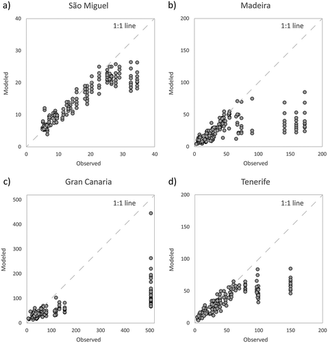
Figure 1 shows that the model over- and underpredicts the data across the four islands. Nonetheless, there is a tendency for underestimation, as shown by the predominance of sample points below the 1:1 line. In Figure 1, there are far more sample points at the lower values and a scarcity of samples at higher values. This relates directly with the normality of the distribution of data used (Table 3). In all the islands, results for the higher values show a clustered pattern due to the presence of a few outliers. Figure 1 also shows an increasing trend where there is more discrepancy in the sample points with increasing land-change values (i.e., the model performs poorly as the prediction moves from small-to-large land-change areal units). Generally, the model performs poorly in areas larger than 30 ha. A single data point, represented by the areal unit centroid, is not sufficient to model a large area, particularly when the neighboring data points from the remaining areal units have much smaller values. As a result, the model struggles to determine the land development pressure across areas dominated by outliers. It is important to note that, in the case of this study, it was essential to keep the outliers because these allow identification of very large artificial land-change areas. As such, these outliers cannot be discarded because they are paramount to the analysis of land development pressure. Among the study areas, Gran Canaria is the best example of the effect of an outlier. Gran Canaria data has an outlier with 505 ha. Figure 1(c) shows that, for the allocated points in this 505 ha artificial land-change area, the model massively under-predicts the data. Because this particular land-change area totals 505 ha, modeled values should be higher across the surface occupied by this areal unit. As the model tries to build the continuous surface, there is only one data point totaling 505 ha. However, the remaining data points have much lower values, hence the discrepancy in the surface areas dominated by outliers in every island (Figure 1).

Research indicates, “uncertainty and potential error in land-cover classification estimates may inhibit accurate assessments of land change” (Christman et al. 2015, 543). In this regard, Estoque and Murayama’s (2014) study discussed the nonstationary characteristic of land-change patterns, examining its potential effect on modeling accuracy using a geospatial approach. Therefore, users of categorical land-cover products must recognize the inherent limitations for land-change analysis (Christman et al. 2015). When analyzing Table 5, it is important to note that the choice of the interpolation method can influence the model’s goodness-of-fit measures. Moreover, centroids representing artificial land change tend to produce a clustered spatial coverage. This was, to some extent, mitigated when using the no-change sampled points that take into account the topographic resistance factor. Another issue affecting the goodness-of-fit measures is the distortion at the boundaries due to edge effects. Nonetheless, because the study areas were islands, this issue could not be addressed by having data shift from the study area.

It is important to note that IDW might not be the best algorithm to compute the surface of land development pressure. In future studies, the proposed method needs further assessment with different interpolation methods (e.g., Kriging, Spline, among others) to find the best results in terms of model fitting. Because the main goal of this article was showcasing the proposed method, there was no restrictive tolerance of estimation errors. Therefore, the modeled surfaces of land development pressure were considered acceptable in capturing the artificial land-change trend over the years.

4.3. Spatially explicit representation

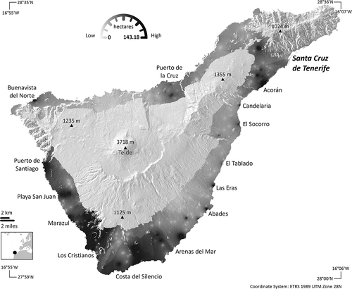
The presented method allowed for deduction of a historical trend (1990–2006) of land development pressure based on the size of observed artificial land-change areal units. This was a period marked by a rapid increase in real-estate valuations, which ended with the financial crisis of 2007–2008. Figures 2–5 represent the 30-m resolution modeled surfaces computed with the IDW interpolation with the lowest RMSE (Table 4) and constrained by a topographic resistance factor. The figures show the computed surfaces draped over a hillshade, acquired from the same DEM used as data source. Overall, the presented figures provide a spatially explicit depiction of land development pressure represented through a gradient. These results are the basis for answering the remaining research questions: What is the islands’ pattern of land development pressure? Which areas were prone to land development?

Figure 2. São Miguel’s land development pressure during the 1990–2006 period.

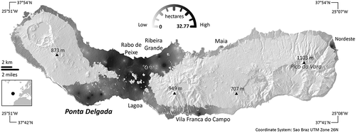
Figure 3. Madeira’s land development pressure during the 1990–2006 period.

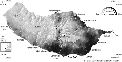
Figure 4. Gran Canaria’s land development pressure during the 1990–2006 period.

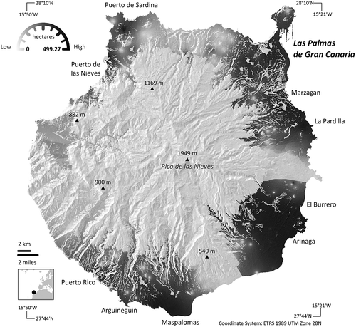
Figure 5. Tenerife’s land development pressure during the 1990–2006 period.

As expected, the lowest surface values, and thereby lowest land development pressure, occurred inland. As shown in the figures, the highest values are located along the coast, where the decay effect from the coastline is visible at a distance. One of the drawbacks of an IDW interpolation is the spatial “bull’s eye” effect, visible as lighter or darker dots. To achieve smoother surfaces, the effect could be attenuated by changing the IDW parameters. However, this would only be possible at the cost of an increased RMSE error. On the other hand, it is possible that a different interpolation algorithm (e.g., Kringing, Spline) could yield smoother interpolated surfaces whilst keeping RMSE low. Nonetheless, it was beyond the scope of this study to do a comparison of spatial interpolation methods. Therefore, to constrain RMSE values, an IDW interpolation has the drawback of producing the “bull’s eye” effect. However, this drawback also proved to be helpful because the darker “bull’s eye” acts as a hotspot of land development pressure, displayed in black in the figures. In this regard, the influence of the islands’ settlements on the surrounding landscape can be appreciated by examining the gradient’s intensity across the surfaces. Resorting to a gradient allows for an easy comparison of results, whereas “classification breaks are not comparable with other places and would be inappropriate for comparative studies” (Varanka 2010, 300).

A crucial finding in the results is that, as shown in the figures, during the 1990–2006 time frame, land development pressure had occurred not only in the vicinity of the main cities but also in smaller settlements. This indicates that there were strong LULC driving forces acting on the islands’ landscape not related to major settlements, namely tourism activity. Therefore, results indicate that there are settlements in these islands that were responsible for more land development pressure than the island’s main city, labeled in bold italic type. This process was particularly noticeable in the Spanish islands of Gran Canaria and Tenerife.

As shown in Figure 2, in São Miguel, land development pressure during 1990–2006 was higher in the northern central section of the island. Nonetheless, the island had the lowest gradient among the study areas, reaching a maximum of 32.77 ha of land development pressure during the 1990–2006 period. Because it is the least populous island among the study areas (0.14 M inhabitants), a relatively low land development pressure was expected. Moreover, an unstable climate averaging about 1000 mm (39.4 inches) of rainfall per year, and increased distance from Europe’s mainland avoided São Miguel from becoming a mass tourism destination. São Miguel’s foremost area of land development pressure had developed along the Lagoa–Rabo de Peixe/Ribeira Grande corridor (Figure 2).

In Madeira (Figure 3), land development pressure during 1990–2006 was higher in the south. The gradient shows that pressure was concentrated along the south and southeastern coast. In Madeira, between 1990 and 2006, a major area of land development pressure had developed along the Ribeira Brava–Machico corridor, encompassing the entire coastal southeastern region. Along this corridor, land development pressure had reached a maximum of 144.65 ha. Furthermore, Madeira was the best example among the case studies where its main city (Funchal, 0.11 M inhabitants) was associated to a hotspot of land development pressure. Over the years, tourism activity remained located in the city of Funchal, since there has been no resort development elsewhere in the island.

As shown in Figure 4, the southeastern region of Gran Canaria is marked by land development pressure across the area surrounding Arinaga. The intense artificial land change that has occurred in this region stands out. Consequently, the gradient of land development pressure reached 499.27 ha, the highest, by far, among the study areas. Although the Arinaga industrial area was created in the mid-1970s, the 1990s saw a significant expansion. As shown, this has been recorded in Gran Canaria’s land-change data. Another hotspot stands out in the south of the island surrounding Maspalomas, a tourist town. As such, the artificial land change occurring across this area mainly focused on tourism-related activities.

Finally, Tenerife (Figure 5) is the best example where the main city (Santa Cruz de Tenerife, 0.2 M inhabitants) was not associated with a hotspot of land development pressure. As shown in Figure 5, the south and southwestern sectors stand out as they had the main hotspots of land development pressure. Once again, empirical knowledge of the island’s landscape associates this pressure to tourism development and associated infrastructures. In Tenerife, tourism-related activities predominately converged in the south along the high-pressure areas of Figure 5. On this matter, research has confirmed the relevance of economic activity among LULC driving forces. A recent study (Cunningham et al. 2015) examined the change from undeveloped to developed land use during the real-estate bubble and subsequent bust in Massachusetts, USA. Findings from Cunningham et al. (2015) show that land development spatial patterns can be associated with economic cycles. It is important to note that the 1990–2006 period discussed in the present study was marked by rapid increases in real-estate valuations. This real-estate bubble ended with the financial crisis of 2007–2008.

To contextualize the results, it is important to note that over the last few decades, artificial land change has been the main consequence of the islands’ LULC driving forces. This increase in built-up areas has consolidated the cities. However, as the results show, it has mainly contributed to the growth of smaller settlements. To different degrees and extent, tourism-related infrastructures and improvements in road network are the main land-change driving forces in these archipelagos. Across the islands, tourism development and associated infrastructures became predominately located in the warm, clear, and dry leeward southern sides of the islands. Whereas, the visible land development pressure spreading inland is due to a continued improvement in road accessibility. This is associated with strong investment in road infrastructures in the islands, following the 1986 accession of Spain and Portugal to structural and cohesion EU funds. This led to major improvements in the islands’ road network and a decrease in travel times. This investment allowed the built-up expansion of areas further inland, some of which were inaccessible before due to the huge costs of building new road infrastructures in these rugged volcanic islands.

5. Conclusions

No standard method exists for quantifying, measuring, and evaluating land development pressure. The method outlined in this article has been successful in rescaling through an IDW interpolation, coarse land-change-derived data into a higher resolution surface of land development pressure. This surface was interpolated, assuming that land development pressure is the magnitude of a landscape’s artificial land change and that this magnitude can be represented with a gradient. The novel approach sampled ancillary data, taking into account a topographic resistance factor. IDW interpolation used this sampled ancillary information to double the data locations, confine the interpolation values, and assist the rescaling process.

Several advantages are immediately apparent from the method. (1) Data relies solely on land-use/land-cover datasets and a DEM, both available on public domain, allowing a seamless application of the method to other regions. (2) The method does not present a classification of land development pressure because the gradient of the pressure (hectares) is dependent on the observed size of artificial land-change areal units. Avoiding classification breaks and resorting to a gradient allows an easy comparison of results among distinct landscapes. (3) Rescaling the interpolated surface to a higher spatial resolution creates a visualization of the magnitude of land development pressure within the islands and its spatial variability across the landscape. On the other hand, the proposed method has some noticeable drawbacks. (1) Although encompassing large geographical extents, the method has been applied to coarse scale data and a relatively small dataset of sample points. Further testing is needed to assess the application’s performance on higher resolutions and larger datasets. (2) The method was devised using volcanic islands as study areas. Therefore, it has to be calibrated before being applied to homogenous landscapes, where topography may not play a key role.

Overall, the method allows a spatially explicit representation of observed land development pressure. The modeled surfaces should be considered as a means for further studies of land-change driving forces rather than an end in itself. Therefore, as shown, the proposed method may be a valuable asset for identifying the interactions and spatial determinants involving anthropogenic land change.

Acknowledgments

The author would like to express his sincere gratitude to Professor Javier Gutiérrez Puebla for his valuable suggestions on the early drafts of this article, and to the reviewers for their help in improving the manuscript.

Disclosure statement

No potential conflict of interest was reported by the author.

Additional information

Funding

This work was supported by the Portuguese Foundation for Science and Technology [grant number SFRH/BD/69396/2010].

References

- Abdullahi, S., B. Pradhan, S. Mansor, and A. R. M. Shariff. 2015. “GIS-Based Modeling for the Spatial Measurement and Evaluation of Mixed Land Use Development for a Compact City.” GIScience & Remote Sensing 52 (1): 18–39. doi:10.1080/15481603.2014.993854.
- Berlanga-Robles, C. A., and A. Ruiz-Luna. 2011. “Integrating Remote Sensing Techniques, Geographical Information Systems (GIS), and Stochastic Models for Monitoring Land Use and Land Cover (LULC) Changes in the Northern Coastal Region of Nayarit, Mexico.” GIScience & Remote Sensing 48 (2): 245–263. doi:10.2747/1548-1603.48.2.245.
- Bossard, M., J. Feranec, and J. Otahel. 2000. CORINE Land Cover Technical Guide: Addendum 2000. Copenhagen: European Environmental Agency.
- Boucher, A., and P. C. Kyriakidis. 2006. “Super-Resolution Land Cover Mapping with Indicator Geostatistics.” Remote Sensing of Environment 104 (3): 264–282. doi:10.1016/j.rse.2006.04.020.
- Bracken, I., and D. Martin. 1989. “The Generation of Spatial Population Distributions from Census Centroid Data.” Environment and Planning A 21 (4): 537–543. doi:10.1068/a210537.
- Britz, W., P. H. Verburg, and A. Leip. 2011. “Modelling of Land Cover and Agricultural Change in Europe: Combining the CLUE and CAPRI-Spat Approaches.” Agriculture, Ecosystems & Environment 142 (1–2): 40–50. doi:10.1016/j.agee.2010.03.008.
- Burrough, P. A. 2001. “GIS and Geostatistics: Essential Partners for Spatial Analysis.” Environmental and Ecological Statistics 8 (4): 361–377. doi:10.1023/A:1012734519752.
- Burrough, P. A., and R. A. McDonnell. 1998. “Creating Continuous Surfaces from Point Data.” In Principles of Geographic Information Systems, edited by P. A. Burrough, M. F. Goodchild, R. A. McDonnell, P. Switzer, and M. Worboys, 98–131. Oxford: Oxford University Press.
- Christman, Z., J. Rogan, J. R. Eastman, and B. L. Turner II. 2015. “Quantifying Uncertainty and Confusion in Land Change Analyses: A Case Study from Central Mexico Using MODIS Data.” GIScience & Remote Sensing 52 (5): 543–570. doi:10.1080/15481603.2015.1067859.
- Cunningham, S., J. Rogan, D. Martin, V. DeLauer, S. McCauley, and A. Shatz. 2015. “Mapping Land Development through Periods of Economic Bubble and Bust in Massachusetts Using Landsat Time Series Data.” GIScience & Remote Sensing 52 (4): 397–415. doi:10.1080/15481603.2015.1045277.
- Epstein, J. M. 2008. “Why Model?.” Journal of Artificial Societies and Social Simulation 11 (4): 12.
- Estoque, R. C., and Y. Murayama. 2014. “A Geospatial Approach for Detecting and Characterizing Non-Stationarity of Land-Change Patterns and Its Potential Effect on Modeling Accuracy.” GIScience & Remote Sensing 51 (3): 239–252. doi:10.1080/15481603.2014.908582.
- Fernández-Palacios, J. M., L. De Nascimento, R. Otto, J. D. Delgado, E. García-del-Rey, J. R. Arévalo, and R. J. Whittaker. 2011. “A Reconstruction of Palaeo-Macaronesia, with Particular Reference to the Long-Term Biogeography of the Atlantic Island Laurel Forests.” Journal of Biogeography 38 (2): 226–246. doi:10.1111/jbi.2011.38.issue-2.
- Foley, J. A., R. DeFries, G. P. Asner, C. Barford, G. Bonan, S. R. Carpenter, F. S. Chapin, et al. 2005. “Global Consequences of Land Use.” Science 309 (5734): 570–574. doi:10.1126/science.1111772.
- Gardner, R. H., T. R. Lookingbill, P. A. Townsend, and J. Ferrari. 2008. “A New Approach for Rescaling Land Cover Data.” Landscape Ecology 23 (5): 513–526. doi:10.1007/s10980-008-9213-z.
- Jaimes, N. B. P., J. B. Sendra, M. G. Delgado, and R. F. Plata. 2010. “Exploring the Driving Forces behind Deforestation in the State of Mexico (Mexico) Using Geographically Weighted Regression.” Applied Geography 30 (4): 576–591. doi:10.1016/j.apgeog.2010.05.004.
- Jarnagin, S. T. 2004. “Regional and Global Patterns of Population, Land Use, and Land Cover Change: An Overview of Stressors and Impacts.” GIScience & Remote Sensing 41 (3): 207–227. doi:10.2747/1548-1603.41.3.207.
- Long, H., G. Tang, X. Li, and G. K. Heilig. 2007. “Socio-Economic Driving Forces of Land-Use Change in Kunshan, the Yangtze River Delta Economic Area of China.” Journal of Environmental Management 83 (3): 351–364. doi:10.1016/j.jenvman.2006.04.003.
- Nagendra, H., D. K. Munroe, and J. Southworth. 2004. “From Pattern to Process: Landscape Fragmentation and the Analysis of Land Use/Land Cover Change.” Agriculture, Ecosystems & Environment 101 (2–3): 111–115. doi:10.1016/j.agee.2003.09.003.
- Peneva-Reed, E. 2014. “Understanding Land-Cover Change Dynamics of a Mangrove Ecosystem at the Village Level in Krabi Province, Thailand, Using Landsat Data.” GIScience & Remote Sensing 51 (4): 403–426. doi:10.1080/15481603.2014.936669.
- Pijanowski, B. C., D. G. Brown, B. A. Shellito, and G. A. Manik. 2002. “Using Neural Networks and GIS to Forecast Land Use Changes: A Land Transformation Model.” Computers, Environment and Urban Systems 26 (6): 553–575. doi:10.1016/S0198-9715(01)00015-1.
- Temme, A. J. A. M., and P. H. Verburg. 2011. “Mapping and Modelling of Changes in Agricultural Intensity in Europe.” Agriculture, Ecosystems & Environment 140 (1–2): 46–56. doi:10.1016/j.agee.2010.11.010.
- Van Vuuren, D. P., S. J. Smith, and K. Riahi. 2010. “Downscaling Socioeconomic and Emissions Scenarios for Global Environmental Change Research: A Review.” Wiley Interdisciplinary Reviews: Climate Change 1 (3): 393–404.
- Varanka, D. 2010. “Interpolating a Consumption Variable for Scaling and Generalizing Potential Population Pressure on Urbanizing Natural Areas.” In Geospatial Analysis and Modelling of Urban Structure and Dynamics, edited by B. Jiang and X. Yao, 293–310. Netherlands: Springer.
- Verburg, P. H., C. J. E. Schulp, N. Witte, and A. Veldkamp. 2006. “Downscaling of Land Use Change Scenarios to Assess the Dynamics of European Landscapes.” Agriculture, Ecosystems & Environment 114 (1): 39–56. doi:10.1016/j.agee.2005.11.024.
- West, T. O., Y. L. Page, M. Huang, J. Wolf, and A. M. Thomson. 2014. “Downscaling Global Land Cover Projections from an Integrated Assessment Model for Use in Regional Analyses: Results and Evaluation for the US from 2005 to 2095.” Environmental Research Letters 9 (6): 064004. doi:10.1088/1748-9326/9/6/064004.
- Wickham, J. D., R. V. O’Neill, and K. B. Jones. 2000. “Forest Fragmentation as an Economic Indicator.” Landscape Ecology 15 (2): 171–179. doi:10.1023/A:1008133426199.
- Wu, C., and A. T. Murray. 2005. “A Cokriging Method for Estimating Population Density in Urban Areas.” Computers, Environment and Urban Systems 29 (5): 558–579. doi:10.1016/j.compenvurbsys.2005.01.006.