Channel bar feature extraction for a mining-contaminated river using high-spatial multispectral remote-sensing imagery

Abstract

Mapping and monitoring changes of geomorphological features over time are important for understanding fluvial process and effects of its controlling factors. Using high spatial resolution multispectral images has become common practice in the mapping as these images become widely available. Traditional pixel-based classification relies on statistical characteristics of single pixels and performs poorly in detailed mapping using high resolution multispectral images. In this work, we developed a hybrid method that detects and maps channel bars, one of the most important geomorphological features, from high resolution multispectral aerial imagery. This study focuses on the Big River which drains the Ozarks Plateaus region in southeast Missouri and the Old Lead Belt Mining District which was one of the largest producers of lead worldwide in the early and middle 1900s. Mapping and monitoring channel bars in the Big River is essential for evaluating the fate of contaminated mining sediment released to the Big River. The dataset in this study is 1 m spatial resolution and is composed of four bands: Red (Band 3), Green (Band 2), Blue (Band 1) and Near-Infrared (Band 4). The proposed hybrid method takes into account both spectral and spatial characteristics of single pixels, those of their surrounding contextual pixels and spatial relationships of objects. We evaluated its performance by comparing it with two traditional pixel-based classifications including Maximum Likelihood (MLC) and Support Vector Machine (SVM). The findings indicate that derived characteristics from segmentation and human knowledge can highly improve the accuracy of extraction and our proposed method was successful in extracting channel bars from high spatial resolution images.

Keywords:

• feature extraction
• object-based
• classification
• images
• river

Introduction

Channel bars are common landforms used for geomorphic and sediment assessments for rivers worldwide (Edwards et al. 1999; Gurnell et al. 2001; Gilvear and Willby 2006). They are formed by fluvial deposition of sediments within the river channel and related to sedimentary dynamics such as through mining, dredging and transport regimes (Schumm 2005). Any modification of their occurrence and state will have implications for the characteristics and variations of sediment flux (Tubino and Seminara 1990; Seminara, Tubino, and Zardi 2001; Abad and Garcia 2009; Hooke and Yorke 2011). Mapping and monitoring the natural locations, numbers and dynamics of channel bars are essential in understanding and carrying out studies on fluvial processes and effects of human and geomorphic controlling factors (Wallick et al. 2011). For example, planform analyses of channel bars can be used to classify geomorphic forms (Rosgen 1996, 2006; Schumm 2005), monitor channel disturbances (Jacobson and Gran 1999; Martin and Pavlowsky 2011) and evaluate causes of geomorphic instability in river systems (Montgomery and MacDonald 2002). Typically, field surveys such as GPS positioning (Brasington, Rumsby, and McVey 2000) are employed to map channel bar data such as its size and location. However, due to land access or vegetation constraints, it is generally limited in terms of spatial scope and time flexibility. The new generation of high spatial resolution multispectral data (e.g., SPOT 5, GeoEye-1 and WorldView-2) offers an alternative, yet cost-efficient way of monitoring bar features, given its ability to cover much more details in broader spatial extents and in quick succession at reasonable costs. This in turn enables researchers to study channel network features, increase the accuracy of environmental transport models (e.g., water, sediment and nutrients) and inform decisions for targeting conservation practices by using data in conjunction with modeling (Wilcock 2001; Nyarko et al., 2015).

While finer resolution or larger scale sensors provide more details about specific features of interest, feature extraction using classification techniques becomes more complex (Myint 2006; Güneralp, Filippi, and Hales 2013; Lu et al., 2014). As spatial resolution increases, more and more small objects become visible with higher level of details. This in turn leads to variability increase in internal spectral responses of objects and consequently reduces the spectral discrepancies between object classes. Additionally, spectral resolution is often limited with this type of images, typically having only a few bands. For example, GeoEye-1 and QuickBird images can provide a very high spatial resolution of less than half meter, but only a coarse spectral resolution of four bands (blue, green, red and near infrared). Therefore, different materials might exhibit similar spectral signatures on high spatial resolution images, making it difficult to discriminate objects using spectral information alone (Kumar and Castro 2001; Herold, Gardner, and Roberts 2003; Kumar and Sinha 2014). Due to the aforementioned characteristics, traditional pixel-based classifiers such as maximum likelihood classification (MLC) and support vector machine (SVM) do not perform well on high spatial resolution images (Hay, Niemann, and McLean 1996; Walter 2004; Lillesand, Kiefer, and Chipman 2008; Weng 2009; Zhang and Xie 2013; Ziaei, Pradhan, and Mansor 2014). The widely used MLC employs statistical probability to label a pixel to a class based on the pixel’s spectral similarity. With the increasing intra-class spectral variability on high spatial resolution images, individual pixels are classified differently from their neighbors. The classification results often show a salt-and-pepper effect with reduced classification accuracy (Friedl and Brodley 1997; Jensen 2005; Otukei and Blaschke 2010). SVM is a supervised, non-parametric statistical-learning technique. It advances statistical algorithm to minimize misclassification by employing so-called optimal separation hyperlanes – the decision boundary obtained in the training steps. However, the classification results are sensitive to the choice of kernels and the settings of other parameters (Zhu and Blumberg 2002; Mountrakis, Im, and Ogole 2011; Güneralp, Filippi, and Hales, 2013; Mui, He, and Weng 2015; Lin and Yan 2016).

To tackle this H-resolution problem referred in the work of Yu et al. (2006), researchers then attempted to develop approaches that can take the advantages of the high spatial resolution of sensors and use additional information to supplement spectral information for image analysis. Object-based image analysis (OBIA) techniques are particularly appealing in the remote-sensing field due to their ability to incorporate ancillary information into the classification process (Hay, Niemann, and McLean 1996; Fisher 1997; Blaschke and Strobl 2001; Blaschke, Burnett, and Pekkarinen 2004; Qiu, Wu, and Miao 2014). Typically OBIA starts with a segmentation process to group pixels into objects based on certain homogeneity criteria. Numerous segmentation algorithms have been developed in literature. For instance, region-based segmentation methods provide closed boundary of objects and make use of relatively large neighborhoods for decision making (Beaulieu and Goldberg 1989; Adams and Bischof 1994; Feitosa et al. 2011). Hybrid segmentation methods combine edge or gradient information with region growing (Gambotto 1993; Lemoigne and Tilton 1995). The ECHO algorithm uses statistical testing followed by a maximum likelihood object classification for image segmentation (Landgrebe 1980). To further improve the performance, many studies then introduced ancillary information into the analysis. Examples of such information include image texture (e.g. fine, medium, coarse), contextual information (e.g. connectivity, adjacency, proximity) and geometric attributes (e.g. size, shape, border length, directionality) of features (Baatz and Schäpe 2000; Navulur 2007; Im, Jensen, and Tullis 2008; Blaschke 2010). For instance, Shackelford and Davis (2003) incorporated texture measures and a length–width contextual measure to improve the discrimination between spectrally similar “Road” and “Building” urban land-cover types. Ivits et al. (2005) derived indices from segmented homogeneous patches ranging from old-growth forests to intensive agricultural landscapes. The derived patch indices were later used to classify 96 sample plots in Switzerland. Platt and Rapoza (2008) investigated the typical four components in object-based analysis, namely the segmentation procedure, the nearest neighbor classifier, the integration of expert knowledge and feature space optimization. They found that the combination of the first three components offered substantially improved classification accuracy over a pixel-based method. Many studies have evaluated OBIA techniques and found that they can generate better accuracy compared with traditional pixel-based method (e.g., Kamal and Phinn 2011; Zhang and Xie 2013). A recent review of OBIA is given by Blaschke et al. (2014). They formalized core concepts of OBIA and concluded that OBIA is desirable in processing high spatial resolution image data.

While interpreting high-spatial resolution imagery, experienced photointerpreters often outperform computer algorithm-based approaches, although the process can be time-consuming and subjective. This is due to our ability to make inferences based not only on spectral properties (Moreira, Teixeira, and Galvão 2015; Xun and Wang 2015), but also on knowledge about object information such as shape, texture, patterns, shadows and spatial relationships (Laliberte et al. 2004; Paine and Kiser 2012). Knowledge-based classification methods have been developed to incorporate human knowledge into classifier and improve classification accuracy. Expert knowledge can be expressed in several ways for the use of knowledge-based classifiers. For example, the commonly used approach is rule-based (also referred to as production rules). Myint (2006) developed different expert rules to delineate buildings, impervious surface, swimming pools, lakes and ponds from a QuickBird image. Kass, Notarnicola, and Zebisch (2011) developed rules based on different texture-based measurements of about half of the image objects and then used these rules to classify the remaining objects.

Regarding channel bars, researchers have found their spectral properties can potentially be confused with some seemingly different features such as river banks, stabilized tailings piles or bare soils (Gilvear, Davids, and Tyler 2004). The constituent profiles and optical properties of channel bars can also be influenced by the formation and succession of vegetation on bars (Dugdale, Carbonneau, and Cambell 2010; Hooke and Yorke 2011). Additionally, remote-sensing extraction of channel bars involves similar difficulties that may be encountered with man-made features such as roads, buildings and parking lots. This includes the existence of obstructions (e.g., bushes) and shadows which in remote-sensor images can pose problems that are difficult to address and can lead to inaccurate mapping results (Güneralp, Filippi, and Hales 2013). Additionally, misclassification error can occur as a function of the variability in spectral optical properties of depositional features (e.g., gravels, sands or mine sediments) that constitute channel bars. Hence, accurately classifying this type of geomorphological features from high-resolution image data remains a challenge despite significant advances in remote-sensing technologies. For example, Gilvear, Davids, and Tyler (2004) applied pixel-based classification to classify color aerial photography and multi-spectral images for the River Tummel, Scotland. They compare the classification accuracy with field survey. The results demonstrated a significant confusion between gravel bars (termed channel bars in our approach for the sake of generality), bare soil and riprap where 37% of the gravel bars were misclassified as riprap. In recent years, we have witnessed considerable progress using Airborne LiDAR in river valleys for topography and hydro-morphology. Pénard and Morel (2012), for example, derived 0.25 m resolution DTM from an airborne LiDAR survey and developed a method for automatic segmentation of a river channel into distinct hydro-morphological entities such as water, gravel bars and banks. Hilldale and Raff (2008) show the effectiveness of bathymetric LiDAR for immersed topography. However, the large datasets of 3D point clouds require challenging post-processing (Pan et al. 2015).

In this work, we propose a hybrid method that combines object-based and knowledge-based classification to extract geomorphological features at the local scale using high spatial resolution images. Particularly, we are interested in channel bars as they are essential in understanding and carrying out studies on fluvial processes and effects of human and geomorphic controlling factors (Wallick et al. 2011). Specifically, we evaluate the effectiveness of image segmentation and human knowledge in improving channel bar boundary extraction. By incorporating spectral characteristics of single pixels, those of their surrounding contextual pixels and spatial relationships of objects, this method offers better performance in extracting channel bars from high spatial resolution multispectral remotely sensed images. Additionally, we quantitatively evaluated the proposed method by comparing the extracted boundaries against the reference data. Traditional pixel-based classifications including MLC and SVM were also tested on the same dataset and compared with our proposed method. The results show that the hybrid method was successful in extracting channel bars from high spatial resolution images and characteristics derived from segmentation and human knowledge can highly improve the accuracy of extraction.

Study area and data

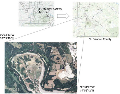
The study site is located in St. Francois County, Missouri (Figure 1). It covers an area of about 5.6 km² including a segment of the Big River between the towns of Leadwood and Desloge (upper left longitude 90°33′41″ W and latitude 37°53′49″ N, lower right longitude 90°31′47″ W and latitude 37°52′42″ N). The Big River drains about 675 km² of the Ozark Highlands’ ecoregion and covers the largest historical lead-mining area in the United States (USGS, 1998). Past and ongoing releases of mill effluents, mineral wastes and mining sediments have resulted in the contamination of channel sediment and floodplain deposits in the Big River (Pavlowsky, Owen, and Martin 2010). Channel bars in the Ozarks region are typically composed of sand and gravel with cobbles in some places (Panfil and Jacobson 2001). Bar sediment was introduced to the river from natural erosion, early settlement land disturbances and mining operations (Jacobson and Primm 1994; Pavlowsky, Owen, and Martin 2010). Channel bar deposition and related planform effects on stream ecology and geomorphic behavior are of great interest to managers and scientists in the Ozarks region (Jacobson and Gran 1999; Martin and Pavlowsky 2011; Owen, Pavlowsky, and Womble 2011). Moreover, bar sediments in the Big River contain more than 1000 ppm lead which threatens aquatic life, and therefore the locations of contaminated sediment needs to be monitored (Pavlowsky, Owen, and Martin 2010). Here, we used aerial images acquired through National Agriculture Imagery Program (NAIP) in this work. NAIP imagery is a popular and useful data source due to its nationwide coverage, low cost to the public, frequent update and high spatial resolution (Maxwell et al. 2014). Our study site is covered by NAIP imagery acquired on 1 July 2010. The dataset is a Digital Orthophoto Quarter Quads (DOQQs) product rectified in the Universal Transverse Mercator (UTM) coordinate system, NAD83. The image has 1 m spatial resolution and is composed of four bands: Red (Band 3), Green (Band 2), Blue (Band 1) and Near-Infrared (Band 4). Even though the study area is relatively a small portion of the county, its image data is sizeable (2832 rows by 1985 columns) due to its fine spatial resolution covering approximate 5.6 square kilometers.

Figure 1. Study site, located in St. Francois County, Missouri.

Methods

In this study, we focus on the separation of channel bars from other land-cover types present in the image. The proposed hybrid method is illustrated in Figure 2. We started by segmenting image pixels into homogenous and unified regions/objects. It was followed by a three-step knowledge-based classification. First, spectral filtering was applied to classify the segmented image to water bodies and non-water bodies. Second, non-water body areas are further broken down based on revised NDVI. Third, spatial topology between interested objects were tested, followed by spatial merging and filtering to eliminate extreme small or large objects. Algorithms in the object base are developed under eCognition Developer, commercial software offered by Trimble^®. We leverage its powerful tools and extend its core functions with expert knowledge in our proposed approach. To demonstrate if spectral information alone is effective to fulfill the task, we used the spectra of seventy five randomly selected points from identified classes to examine if they can be accurately discriminated. Following the analysis, our proposed method is presented in details. We then classified the image using traditional pixel-based classification including MLC and SVM. The accuracies of these two traditional pixel-based classification methods were compared with ours to thoroughly evaluate the effectiveness of our proposed hybrid approach.

Figure 2. Flowchart of the developed hybrid approach.

Spectral separation analysis for land-cover classes

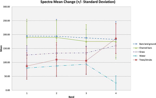
The selected land-cover classes that we identified for the study include bare land ground (i.e., impervious surfaces like roads, buildings and other land surfaces without vegetation covered), trees/shrubs, channel bars, grass and water. We randomly selected fifteen points for each identified land-cover type to be used. To evaluate the spectral separation between categories, we employed the coincident spectral plot approach which is popular in traditional pixel-based classification for training set refinement (Figure 3). The diagram facilitates the comparison of spectral distribution between different class types. It illustrates the mean spectral response of each class and the variance of the distribution (± standard deviations shown by colored bars) in each spectral band (Lillesand, Kiefer, and Chipman 2008). It is obvious that many classes in our study area have similar spectral responses throughout all four bands, for example, the bare land ground with channel bars and the tree/shrubs with grass. Particularly, the spectra mean values of the bare land ground class are close to those of the channel bars, especially in Band 1 and Band 2. In addition, their spectral distributions overlap greatly within the standard deviations, indicating strong spectral similarity between these two classes. Figure 3 also shows overlapping in spectral distributions between the channel bars and the other two classes – the grass and the trees/shrubs. Apparently this type of spectral confusion is introduced by vegetation growing on the surface of channel bars.

Figure 3. Coincident spectral plots for randomly selected points obtained for different cover types.

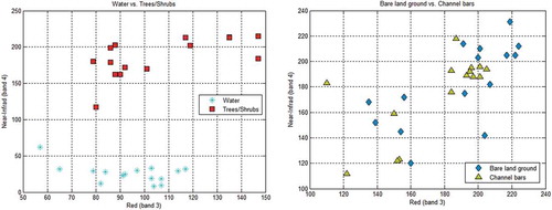
The diagram also shows which combination of bands might be best for separating classes because of relative reversals of spectral response (such as Band 3 and Band 4 for water and trees/shrubs separation). Two-dimensional scatter diagrams are used for this purpose to better analyze the spectral response patterns of classes. The scatter diagram plots spectral responses in one band vs. these in another. These two spectral responses locate each pixel value in the two dimensional “measurement space” of the graph. For example, in Figure 4, the Band 3 spectral responses have been plotted on the x-axis and the Band 4 spectral responses on the y-axis. Figure 4a shows that the water class has lower variance in spectral properties than the trees/shrubs. In addition, these two classes have no overlapping in the graph, indicating that they are not correlated in Band 3 and Band 4. In comparison, spectral responses of pixels in both bare land ground and channel bars vary greatly and overlap significantly as illustrated in Figure 4b. This pattern indicates that these two classes are not able to be well separated using Band 3 and Band 4. With such exploratory analysis for all five classes in various combination of bands using the randomly selected seventy five points, the scatter diagrams indicate that using the spectra information alone, as in the classical approaches, may not be effective for separating channel bars, especially from the class of bare land ground.

Figure 4. Scatter plots (Band 3 vs. Band 4) for randomly selected points obtained for two pairs of cover types: (a) left: water vs. trees/shrubs; (b) right: bare land ground vs. channel bars.

Channel bar extraction

Channel bar sediment accumulations extend above bed elevation which are composed of sand or gravel deposited by flow within or along the sides of the river channel. Active channel bar surfaces are typically exposed at low water with no/sparse vegetation cover (Hooke and Yorke 2011). Thus, their spatial and textural characteristics can be summarized as: (1) channel bars have the same spectra distribution in all bands as the bare land ground (Figure 2); (2) they are located within or adjacent to the water; (3) vegetation cover varies but usually lacks or is sparse. In this article, we incorporate these spatial and textural characteristics into object-based analysis to develop a hybrid approach through a set of rules. The developed algorithms can automatically extract channel bars from high spatial resolution multispectral images and it composes of three key modules: image segmentation, classification of water bodies and grounds with no/sparse vegetation and extraction of channel bars, which are illustrated in details in following subsections.

Image segmentation

We initiate the method by segmenting the whole aerial image into homogenous and unified regions/objects. Image pixels with similar spectral and spatial properties are grouped into an object. We use a segmentation algorithm available in eCognition known as the multi-resolution segmentation (Baatz and Schäpe 2000). It is conducted by the Fractal Net Evolution Approach (FNEA) which is a bottom-up region growing technique. FNEA starts with one-pixel image objects and pairwise merges into larger ones. The process stops when average spectral and spatial heterogeneity of image objects weighted by their size in pixels are minimized (Baatz and Schäpe 2000; Benz et al. 2004). We adopt this method because of its fast execution and ability to take account of both spatial and spectral information in high-resolution remotely sensed imagery.

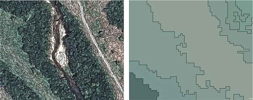
In the multi-resolution segmentation process, three key parameters are used to control the object generation from pixels, namely, shape, compactness and scale. The shape factor adjusts the shape of objects vs. the spectral homogeneity. A lower shape factor value gives less weight on shape and more attention on spectrally more homogeneous pixels. The result will be jagged object polygons with narrow spectral range. A higher value, in contrast, emphasizes on shape information, leading to amorphously shaped polygons that do not adhere to the color homogeneity. The compactness factor determines the object shape between smooth boundaries and compact edges. It is used only when the shape factor is larger than zero. The scale parameter is the most critical parameter of image segmentation. It controls the relative size of output feature polygons that matches the user’s required level of detail. Figure 5 illustrates the segmentation results of a subset image at two scale levels implemented in eCognition. Using larger scale size outputs larger homogeneous objects (Figure 5b), whereas a smaller scale will result in smaller objects (Figure 5a). The decision on the level of scale depends on the size of object required to achieve the goal. In this study, we tested different scale values and evaluated qualitatively. According to our observation, the scale parameter 20 is more suitable along with other default parameters to extract channel bars for this study, resulting in 33,277 objects for the whole image.

Figure 5. Segmentation comparison on the same subset of image: (a) left: scale parameter 10; (b) right: scale parameter 50.

Classification of water bodies

We employed our expert knowledge to define rules and constraints in the membership function classifier to identify water bodies (including the big river and ponds) in the study area. The membership function describes the intervals of feature characteristics which determine whether the objects belong to a particular class or not. For water bodies, the most noticeable characteristics is that almost all of the incident near-infrared radiant is absorbed with negligible scattering taking place, producing low reflectance values of their pixels in near-infrared band. In our study area, the reflectance values of pixels (a.k.a. pixel values) of water bodies range approximately from 10 to 60 in the near-infrared band (Band 4), which is extremely low in comparison to pixel values of other four classes in this band. Note that in Bands 1–3, the reflectance interval of water body pixels is approximately 45– 117. This range is different from classes of bare land ground and channel bars, while it significantly overlaps those of trees/shrubs and grass. It is straightforward, therefore, to extract the water bodies using the near-infrared band. We found that the mean of pixel values in the near-infrared band that are less than 60 can effectively identify water bodies. It is used as our expert knowledge rule to capture water bodies.

Classification of bare ground

This component was to identify bare ground effectively. Bare ground here refers to any ground with sparse or no vegetation covered. Note that this includes the bare land ground such as roads, building rooftops, bare soil, unmanaged soil as well as the channel bars since they are all lack of vegetation. After identifying bare ground, we then separate channel bars from it. As we discussed previously, the image used for this study area is provided by NAIP. Such image is acquired during the agricultural growing season. Healthy vegetation absorbs most of the visible light that hits it, and reflects a large portion of the near-infrared light. Unhealthy or sparse vegetation reflects more visible light and less near-infrared light. The Normalized Difference Vegetation Index (NDVI) is calculated to quantify the density of plant growth on the ground. It is expressed as

(1)

where NIR is the reflectance measured in the near-infrared band and red is the reflectance in the red band (Ustin 2004). Such reflectance is measured from individual pixels. In our hybrid approach, image segmentation has been performed before classification taking place. Pixels in the image have been grouped into homogeneous objects based on certain criteria so that more meaningful characteristics can be extracted from the resulting objects. Therefore, Equation (1) is not suitable for our approach. We revise it to use mean reflectance values of image objects in NIR and Red bands as below:

(2)

Note that the NDVI derived from Equation (2) quantifies the plant density for each image object instead of that for individual pixels as in Equation (1). This is important in improving the classification accuracy because of (1) significantly reduced “salt-and-pepper” effects due to noise and details provided by the high-resolution imagery; and (2) more meaningful characteristics for classes (Blaschke 2010). It is found that the NDVI values less than 0.04 indicate bare ground with no/sparse vegetation. We use it as the expert knowledge rule to classify bare ground, i.e., NDVI ≤0.04.

Extraction

After the aforementioned process, objects in the segmented images are classified as water bodies, bare ground or unlabeled. Due to lack of vegetation, objects which should be channel bars are classified as bare ground from NDVI rule set. Previous spectral analysis indicates that there is significant spectral signature confusion between channel bars and other bare ground such as bare soil. However, if an object is adjacent or within a short distance to water bodies, then the object is more likely to be a channel bar than other bare ground. We model this spatial topology (proximity) as distance in the membership function. For each unlabeled object in the segmented image, its distance to identified water bodies is calculated as the number of pixels. Objects within a short distance are classified as channel bars. As the water bodies include the big river and ponds/lakes in the study area, some bare ground is close to ponds/lakes, but having extremely large (e.g., stabilized piles) or small (e.g., noises) area in object geometry than channel bars. Consequently, we merge the identified channel bar objects from distance rule and employ area size as a feature to remove those with extreme values. The following describes the expert knowledge rules that are used to refine bare ground to extract channel bars:

1. Distance to the water bodies ≤80 m (and)

2. Area size between 120 m² and 20000 m².

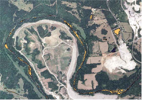
The output map of the object-based approach is shown in Figure 6.

Figure 6. Channel bar extraction by object-based approach (represented by polygons).

Classic pixel-based classification

For comparison purposes, we performed two classifiers widely used in remote sensing (San Miguel-Ayanz and Biging 1996; Mountrakis, Im, and Ogole 2011) on the same image data: MLC and SVM. Even though only the channel bar is the feature of interest to compare, to better illustrate the limitations of pixel-based classifiers we use the same land-use and land-cover categories as those identified in the spectral analysis, including channel bars.

In MLC, we selected 3 to 5 training samples per each category that represent the spectral characteristics of features in that category based on the visual interpretation of the image. The spectral responses from the training samples are then combined into a single spectral signature for each category. With such trained spectral signatures, MLC then classifies each pixel into the most probable land-cover class using a parametric classification. We performed its accuracy assessment by sampling a subset of pixels that are assumed to be representative (Jensen 2005; Lillesand, Kiefer, and Chipman 2008). The ground reference information is from visually interpreting the high spatial resolution imagery used for this study. Typically, a minimum of 50 sample points (pixels) for each land-cover category are suggested to produce the error matrices (Congalton and Green 1999). We used a stratified random sampling approach to generate 300 sample points that led to approximately 60 points per class (5 classes). The variations of sample size are due to the proportion of the corresponding type in the image. From the error matrix, we can generate overall accuracy, producer’s accuracy and user’s accuracy for each category, and kappa coefficient.

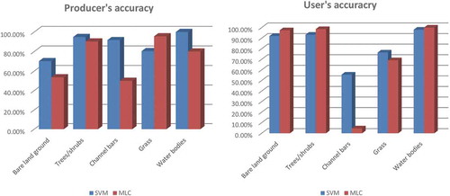
SVM is performed on the same data using Radial Basis Function (RBF). It should be noted that SVM classifier with RBF kernel typically has parameters that need to be estimated with various methods in order to identify different objects in high-spatial multispectral images (Lin and Yan 2016; Gao et al. 2015; Xun and Wang 2015). In this work, we adopted the parameters suggested by ENVI 4.5 in its default setting with gamma as 0.25 and penalty 100 (Wu, Lin and Weng, 2004; Chang and Lin 2001, 2011) for the classification. We randomly selected a number of pixels, and then picked 74 pixels among them by visual inspection that are proportional to the area of each class. Together we selected 15 pixels for bare land ground, 31 pixels for tree shrubs, 9 pixels for the sediment bars, 14 pixels for grass and 5 pixels for water body. We further programmed to draw 80% from these pixels by each class as training samples and proceeded with SVM classification, and then used the rest 20% pixels to assess the accuracy. By repeating this process ten times, the error matrices are averaged to produce the averaged producer’s and user’s accuracy (Figure 7) for SVM classification.

Figure 7. Classification accuracy from MLC and SVM.

Results and discussion

Pixel-based classification accuracy

Table 1 shows the generated error matrices and classification accuracies from MLC. It can be observed that the MLC classifier produced high overall accuracy (82.33%) and kappa coefficient (0.73) for the identified five classes. However, the user’s accuracy produced by the channel bars category is extremely low, only 4.55%. Many different sample points mistakenly classified as sediment bars actually belong to other classes, a majority of which should be bare land ground. This is expected because there was significant signature confusion among bare land ground and channel bars as discussed earlier. The bare land ground and channel bars also produced very low producer’s accuracies (53.52% and 50.00%, respectively). Many sample points that should belong to bare land ground are mistakenly allocated to channel bars or grass. It should be pointed out that other classes including trees/shrubs, grass and water bodies produced relatively high producer’s and user’s accuracies since their spectral responses are differentiable. Grass has relatively lower user’s accuracy (69.15%) because ground with sparse grass present similar spectral signatures as grass. Many sample points that were classified as grass are actually bare land ground having sparse vegetation covered. Figure 7 listed classification accuracy of SVM along with MLC. It shows SVM achieved a better accuracy with 84% accuracy overall and 55.56% user’s accuracy for classifying the channel bars. SVM advances the traditional statistical algorithms by employing optimal separating hyperplanes to better separate pixels into land-cover classes. Supplemented with various kernel functions and provided with proper training samples, SVM is able to optimize the statistical boundaries among tree shrubs, grass and water body from others, given their distinctive spectral features. However, the user’s accuracy for the channel bars fall short inevitably because its spectral characteristics sometimes are almost inseparable from the bare land ground, resulting features which are not channel bars are classified into this class.

Table 1. Confusion matrix and accuracy assessment from MLC classifier.

Classified data	Reference data						Producer’s accuracy (%)	User’s accuracy (%)
	Bare land ground	Trees/shrubs	Grass	Channel bars	Water bodies	Total
Bare land ground	38	0	1	0	0	39	53.52%	97.44%
Trees/shrubs	0	139	1	0	1	141	90.26%	98.58%
Grass	13	15	65	1	0	94	95.59%	69.15%
Channel bars	20	0	1	1	0	22	50.00%	4.55%
Water bodies	0	0	0	0	4	4	80.00%	100%
Total	71	154	68	2	5	300
Overall classification accuracy = 82.33%
Overall Kappa Statistics = 0.73

Hybrid classification accuracy

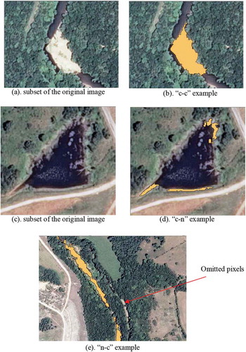
To perform the classification accuracy assessment, three indices introduced by Zhao et al. (2011) are utilized. The first index is termed “c-c” representing pixels which are correctly classified as “channel bars”. Another index is called “c-n” indicating pixels which were improperly included in the “channel bars” category. The third index is referred as “n-c” which denotes pixels that should have been classified as “channel bars” but have been missed. To determine the first two indices, the extracted channel bars were exported in the vector format (polygons) with area attribute (in pixels). The polygons were then overlaid on the original image and visually interpreted against the image as ground truth. The third index “n-c” index can be obtained by manually checking objects along the river which were omitted from “channel bars”. Figure 8 demonstrates examples (orange = extracted channel bars) for these three cases from our extraction result.

Figure 8. Examples in “c-c”, “c-n” and “n-c” derived by the object-based approach.

It should be noted that in this work our proposed approach focuses on the extraction of channel bars. Therefore, in evaluating the performance of the proposed approach, we only compare the accuracies of the “channel bars” category achieved from our approach and the two pixel-based approaches. Prior discussion shows pixel-based classifier produced exceptionally low accuracy for channel bars, particularly using MLC (50% in producer’s accuracy and 4.55% in user’s accuracy). SVM can generate higher accuracy in producer’s (91.67%), but still remains low in user’s accuracy (55.56%). For our hybrid approach, we examine every pixel in the classified category of channel bars against their ground reference information obtained by interpreting the high-resolution aerial image data using fundamental elements of image interpretation (Jensen 2005). As a result, the producer’s accuracy of channel bars extracted for our approach can be calculated by dividing the area (in pixels) of correctly classified objects (s-s) by the total area (in pixels) of channel bars in the study area. Likewise, the corresponding user’s accuracy can be calculated by dividing the total area of correctly classified objects by the total area of objects that are classified in that category. This type of assessment reflects the actual accuracy of an extraction output whether the investigated category’s pixel is accurately identified. From Table 2, it can be observed that object-based classifier produced much higher accuracy (94.04% in producer’s accuracy, 74.17% in user’s accuracy). This indicated object-based classifier is more robust in terms of separating categories having spectral signature confusion.

Table 2. Classification accuracy from proposed hybrid method – “channel bars” category.

	c-c	c-n	n-c
Pixels	55404	19299	3513
Producer’s accuracy: 55404/(55404 + 3513) = 94.04%
User’s accuracy: 55404/(55404 + 19299) = 74.17%

Figure 8d shows that pixels close to water bodies such as lakes or even puddles on the land are incorrectly classified into bars. This produced relatively low user’s accuracy (74.17%) comparing to the producer’s accuracy (94.04%). However, these water bodies are usually on land areas outside the flood plain of the Big River. Ancillary layers such as the 100-year flood plain from the FEMA which are widely available can be included as classification evidence. With the ancillary data, the search areas for channel bars during the extraction process will be significantly reduced to the bare ground adjacent to the Big River. This will improve the extraction accuracy by excluding areas which are bare ground, but are adjacent to other water bodies (such as ponds). Table 3 illustrates that the user’s accuracy has been greatly improved (95.47%) after the FEMA data was included in the extraction process. Omission errors (3513 pixels out of 58,917 pixels) are primarily resulted from the occlusion of tree/shrub leaves on the river bank (Figure 8e). Obviously using leaf-off images, if available, would significantly reduce such impacts on extraction errors.

Table 3. Object-based classification accuracy – “channel bars” category with Federal Emergency Management Agency (FEMA) data correction.

	c-c	c-n	n-c
Pixels	55404	2631	3513
Producer’s accuracy: 55404/(55404 + 3513) = 94.04%
User’s accuracy: 55404/(55404 + 2631) = 95.47%

Conclusions

This study explored the potential of using high spatial resolution multispectral aerial imagery for channel bar mapping within the main channel of the Big River in southeastern Missouri. The Big River has been negatively impacted by lead mining by the release of contaminated mineral wastes to the river in the 1900s. Mapping and monitoring changes of bar deposits in the channel is essential for evaluating the status and fate of contaminated mining sediment which poses a toxic threat to aquatic life. In this work, we designed a hybrid approach that integrates object-based and knowledge-based classification techniques to produce an accurate and informative channel bar map. The results derived from this study demonstrate that combining these techniques is powerful for channel bar mapping. Our hybrid approach takes advantage of spatial and spectral information to differentiate channel bar pixels from non-channel bar pixels. The combining spectral information in the form of object-based mean spectral measures with the developed spatial relationship rules makes it possible to achieve more accurate results. This indicates that the spatial relationships among spatial features in the high spatial resolution imagery are very useful in discriminating features with spectral confusion. In the study area, we found that the channel bars have confused spectral properties with stabilized tailing piles and bare soils. Bar deposits are composed of sediments eroded from both contaminated mine tailings piles and natural “bare” soil and rock sources. Therefore, it is expected that the spectral properties of channel bar surfaces would overlap with both of these source areas. We find that traditional pixel-based approaches perform poorly in extracting features from high resolution multispectral imagery, particularly when features have between-class spectral confusions as in this study. Comparing with traditional pixel-based approaches, our hybrid approach produced an overall accuracy of 94.04% in classifying channel bar features, showing promise for automatically detailed geomorphological mapping. Such a high accuracy in extracting these channel bars is believed to be resulted from the high spatial resolution of the data, object-based analysis, as well as the combination of spatial relationship and spectral information in the developed hybrid classification.

The proposed hybrid approach performs well in the testing study area. More research is needed to further investigate the utility of the hybrid approach in other segments of the Big River and rivers in other regions. Overall, it is anticipated that, with the increasing availability of high spatial resolution multispectral imagery, this study can benefit geomorphological and geochemical mapping in general, and channel bar monitoring in particular.

Disclosure statement

No potential conflict of interest was reported by the authors.

References

- Abad, J. D., and M. H. Garcia. 2009. “Experiments in a High-Amplitude Kinoshita Meandering Channel: 2. Implications of Bend Orientation on Bed Morphodynamics.” Water Resrouces Research 45 (2). doi:10.1029/2008WR007017.
- Adams, R., and L. Bischof. 1994. “Seeded Region Growing.” IEEE Transactions on Pattern Analysis and Machine Intelligence 16 (6): 641–647. doi:10.1109/34.295913.
- Baatz, M., and A. Schäpe. 2000. “Multiresolution Segmentation – an Optimization Approach for High Quality Multi-Scale Image Segmentation.” In Angewandte Geographische Informationsver-arbeitung XII, edited by J. Strobl, T. Blaschke, and G. Griesebner, 12–23. Heidelberg: Wichmann-Verlag.
- Beaulieu, J.-M., and M. Goldberg. 1989. “Hierarchy in Picture Segmentation: A Stepwise Optimization Approach.” IEEE Transactions on Pattern Analysis and Machine Intelligence 11 (2): 150–163. doi:10.1109/34.16711.
- Benjamin, N. K., B. Diekkrüger, N. C. Van De Giesen, and P. L. G. Vlek. 2015. “Floodplain Wetland Mapping in the White Volta River Basin of Ghana.” GIScience & Remote Sensing 52 (3): 374–395. doi:10.1080/15481603.2015.1026555.
- Benz, U., P. Hofmann, G. Willhauck, I. Lingenfelder, and M. Heynen. 2004. “Multi-resolution, Object-oriented Fuzzy Analysis of Remote Sensing Data for GIS-ready Information.” ISPRS Journal of Photogrammetry and Remote Sensing 58 (3–4): 239–258. doi:10.1016/j.isprsjprs.2003.10.002.
- Blaschke, T. 2010. “Object-based Image Analysis for Remote Sensing.” ISPRS International Journal of Photogrammetry and Remote Sensing 65 (1): 2–16. doi:10.1016/j.isprsjprs.2009.06.004.
- Blaschke, T., C. Burnett, and A. Pekkarinen. 2004. “New Contextual Approaches Using Image Segmentation for Object-based Classification.” In Remote Sensing Image Analysis: Including the Spatial Domain, edited by F. De Meer and S. de Jong, 211–236. Dordrecht: Kluver Academic Publishers.
- Blaschke, T., and J. Strobl. 2001. “What’s Wrong with Pixels? Some Recent Developments Interfacing Remote Sensing and GIS.” GeoBIT/GIS 6: 12–17.
- Blaschke, T. G., J. Hay, M. Kelly, S. Lang, P. Hofmann, and E. Addink. 2014. “Geographic Object-Based Image Analysis - Towards a New Paradigm.” ISPRS Journal of Photogrammetry and Remote Sensing 87: 180–191. doi:10.1016/j.isprsjprs.2013.09.014.
- Brasington, J., B. T. Rumsby, and R. A. McVey. 2000. “Monitoring and Modelling Morphological Change in a Braided Gravel-bed River Using High Resolution GPS-based Survey.” Earth Surface Process Landforms 25: 973–990. doi:10.1002/1096-9837(200008)25:9<973::AID-ESP111>3.0.CO;2-Y.
- Chang, C.-C., and C.-J. Lin. 2001. LIBSVM: A library for support vector machines. Accessed 26 January 2016. http://www.csie.ntu.edu.tw/~cjlin/libsvm
- Chang, C.-C., and C.-J. Lin. 2011. “LIBSVM: A Library for Support Vector Machines.” ACM Transactions on Intelligent Systems and Technology 2 (3): 27:1–27:27. doi:10.1145/1961189.1961199.
- Charlton, M. E., A. R. G. Large, and I. C. Fuller. 2003. “Application of Airborne LiDAR in River Environments: The River Coquet, Northumberland, UK. Earth Surf. Process.” Landforms 28: 299–306. doi:10.1002/esp.482.
- Congalton, R. G., and K. Green. 1999. Assessing the Accuracy of Remotely Sensed Data: Principles and Practices. Boca Raton, FL: Lewis Publishers.
- Lu, D., G. Li, E. Moran, and W. Kuang. 2014. “A Comparative Analysis of Approaches for Successional Vegetation Classification in the Brazilian Amazon.” GIScience and Remote Sensing 51 (6): 695–709. doi:10.1080/15481603.2014.983338.
- Dugdale, S. J., P. E. Carbonneau, and D. Cambell. 2010. “Aerial Photosieving of Exposed Gravel Bars for the Rapid Calibration of Airborn Grain Size Maps.” Earth Surface Processes and Landforms 35: 627–639.
- Edwards, P. J., J. Kollman, A. M. Gurnell, G. E. Petts, K. Tockner, and J. V. Ward. 1999. “A Conceptual Model of Vegetation Dynamics on Gravel Bars of a Large Alpine River.” Wetlands Ecology and Management 7: 141–153. doi:10.1023/A:1008411311774.
- Feitosa, R. Q., G. A. O. P. Da Costa, G. L. A. Mota, and B. Feijo. 2011. “Modeling Alternatives for Fuzzy Markov Chain-based Classification of Multitemporal Remote Sensing Data.” Pattern Recognition Letters 32 (7): 927–940. doi:10.1016/j.patrec.2010.09.024.
- Fisher, P. 1997. “The Pixel: A Snare and a Delusion.” International Journal of Remote Sensing 18 (3): 679–685. doi:10.1080/014311697219015.
- Friedl, M. A., and C. E. Brodley. 1997. “Decision Tree Classification of Land Cover from Remotely Sensed Data.” Remote Sensing of Environment 61 (3): 399–409. doi:10.1016/S0034-4257(97)00049-7.
- Gambotto, J. P. 1993. “A New Approach to Combining Region Growing and Edge-detection.” Pattern Recognition Letters 14 (11): 869–875. doi:10.1016/0167-8655(93)90150-C.
- Gao, L., J. Li, M. Khodadadzadeh, A. Plaza, B. Zhang, Z. He, and H. Yan. 2015. “Subspace-Based Support Vector Machines for Hyperspectral Image Classification.” IEEE Geoscience and Remote Sensing Letters 12 (2): 349–353. doi:10.1109/LGRS.2014.2341044.
- Gilvear, D., and N. Willby. 2006. “Channel Dynamics and Geomorphic Variability as Controls on Gravel Bar Vegetation: River Tummel, Scotland.” River Research and Applications 22: 457–474. doi:10.1002/(ISSN)1535-1467.
- Gilvear, D. J., C. Davids, and A. N. Tyler. 2004. “The Use of Remote Sensed Data to Detect Channel Hydromorphology: River Tummel, Scotland.” River Research and Applications 20: 795–811. doi:10.1002/rra.792.
- Güneralp, İ., A. M. Filippi, and B. U. Hales. 2013. “River-flow Boundary Delineation from Digital Aerial Photography and Ancillary Images Using Support Vector Machines.” GIScience & Remote Sensing 50 (1): 1–25.
- Gurnell, A. M., G. E. Petts, D. M. Hannah, B. P. G. Smith, P. J. Edwards, J. Kollman, J. V. Ward, and K. Tockner. 2001. “Riparian Vegetation and Island Formation along the Gravel-bed Fiume Tagliamento, Italy.” Earth Surface Processes and Landforms 26: 31–62. doi:10.1002/(ISSN)1096-9837.
- Hay, G. J., K. O. Niemann, and G. McLean. 1996. “An Object-Specific Image-Texture Analysis of H-Resolution Forest Imagery.” Remote Sensing of Environment 55: 108–122. doi:10.1016/0034-4257(95)00189-1.
- Herold, M., M. E. Gardner, and D. A. Roberts. 2003. “Sepctral Resolution Requirements for Mapping Urban Areas.” IEEE Transactions on Geoscience and Remote Sensing 41 (9): 1907–1919. doi:10.1109/TGRS.2003.815238.
- Hilldale, R. C., and D. Raff. 2008. “Assessing the Ability of Airborne Lidar to Map River Bathymetry.” Earth Surface Processes and Landforms 33 (5): 773–783. doi:10.1002/(ISSN)1096-9837.
- Hooke, J. M., and L. Yorke. 2011. “Channel Bar Dynamics on Multi-decadal Timescales in an Active Meandering River.” Earth Surface Processes and Landforms 36: 1910–1928. doi:10.1002/esp.2214.
- Im, J., J. R. Jensen, and J. A. Tullis. 2008. “Object-based Change Detection Using Correlation Image Analysis and Image Segmentation Techniques.” International Journal of Remote Sensing 29: 399−423. doi:10.1080/01431160601075582.
- Ivits, E., B. Koch, T. Blaschke, M. Jochum, and P. Adler. 2005. “Landscape Structure Assessment with Image Grey-values and Object-based Classification at Three Spatial Resolutions.” International Journal of Remote Sensing 26 (14): 2975–2993. doi:10.1080/01431160500057798.
- Jacobson, R. B., and K. B. Gran. 1999. “Gravel Sediment Routing from Widespread, Low-intensity Landscape Disturbance, Current River Basin, Missouri.” Earth Surface Processes and Landforms 24: 897–917. doi:10.1002/(ISSN)1096-9837.
- Jacobson, R. B., and A. T. Primm. 1994. “Historical Land-use Changes and Potential Effects on Stream Disturbance in the Ozark Plateaus, Missouri.” Open - file Report 94-333. Rolla, MO: U.S. Geological Survey
- Jensen, J. R. 2005. Introductory Digital Image Processing: A Remote Sensing Perspective. 3rd ed. Upper Saddle River: Prentice-Hall.
- Kamal, M., and S. Phinn. 2011. “Hyperspectral Data for Mangrove Species Mapping: A Comparison of Pixel-Based and Object-Based Approach.” Remote Sensing 3: 2222–2242. doi:10.3390/rs3102222.
- Kass, S., C. Notarnicola, and M. Zebisch. 2011. “Identification of Orchards and Vineyards with Different Texture-based Measurements by Using an Object-oriented Classification Approach.” International Journal of Geographical Information Science 25 (6): 931–947.
- Kumar, L., and P. Sinha. 2014. “Mapping Salt-Marsh Land-Cover Vegetation Using High-Spatial and Hyperspectral Satellite Data to Assist Wetland Inventory.” GIScience & Remote Sensing 51 (5): 483–497. doi:10.1080/15481603.2014.947838.
- Kumar, M., and O. Castro, 2001. “Practical Aspects of Ikonos Imagery for Mapping.” In Proceeding of 22nd Asian Conference on Remote Sensing, Singapore, November 5–9, 5p.
- Laliberte, A. S., A. Rango, K. M. Havstad, J. F. Paris, R. F. Beck, R. McNeely, and A. L. Gonzalez. 2004. “Object-Oriented Image Analysis for Mapping Shrub Encroachment from 1937 to 2003 in Southern New Mexico.” Remote Sensing of Environment 93: 198–210. doi:10.1016/j.rse.2004.07.011.
- Landgrebe, D. A. 1980. “The Development of a Spectral – spatial Classifier for Earth Observational Data.” Pattern Recognition 12 (3): 165–175. doi:10.1016/0031-3203(80)90041-2.
- Lemoigne, J., and J. C. Tilton. 1995. “Refining Image Segmentation by Integration of Edge and Region Data.” IEEE Transactions on Geoscience and Remote Sensing 33 (3): 605–615. doi:10.1109/36.387576.
- Lillesand, T. M., R. W. Kiefer, and J. W. Chipman. 2008. Remote Sensing and Image Interpretation. 6th ed. Hoboken, NJ: John Wiley & Sons.
- Lin, Z., and L. Yan. 2016. “A Support Vector Machine Classifier Based on A New Kernel Function Model for Hyperspectral Data.” GIScience and Remote Sensing 53 (1): 1–17. doi:10.1080/15481603.2015.1114199.
- Martin, D. J., and R. T. Pavlowsky. 2011. “Spatial Patterns of Channel Instability along an Ozark River, Southwest Missouri.” Physical Geography 32 (5): 445–468. doi:10.2747/0272-3646.32.5.445.
- Maxwell, A. E., M. P. Strager, T. A. Warner, N. P. Zégre, and C. B. Yuill. 2014. “Comparison of NAIP Orthophotography and Rapideye Satellite Imagery for Mapping of Mining and Mine Reclamation.” GIScience & Remote Sensing 51 (3): 301–320. doi:10.1080/15481603.2014.912874.
- Montgomery, D. R., and L. H. MacDonald. 2002. “Diagnostic Approach to Stream Channel Assessment and Monitoring.” Journal of the American Water Resources Association 38 (1): 1–16. doi:10.1111/jawr.2002.38.issue-1.
- Moreira, L., A. D. S. Teixeira, and L. S. Galvão. 2015. “Potential of Multispectral and Hyperspectral Data to Detect Saline-Exposed Soils in Brazil.” GIScience & Remote Sensing 52 (4): 416–436. doi:10.1080/15481603.2015.1040227.
- Mountrakis, G., J. Im, and C. Ogole. 2011. “Support Vector Machines in Remote Sensing: A Review.” ISPRS Journal of Photogrammetry and Remote Sensing 66: 247–259. doi:10.1016/j.isprsjprs.2010.11.001.
- Mui, A., Y. He, and Q. Weng. 2015. “An Object-based Approach to Delineate Wetlands Across Landscapes of Varied Disturbance with High Spatial Resolution Satellite Imagery.” ISPRS Journal of Photogrammetry and Remote Sensing 109: 30–46.
- Myint, S. W. 2006. “A New Framework for Effective Urban Land Use Land Cover Classification: A Wavelet Approach.” GIScience and Remote Sensing 43: 155−178. doi:10.2747/1548-1603.43.2.155.
- Navulur, K. 2007. Multispectral Image Analysis Using the Object-oriented Paradigm. Boca Raton, FL: CRC Press, Taylor and Frances Group.
- Otukei, J. R., and T. Blaschke. 2010. “Land Cover Change Assessment Using Decision Trees, Support Vector Machines and Maximum Likelihood Classification Algorithms.” International Journal of Applied Earth Observation and Geoinformation 12: S27–S31. doi:10.1016/j.jag.2009.11.002.
- Owen, M. R., R. T. Pavlowsky, and P. J. Womble. 2011. “Historical Disturbance and Contemporary Floodplain Development along an Ozark River, Southwest Missouri.” Physical Geography 32 (5): 423–444. doi:10.2747/0272-3646.32.5.423.
- Paine, D. P., and J. D. Kiser. 2012. Aerial Photography and Image Interpretation, 3rd. Hoboken, NJ: John Wiley & Sons.
- Pan, Z., C. Glennie, P. Hartzell, J. C. Fernandez-Diaz, C. Legleiter, and B. Overstreet. 2015. “Performance Assessment of High Resolution Airborne Full Waveform LiDAR for Shallow River Bathymetry.” Remote Sensing 7 (5): 5133–5159. doi:10.3390/rs70505133.
- Panfil, M. S., and R. B. Jacobson. 2001. “Relations among Geology, Physiography, Land Use, and Stream Habitat Conditions in the Buffalo and Current River Systems, Missouri and Arkansas.” United States Geological Survey, Biological Resources Division, Biological Science Report USGS/BRD/BSR-2001-0005.
- Pavlowsky, R. T., M. R. Owen, and D. J. Martin. 2010. “Distribution, Geochemistry, and Storage of Mining Sediment in Channel and Floodplain Deposits of the Big River System in St. Francois, Washington, and Jefferson counties, Missouri.” Ozarks Environmental and Water Resources Institute (OEWRI), Environmental Data Report 10-002. Springfield: Missouri State University
- Pénard, L., and M. Morel. 2012. “Automatic Detection of Gravel Bars in a River Channel from Airborne LiDAR-derived DTM.” Proceedings of the 10th International Conference on Hydroinformatics, Hamburg, July 2012, 8p.
- Platt, R. V., and L. Rapoza. 2008. “An Evaluation of an Object-oriented Paradigm for Land Use/Land Cover Classification.” The Professional Geographer 60 (1): 87–100. doi:10.1080/00330120701724152.
- Qiu, X., S.-S. Wu, and X. Miao. 2014. “Incorporating Road and Parceldata for Object-Based Classification of Detailed Urban Land Covers from NAIP Images.” GIScience & Remote Sensing 51 (5): 498–520. doi:10.1080/15481603.2014.963982.
- Rosgen, D. L. 1996. Applied River Morphology. Pogosa Springs, CO: Wildland Hydrology.
- Rosgen, D. L. 2006. Watershed Assessment of River Stability and Sediment Supply (WARSSS). Pogosa Springs, CO: Wildland Hydrology.
- San Miguel-Ayanz, J., and G. S. Biging. 1996. “An Iterative Classification Approach for Mapping Natural Resources from Satellite Imagery.” International Journal of Remote Sensing 17 (5): 957–981. doi:10.1080/01431169608949058.
- Schumm, S. A. 2005. River Variability and Complexity. Cambridge: Cambridge University Press.
- Seminara, G., M. Tubino, and D. Zardi. 2001. “Downstream and Upstream Influence in River Meandering: Part 2 Planimetric Development.” Journal of Fluid Mechanics 438: 213–230. doi:10.1017/S0022112001004281.
- Shackelford, A. K., and C. H. Davis. 2003. “A Hierarchical Fuzzy Classification Approach for High-resolution Multispectral Data over Urban Areas.” IEEE Transactions on Geoscience and Remote Sensing 41 (9): 1920–1932. doi:10.1109/TGRS.2003.814627.
- Wu, T., C.-J. Lin, and R. C. Weng. 2004. “Probability Estimates for Multi-Class Classification by Pairwise Coupling.” The Journal of Machine Learning Research 5 (2004): 975–1005.
- Tubino, M., and G. Seminara. 1990. “Free Forced Interactions in Developing Meanders and Suppression of Free Bars.” Journal of Fluid Mechanics 214: 131–159. doi:10.1017/S0022112090000088.
- US Geological Survey (USGS). 1998. “Database of Significant Deposits of Gold, Silver, Copper, Lead, and Zinc in the United States.” Open-File Report 98-206A.
- Ustin, S. L. 2004. Remote Sensing for Natural Resource Management and Environmental Monitoring: Manual of Remote Sensing. 3rd ed. Hoboken, NJ: Wiley.
- Wallick, J. R., J. E. O’Connor, S. Anderson, M. Keith, C. Cannon, and J. C. Risley. 2011. “Channel Change and Bed-material Transport in the Umpqua River Basin.” Oregon: USGS Scientific Investigation Report 2011-5041, 112p.
- Walter, V. 2004. “Object-based Classification of Remote Sensing Data for Change Detection.” ISPRS Journal of Photogrammetry and Remote Sensing 58: 225−238.
- Weng, Q. 2009. Remote Sensing and GIS Integration - Theories, Methods, and Applications. New York, NY: McGraw-Hill.
- Wilcock, P. R. 2001. “Toward a Practical Method for Estimating Sediment-transport Rates in Gravel-bed Rivers.” Earth Surface Processes and Landforms 26: 1395–1408.
- Xun, L., and L. Wang. 2015. “An Object-Based SVM Method Incorporating Optimal Segmentation Scale Estimation Using Bhattacharyya Distance for Mapping Salt Cedar (Tamarisk Spp.) with Quickbird Imagery.” GIScience & Remote Sensing 52 (3): 257–273.
- Yu, Q., P. Gong, N. Clinton, G. Biging, M. Kelly, and D. Schirokauer. 2006. “Object-based Detailed Vegetation Classification with Airborne High Spatial Resolution Remote Sensing Imagery.” Photogrammetric Engineering & Remote Sensing 72 (7): 799–811.
- Zhang, C., and Z. Xie. 2013. “Object-Based Vegetation Mapping in the Kissimmee RiverWatershed Using HyMAP Data and Machine Learning Techniques.” Wetlands 33: 233–244.
- Zhao, M., H. Shang, W. Huang, L. Zou, and Y. Zhang. 2011. “Water Area Extraction from RGB Aerial Photography Based on Chromatic and Texture Analysis.” In Proceedings of The Third International Conference on Advanced Geographic Information Systems, Applications, and Services, 46–52. Wilmington, DE: IAPIA XPS Press.
- Zhu, G., and D. G. Blumberg. 2002. “Classification Using ASTER Data and SVM Algorithms; the Case Study of Beer Sheva, Israel.” Remote Sensing of Environment 80 (2): 233–240.
- Ziaei, Z., B. Pradhan, and S. B. Mansor. 2014. “A Rule-Based Parameter Aided with Object-Based Classification Approach for Extraction of Building and Roads from Worldview-2 Images.” Geocarto International 29 (5): 554–569.