Remote sensing and information value (IV) model for regional mapping of fluvial channels and topographic wetness in the Saudi Arabia

Abstract

This study aims to map regions of near surface fluvial channels, mega-basins and topographic wetness in Saudi Arabia using remote sensing data and an information value (IV) model, which is a modified approach of weight of evidence. We used the new version of the Shuttle Radar Topographic Mission (SRTM) to delineate the fluvial channels, mega-basin, and slope. These hydrological parameters were used to index the topographic wetness of each mega-basin in the region based on IV in a Geographic Information System. We validated our method using the Space Imaging Radar-C and Landsat 8 images and compared the textural features (fluvial channels) evident from SRTM digital elevation model and to determine whether these patterns were different. Our results revealed that the region is drained by nine tributaries and that the Err Rub Al Khali and Sahba mega-basins have the highest value of the IV and topographic wetness values; the Arran and coastal mega-basins have the lowest value of the IV and topographic wetness values. An integrated approach is timely and economically effective and can be applied throughout the arid and semi-arid regions to help hydrologists and urban developers.

Keywords:

• remote sensing
• GIS
• information value (IV)
• Saudi Arabia
• fluvial channels

1. Introduction

Fluvial channels (“wadis” in Arabic) are important hydrological indicators of groundwater productivity, especially in remote and inaccessible areas (Elmahdy and Mohamed 2013, 2014b; Mohamed and Elmahdy 2015; Elmahdy and Mohamed 2015b). Their contribution to the groundwater recharge and groundwater quality is crucial and much higher than other hydrological elements (Elmahdy et al. 2012; Powers et al. 2013; Esteban, John, and Laura 2013; Elmahdy and Mohamed 2015c).

Fluvial channels act as pathways for groundwater flow and solute transport (Elmahdy and Mostafa 2013; Elmahdy and Mohamed 2014b; Elmahdy, Mohamed, and Marghany 2014). In coastal areas, fluvial channels can provide a hydrological link between freshwater and the sea, allowing saltwater intrusion aquifer-ward or fresh water (i.e., water of low density) discharge offshore (Wang et al. 2016). In addition, the shapes of fluvial channels reflect topographic slope and therefore surface water infiltration (Doll, Lehner, and Kaspar 2002; Srinivasa Rao and Jugran 2003; Elmahdy and Mohamed 2015a).

Exploring groundwater on a regional scale and in dry and partly inaccessible areas using the traditional methods of geophysical surveys in the field is in reality very difficult. However, digital elevation models (DEMs) from the Shuttle Radar Topography Mission (SRTM) enable a wider range of reliable exploration in more applications than previously available, particularly in remote arid regions, such as the study area (Saudi Arabia). SRTM data are widely used as a main topographic dataset both to evaluate regional-scale hydrology and to provide accurate and consistent elevation data on a worldwide basis (Bhang, Schwartz, and Braun 2007). Preliminary analyses conducted by Bhang and Schwartz (2008) suggest that SRTMs DEM in low-relief areas are likely to be more accurate than the specification of the mission. For this reason, SRTM DEMs have a huge and partly unrealized potential for hydrologic applications on a regional scale.

The extensive drainage systems originating from the Oman and Red Sea mountains are flowing southwest, northwest and northeast toward the Great Sand Sea (Err Rub Al Khali), the Arabian Gulf and the Red Sea. These drainage systems can be observed using Radarsat images (C band), phased array type L-band Synthetic Aperture Radar (PALSAR), and the SRTM (C/X band) sensors. These sensors have the capability to penetrate sand sheets up to 25-cm thick and reveal subsurface fluvial channel systems (Elachi, Roth, and Schaber 1984). These sensors also enable better detections and extractions of more detailed subsurface geological structures and fluvial channel networks in arid and semi-arid region (Elmahdy and Mostafa 2013; Loveson et al. 2014; Elmahdy and Mohamed 2015a).

Several previous studies have mapped unknown fluvial channels and geological structures in the Eastern Sahara using low-frequency orbital Synthetic Aperture Radar (SAR) data (e.g., Farr et al. 2007; Paillou et al. 2009; Elmahdy and Mohamed 2013, 2015b), and predicted the presence of a wetness in the river basins using Geographic Information System (GIS) (Nyarko et al. 2015).

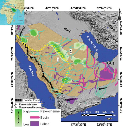
Locally, a few previous studies have delineated fluvial channels and mega-basins over regional scales using remote sensing and GIS. Dabbagh, Al-Hinai, and Khan (1997) used the SIR-C images to map some fluvial channel pathways in the Jafurah sand sea and Al-Labbah Plateau, Saudi Arabia (Figure 1), ancient lake beds (e.g., Clark 1989), and fluvial channels revealed by SIR-C images. These studies were based on visual interpretation and screen digitizing, which introduced a bias. In addition, none of these studies attempted to map the topographic index over a regional scale. Here, we present the first fluvial channels and mega-basins mapping from a SRTM DEM using the deterministic eight node (D8) algorithm; we analyzed the spatial distribution of the fluvial channels. We also aimed at mapping the topographic wetness index (TWI) over a regional scale based on the spatial distribution of fluvial channels and mega-basin area.

Figure 1. Reference map showing the major fluvial channels palaeolakes mapped from SIR-C (e.g., Edgell 2006, Dabbagh, Al-Hinai, and Khan 1997), and aerial photographs (e.g., Clarck 1989). Black line highlights water divide and green polygons highlight the circular farms densities in the region. The yellow line divides the region into renewable and non-renewable groundwater zones. Features in the figure reproduced with kind permission from Springer and Business Media. For full color versions of the figures in this paper, please see the online version.

2. Study area

The Kingdom of Saudi Arabia lies between latitudes 15º 14′ 00″ N and 31º 1′ 52″ N and longitudes 36º 55′ 33″ and 52º 52′ 12″. It covers an area of approximately 2.15 million km², and it represents the largest country in the Arabian Peninsula (Figure 1). The study area is divided into the Arabian shield in the west and the continental shelf in the east and southeast. The Arabian shield is a rugged mountain range that consists of igneous and metamorphic rocks; it is known as the Assir Mountains (elevation: 5000 m) and the Hejaz Mountain (elevation: 4500 m). The continental shelf is a lowland and depression that consists largely of sedimentary rocks and includes the Nafud desert in the north and Err Rub Al Khali (Empty Quarter) in the south (Figure 2).

Figure 2. Geological map of the study area showing lithological units and structural geology control groundwater accumulation and quality.

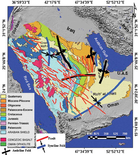
The major trends of the primary mountains in the region are mostly in the N34ºW direction and parallel the Najd fault zone; the other system (N8ºE) parallels the Hail Arc, and S89ºW parallels the central Arabian Arch (Figure 2). The bedrock geology in the region consists mainly of Quaternary sandstone (porous aquifer) underlain by carbonate rocks (karastifed fractured aquifer) (Clark 1989; Sharaf and Hussein 1996).

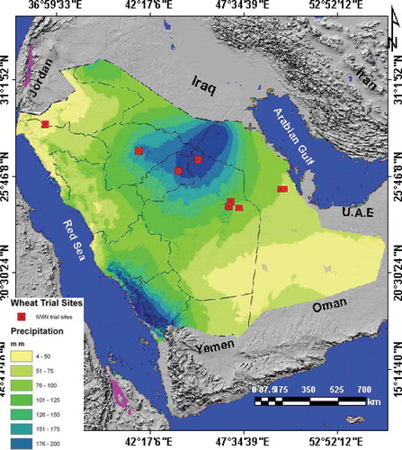
The climate is dominantly arid with a semi-arid climate along the Red Sea coast with an annual rainfall of approximately 52.5 mm between October and March, and a maximum rainfall of 284 mm occurring in 1996 (Subyani 2011) (Figure 3). The rainwater flows from the mountainous area to the lowlands and depressions in the east, northwest, southeast and Red Sea in the west; recharging the major aquifers in the region (Figure 1). The aquifers are recharged at a rate of approximately 2200 MCM/year, most of which goes to recharging shallow aquifers (Edgell 1997). The rate at which aquifers are recharged partially depends on topographic slope, the spatial distribution of fluvial channels (flow direction), fault intersections, and soil texture (Burdon 1982).

Figure 3. Rainfall map showing the spatial distribution of rainfall over the region. Red points highlight the International Wheat Improvement sites (IWIN).

According to the MAW (1984), the study area (Saudi Arabia) is characterized by six aquifers. These aquifers are locally known as Wajid sandstone, Saq sandstone, Tabuk (Tawil), Minjur sandstones, Wasia /Biyadh /Sakah sandstones and Umm Er Raduma limestone (Table 1). These aquifers are consolidated sedimentary rocks (sand stone and limestone) located in the eastern and central parts of the region known as the Arabian Shelf (Sharaf and Hussein 1996). According to the Water Atlas of Saudi Arabia, there are 253,000 MCM of proven reserves with estimates of up 700 billion cubic meter groundwater reserves (Table 1).

Table 1. Major fossil water aquifers in Saudi Arabia.

Aquifer	Storage (MCM	Available (MCM)	Area (km^2)	Outcrop area (km^2)	Thickness (m)	Fall in water table (1981–2002)	Comments
Saq sandstone	258,400	103,360	300,000	51,245	400–1200	16–76	Largest aquifer. High potential for development
Wajid sandstone	237,500	95,000	170,000	31,534	200–900	–	Only limited geological understanding
Tabuk (Tawil)	109,800	43920	~142,000	86,540	500–950	34	Upper unit of three sandstones separated by aquitards/aquicludes
Minjur sandstones	171,300	111,340	~48,000	29,648	400	80–85	The indicated surface area includes the Dhruma aquifer
Wasia/Biyadh/Sakah sandstones	66000	33,300		29,797	600	–	Largest system in the Kingdom after the Saq
Umm Er Raduma limestone	6000	3000		58,331	300–700	52–97	Lack of understanding of many physical parameters

Source: Country Report.

The Saq aquifer is the most valuable aquifer and occupies an area of approximately 300,000 km². It has the largest aerial extension and the most productive aquifer in the study area (Edgell 1997). The Saq aquifer has a thickness ranging from 150 to 500 m and an effective porosity exceeding 15% (Sharaf and Hussein 1996; Edgell 1997).

3. Data and pre-processing

3.1. Data sets

We used four remotely sensed data sets in this study. The first data were the new version of the SRTM DEM with a spatial resolution of 30 m. The original data of the SRTM (with a spatial resolution ~90 m) were acquired on 21 February 2000; an enhanced version of the data with a spatial resolution 30 m was released on 23 September 2014. We used the SRTM DEM to delineate near surface fluvial channels and mega-basins over the entire region. The second data included the SIR-C images with a spatial resolution of 25 m; these data were acquired on 10 October 1996. The data were used to compare the textural features (fluvial channels) evident from SRTM DEM and to determine whether these patterns were different. The SRTM sensor provides physical information about the depth and elevation of these features (McCauley et al. 1982; Paillou et al. 2009); while the SIR-C sensor has the ability to penetrate the dry sand sheets and image near-surface fluvial channels (Roth and Elachi 1975).

The third data were the Advanced Spaceborne Thermal Emission and Reflection Radiometer (ASTER) DEM with a spatial resolution of 30 m generated from optical data. These data were acquired on 11 October 2011 and distributed as a geographic (long/lat) projection, with the WGS84 horizontal datum currently available from the Earth Remote Sensing Data Analysis Centre (ERSDAC) database (http://www.gdem.aster.ersdac.or.jp/search.jsp).

The fourth data consisted of Landsat 8 Level 1T images with 30-m spatial resolution acquired on 13 April 2013 (P150/r45). Landsat images for the Worldwide Reference System (WRS-2) with UTM projection 38N were downloaded from the USGS Earth Resources Observations and Science (EROS) Center using the Global Visualization Viewer (www.glovis.usgs.gov) portal.

3.2. Preprocessing

As part of the preprocessing, the SRTM DEM was enhanced by applying a mean filter to remove holes in the DEM; the SIR-C images were enhanced by applying the enhanced Lee filter to remove speckles (Elmahdy et al. 2011; Elmahdy and Mohamed 2015c). The enhanced Lee filter filters remote sensing data based on statistics calculated using 3 × 3 individual filter windows (Eliason and McEwen 1990). We used these various data sets for visually comparing textural features (fluvial channels) evident in SRTM and determining spatial variations in the patterns of the SIR-C images (Elmahdy et al. 2012).

4. Methodology

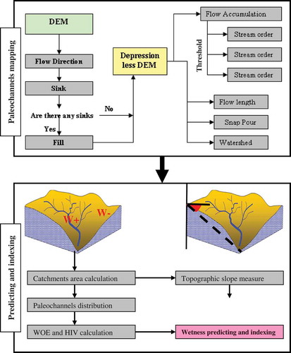
The proposed method can be divided into three steps: (i) regional mapping of near- surface fluvial channels and mega-basins and (ii) calculation of the TWI based on the calculated total area, topographic slope, and spatial distribution of the fluvial channels (Table 2), and (iii) validating the mapped features by comparing their textural features (fluvial channels) evident on the Imagine Radar (SIR-C) and Landsat 8 images and determining whether these textural features are different. We also validated the features mapped using the proposed method, which also validated by comparing them with previous maps of Clark (1989) and Dabbagh, Al-Hinai, and Khan (1997).

Table 2. Fluvial channel and mega-basin weights and information values (IVs). These fluvial channel have positive association to the topographic wetness and are, therefore, enhancing the predictive power. Mega-basins that have negative or no association to the spatial distribution of palaeochannels are shown in brackets (*).

	Mega-basins	Area (km^2)	Area (%)	Stream area (km^2)	Stream area (%)	Distribution good (DG)	Non-stream area (km^2)	Non-stream area (%)	Distribution bad (DB)	WOE	C = DG − DB	IV = C*WOE	Predictive power
1	Ar Rub Al Kali	93,172	4.86	28,657	30.75	0.17	64,515	69.25	0.03	1.73	0.14	0.2422	Very strong
2	Ad Dawasir	539,293	28.13	20,267	3.75	0.12	519,026	96.25	0.29	−1.23	−0.17	0.2091	Strong
3	Sahba	233,584	12.18	37,263	15.95	0.22	196,321	84.05	0.11	0.69	0.11	0.0759	Medium
4	Asulb	211,796	11.04	32,770	15.47	0.19	179,026	84.53	0.10	0.64	0.09	0.0576	Medium
5	Arrimah	226,081	11.79	12,041	5.32	0.07	214,040	94.68	0.12	−0.53	−0.05	0.0265	Medium
6	Nafud	153,934	8.03	9421	6.12	0.05	144,513	93.88	0.08	−0.47	−0.03	0.0141	Weak
7	Tabuk	181,393	9.46	8389	4.62	0.05	171,589	95.36	0.09	−0.58	−0.04	0.0232	Medium
8	Arran	121,743	6.35	6272	5.15	0.03	115,471	94.85	0.06	−0.69	−0.03	0.0207	Medium
9	*Coastal basin	152,866	7.97	10,263	6.71	0.06	142,603	93.29	0.08	−0.28	−0.02	0.0056	Useless
	Total	1,913,862		165,343			1,747,104

Notes: distribution good = stream area/total stream area. Distribution bad = non stream area/total area.

Weight of evidence (WOE) = ln (distribution good/distribution bad). *Coastal basin.

The primary advantages of the proposed methods are:

(i) it permits assigning a weight to the statistical association between the fluvial channels and the total area of the mega-basins;

(ii) it directly displays the spatial relationship between the spatial distribution of the fluvial channels and the TWI;

(iii) it is time and cost effective for a regional mapping in remote and inaccessible areas.

4.1. Regional mapping of the near-surface fluvial channels and mega-basins

To map the major fluvial channels and mega-basins over regional scales, it is important to employ an automated algorithm. We used the D8 algorithm of Jenson and Domingue (1988), which is implemented in ArcGIS v. 9.2 software, to map fluvial channels beneath sand sheets. As a first step, the algorithm was applied separately to two grids of SRTM DEM with a spatial resolution of 30 m to ASTER DEM of spatial resolution of 30 m. The D8 algorithm, which determines in which neighboring pixel any water in a central pixel will flow naturally, was used to delineate fluvial channels and mega-basins in the study area.

The algorithm consists of three steps: (i) filling in the pits (no data) in the DEM and then determining which neighboring pixel water in a central pixel will flow naturally, (ii) incorporating the flow direction to determine the most likely flow paths for drainage over the given DEM, (iii) defining a threshold definition (stream definition). Threshold definition (stream definition) was performed by training several threshold values ranging from 1000 to 10,000 on SRTM and ASTER DEMs. We mapped fluvial channels and mega-basins using the hydrology tool implemented in the ArcGIS software.

To assess the accuracy of the mapped fluvial channels, we used two methods. In the first method, we compared the patterns of fluvial channels with those mapped from SIR-C images by Dabbagh, Al-Hinai, and Khan (1997) and lakes discovered by Clark (1989) (Figure 1). In the second method, we correlated the fluvial channels by comparing the textural features evident from SRTM DEM and SIR-C and determined whether these patterns were different (Elmahdy and Mohamed 2013, 2015c).

4.2. Spatial analysis

The spatial distribution and length of the fluvial channels and the total area of each mega-basin were counted and recorded in Table 2 for calculating of the channel frequency (Cf) and fluvial channel density (Cd). The fluvial channel frequency can be defined as the total number of streams divided by the total area of the basin. The fluvial channel density can be defined as the total length of all streams in a basin divided by its total area; this quantity reflects potential for runoff and infiltration. Fluvial channel frequency and density in each mega-basin were calculated in represented in maps using quantitative tools implemented in the ArcGIS v.9.2 software.

4.3. Weight of evidence (WOE) and its application

4.3.1. Theory of WOE

The WOE is a geo-statistical, predictive method proposed by Agterberg et al. (1993). The WOE was originally developed for medical diagnostics (Lusted 1968; Aspinall and Hill 1983).

The WOE combines different data sets, as controlling factors of the occurrence of a particular phenomenon by weighting each factor using a long linear from a Bayesian- based model (Sawatzky et al. 2009).

Suppose that the jth binary map is Bj, D refers to the presence of deposits and the positive WOE (W+) is defined as (Bonham-Carter, Agterberg, and Wright 1989; Agterberg et al. 1993)

(1)

The negative WOE (W^–) is defined as (Bonham-Carter, Agterberg, and Wright 1989; Agterberg et al. 1993)

(2)

where P(Bj/D) is the conditional probability of the presence of the jth binary map giving the presence of a deposit, P(Bj/D′) is the conditional probability of the presence of the jth binary map giving the absence of a deposit; P(Bj′/D) is the conditional probability of the absence of the jth binary map giving the presence of a deposit and P (Bj′/D′) is the conditional probability of the absence of the jth binary map giving the absence of a deposit. The contrast Cj for the jth map is an overall measure of the spatial association between the deposits and the binary pattern (Bonham-Carter, Agterberg, and Wright 1989; Agterberg et al. 1993):

(3)

and, the variance of the weights, s(Cj), for the jth map is defined as (Bonham-Carter, Agterberg, and Wright 1989; Agterberg et al. 1993)

(4)

Cj > 0 if the spatial association is positive, Cj < 0 if the spatial association is negative, and Cj = 0 if there is no spatial association. Sometimes, Cj, particularly with a small number of deposits, has no significant larger value and no significance (Carranza and Hale 2000); however, studentized contrast, Stud (Cj), as the ratio of the contrast to its standard deviation, Cj/s (Cj), provides a more reliable measure of spatial correlation (Bonham-Carter 1994).

4.3.2. Application

The usage of WOE has spread into other fields, such as predicting the sites of mineral ore (Bonham-Carter, Agterberg, and Wright 1989; Agterberg et al. 1993; Bonham-Carter 1994; Carranza and Hale 2000), landslide susceptibility mapping (Luzi, Pergalani, and Terlien 2000), and ground subsidence hazard mapping (Dahal et al. 2008). However, none of these studies have been applied to map and calculating regional TWI using IV, which is a modified version of the WOE model.

Applying the IV model to map TWI involves the following steps:

1. Selecting a set of significant hydrological parameters that are useful for evidential themes for the TWI. These parameters may involve maps of fluvial channels and mega-basins.

2. For each mega-basin, the total area of the fluvial channels was calculated to determine good (GD) and bad distributions (BD).

3. Calculating the WOE for each mega-basin as the logarithmic ratio of the GD and the BD using Equation (5).

   (5)

4. The overall level of spatial association between the GD and BD is given by the parameters of contrast, C, which is defined by Equation (6).

   (6)

5. Calculating the IV by multiplying the C and WOE using Equations (7) and (8).

   (7)
   (8)

According to Zeng (2014), by convention the values of the IV statistic can be interpreted as follows.

If the IV statistic is:

1. Less than 0.01 then the predictor is not useful for modeling (separating the DG from the DB).

2. 0.01–0.1 then the predictor has only a weak relationship with the DG/DB odds ratio.

3. 0.1–0.2, then the predictor has a medium strength relationship with the DG/DB odds ratio

4. 0.2 or higher, then the predictor has a strong relationship with the DG/DB odds ratio.

The implementation steps of IV are summarized in Figure 4 and Table 2.

Figure 4. Flow chart of the methodology used for mapping fluvial channels and indexing topographic wetness. W+ and W– highlight the areas of good and bad fluvial channels distribution, respectively.

4.4. TWI and its application in regional mapping

We carried out TWI mapping in the following way. First, we calculated the total area of each mega-basin. Next, we measured the topographic slope of each mega-basin from the highest point to the lowest point using a line of sight tool implemented in the open source Microdem v. 12 software (Guth 2006). We calculated the mega-basin area and topographic slope using the following equation:

(9)

where a represents the mega-basin area and ß refers to the topographic slope.

When the TWI value exceeds 16, the predictive power of the model becomes higher. On the contrary, TWI value less than 10 indicates low predictive power.

Figure 4 and Table 3 summarize the procedures implemented to map TWI.

Table 3. Predictive soil wetness values of each mega-basin in the region.

No.	Mega-basins	Catchments area (a)	Topographic slope angle (β) (°)	Topographic wetness TWI = ln (a/β)	Predictive power
1	Rub Al Kali	28,657	0.01	14	High
2	Ad Dawasir	20,267	0.11	16.7	Very high
3	Sahba	37,263	0.07	13.18	High
4	Asulb	32,770	0.16	12.22	Medium
5	Arrimah	12,041	0.07	12	Medium
6	Nafud	9421	0.08	11.67	Medium
7	Tabuk	8389	0.10	11.33	Low
8	Arran	6272	0.23	10.21	Low
9	Coastal basin	10,263	0.70	9.60	Very low
	Total	165,343

5. Results

5.1. Mapping of mega-basins and fluvial channels

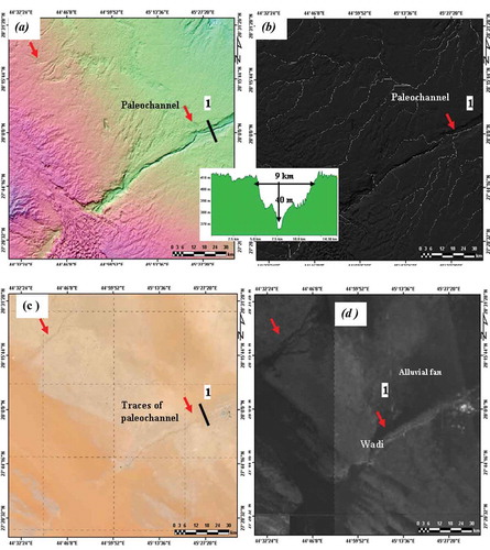
We modified the D8 algorithm by selecting a suitable threshold value for mapping the regional fluvial channels beneath sand sheets. The new maps of fluvial channels and mega-basins revealed from DEM using the D8 algorithm are shown in Figure 5. The maps show that the region is characterized by nine tributaries mainly drain from the Assir, Hegaz and Oman mountains terminating at Err Rub Al Khali, Ad Dawasir, Sahba, Asulb, Arrimah, Nafud, Tabuk, Arran, and to the Red Sea in the west and the Arabian Gulf in the east southeast. These features were formed by fluvial process during the late Quaternary (Clark 1989). The tributaries, which are 74–472 km in length, flow under the influence of slope and the NNW–SSE and NW–SE trending faults that are displaced 40-m depth and have length of more than 9 km [Figures 3, 5, 6(a) and 6(b)].

Figure 5. Fluvial channel and mega-basin maps derived from SRTM DEM using D8 algorithm (a), and ENE–WSW topographic profile across the Saudi Arabia, showing flow direction and flow type in the region.

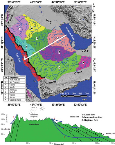
Figure 6. Zooms of fluvial channels derived from DEM using a D8 algorithm (a and b), from the corresponding Landsat 8 (c), and SIR-C image (d), showing detail of fluvial channels (wadis) on SRTM DEM, traces on Landsat 8 image, and fluvial fans on SIR-C image. These show the capability of the SRTM and SIR-C SAR sensors to imagine details of fluvial channels than optical sensors.

The tributaries are dendritic in shape in the coastal area and longitudinal in shape at the continental shelf, reflecting the topographic slope.

The dendritic fluvial channels reflect terrain with a steep slope, and the longitudinal fluvial channels reflect terrain with very gentle slope. In terrain with a very gentle slope, surface water decelerates and the infiltration rate increases. These currently dry valleys can occasionally be flooded as shown in rainfall maps (MAW 2003). These fluvial channels are made up alluvial fans and shallow aquifers, which represents the primary source of renewable groundwater and fossil water of deep aquifers (Clark 1989).

An original approach combining multi-sources of remote sensing data provided new evidence for the existence of regional fluvial channels and Err Rub Al Khali Lake, as confirmed visually by Landsat 8 and SIR-C images [Figure 6(c) and 6(d)], and comparable studies (Clark 1989; Dabbagh, Al-Hinai, and Khan 1997). This lake receives a considerable amount of water from the Oman mountains in the east and southeast and Hegaz mountain in the west and southwest. This lake is characterized by lakebeds of pure calcium carbonate and gypsum that stand out in stark white from the reset of the desert in Landsat images (Clark 1989; Dabbagh, Al-Hinai, and Khan 1997). These deposits are often indicative of a closed basin’s environment (maco-depression) with a very gentle slope and may represent sites with groundwater potential (Clark 1989).

5.2. Spatial analysis

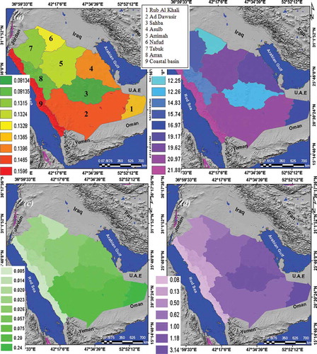
The fluvial channel patterns mapped from the SRTM DEM are mostly longitudinal in the continental shelf (east and southeast) and dendritic in the coastal area (west). We carried out a spatial analysis of fluvial channel patterns based on the fluvial channels frequency (Cf) and the fluvial channels density (Cd). The values of these parameters are shown in Figure 7(a) and 7(b). The highest values of Cf and Cd (0.1596 and 21.88) in Ad Dawasir and the coastal mega-basin; the lowest values (0.018 and 12.25) were recorded at the Sahba and Nafud mega-basins.

Figure 7. Maps of fluvial channel distribution (a), fluvial channel density (b), IV (c), and topographic wetness index (TWI) (d), showing the influence of the spatial distribution of palaeochnnels and slope on the topographic wetness in the entire region sensors.

According to Mohamed and Elmahdy (2015), a higher value frequency and density of fluvial channels fluvial channel reflects a steep slope and thin regolith; a low fluvial channel frequency and density are indicative of a gentle slope and thick regolith. Areas underlain by a thick regolith are important from a hydrogeological point of view because this deposition confers a high degree of water-storage capacity (Tennakon 1989).

5.3. Mapping of topographic wetness

The maps constructed based on IV and WOE values are shown in Figure 7(c), and the productive power values are summarized in Table 2. This table lists different classes of predictive power based on IV values. For example, a very strong predictive power class has a value greater than 0.2, a strong predictive power class has a value equal to 0.2, a medium predictive power class has a value greater than 0.1, a weak predictive power class has a value less than 0.01, and a useless predictive power class has value less 0.001. Err Rub Al Khali and Ad Dawasir, which occupy an area of 632.46 km², have the highest predictive power values. These mega-basins also occupy one third of the total study area (Table 2). The data in Table 2 reveal that there is a small difference between wetness indices using WOE and IV and TWI. The IV value is the highest in the continental shelf in the east, and the IV value is the lowest in the Arabian shield and coastal mega-basin in the west.

The TWI map calculated based on the topographic slope and catchment area is shown in Figure 7(d). The map shows that the Err Rub Al Khali and Sahba mega-basins have the highest value of TWI (>3), and that the Arran and coastal mega-basins have the lowest value of TWI (<0.08). As a result of WOE, IV, and TWI analyses, a larger distribution of fluvial channels, a gentler slope and a larger mega-basin area are indicative of groundwater potentiality. The TWI reveals a strong agreement between IV and groundwater predictive power (Figure 7(c), 7(d) and Table 2).

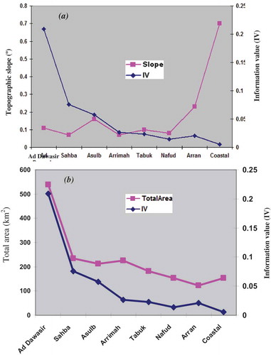
The spatial relationships among topographic slope, groundwater mega-basin area and IV are shown in Figure 8. For terrain with a very gentle slope, surface water decelerates and the infiltration rate increases; the probability of groundwater accumulation accordingly increases. In total, the maximum IV and the significant slope are below 1º [Figure 8(a)]. We concluded a similar analysis of the IV is done with every mega-basin [Figure 8(b)]. As the area of the mega-basin increases, the IV increases; therefore, the probability of groundwater accumulation increases as well.

Figure 8. Graphs of topographic slope vis IV (a) and mega-basin area vis IV (b).

The resulting maps were validated using fluvial channels mapped from SIR-C images by Dabbagh, Al-Hinai, and Khan (1997) and lakes discovered by Clark (1989). This validation involved comparing the textural features evident from SRTM and Landsat 8 and SIR-C and determining whether these patterns were different. We found a strong agreement between the mapped fluvial channels from SRTM DEM and those mapped from SIR-C and Landsat 8 images (Figures 1 and 6). We accordingly recovered a good correspondence between areas of the highest values of TWI and IV, and the discovered lakes (Clark 1989; Dabbagh, Al-Hinai, and Khan 1997), and the depression of Err Rub Al Khali (Figures 1 and 7). This finding supports the suggestion that the depression of Err Rub Al Khali (Ad Dawasir and Umm As Samim) is possibly the largest accumulation of sand and surface and fossil water in the region because it receives water from two rechargeable areas (the Oman and Hejaz mountains).

6. Discussion

Several studies have mapped palaeochannels using the D8 algorithm from the SRTM DEM with a spatial resolution of 90 m and radar images (McCauley et al. 1982; Paillou et al. 2009; Elmahdy and Mohamed 2013, 2014a). However, these studies were based on only mapping palaeochannels and mega-basins; none of these studies attempted to estimate and calculate the regional TWI. As a result, the regional hydrological setting of the Saudi Arabia remains largely unexplored and poorly understood.

The D8 algorithm, which uses a DEM, was modified by selecting a suitable threshold value for delineating the regional fluvial channels. The algorithm performed well at delineating near-surface fluvial channels and mega-basins in arid and semi-arid regions. The Landsat and SIR-C images and ASTER DEM confirm the presence of fluvial channels beneath the sand sheet. Furthermore, the palaeochannels mapped from SIR-C images and given in the literature (e.g., Clark 1989; Dabbagh, Al-Hinai, and Khan 1997) were largely met.

The SRTM data exhibited a better vertical accuracy and more detail and a smaller number of artifacts than the ASTER GDEM data (Fujisada et al. 2005; Elmahdy et al. 2012). It is also important to note that the D8 algorithm worked well on the SRTM DEM and showed much more detail than the ASTER GDEM data with a spatial resolution of 30 m. Furthermore, the Landsat 8 sensors demonstrated its ability to discriminate the spectral signature of fluvial channels filled in with fluvial deposits. This signature, which appears as linear dark and/or light tones, proves that near surface features cannot be mapped using optical remote sensing data (Paillou et al. 2009).

The SRTM and SIR-C sensors exhibited a powerful ability to penetrate dry sand sheets and image near-surface geological and hydrological features in a time-and cost-effective manner (Elmahdy et al. 2011; Elmahdy and Mohamed 2014a; Elmahdy, Mohamed, and Marghany 2014; Elmahdy and Mohamed 2015b, 2015c). The result of the new version of SRTM DEM processing revealed that the Saudi Arabia is drained by nine tributaries. These tributaries drain from the Asir, Hegaz, and Oman mountains to terminate at Err Rub Al Khali, Ad Dawasir, Sahba, Asulb, Arrimah, Nafud, Tabuk, Arran and the Red Sea in the west and the Arabian Gulf in the east southeast. Hydrological parameters such as fluvial channels and mega-basins were considered to be significant. The spatial distribution of fluvial channels and the total area of mega-basins were used to calculate the predictive power (TWI) for each mega-basin. For example, the DG of fluvial channels and mega-basin area had a positive relationship with the TWI. This index supports the suggestion that the depression of Err Rub Al Khali (Ad Dawasir and Umm As Samim) was possibly represents the largest accumulation of sand surface and fossil water in the region because it receives water from two sources that are rechargeable areas (the Oman and Hejaz mountains).

The TWI calculated using the IV model showed that Err Rub Al Khali and Sahba are the wettest mega-basins in the Saudi Arabia and that these regions may have received a considerable amount of fossil water during the Late Quaternary. During this period, the entire region was considerably wetter than it is today based on lakebed data (e.g., Clark 1989), and palaeochannel data (Dabbagh, Al-Hinai, and Khan 1997). We recovered strong agreement between the mapped fluvial channels from the SRTM DEM and those mapped from SIR-C and Landsat images (Figures 1 and 6). In other words, the SRTM DEM and Landsat in corporation with SIR-C support the presence of near-surface fluvial channels beneath the sand sheet.

Automated algorithms such as the D8 algorithm are useful for regional mapping of fluvial channels and mega-basins in arid and semi-arid regions. As a result of our IV and WOE analysis, we found that a higher spatial distribution of fluvial channels and a lower topographic slope may produce a higher infiltration and accordingly more groundwater production. Our findings indicate a clear spatial association among the mega-basin area, and topographic slope and IV; these trends likewise suggest a link to groundwater productivity.

Fluvial channels and catchments are good hydrological indicators of areas of groundwater accumulation. We accordingly integrated remote sensing and IV in a GIS environment to map fluvial channels and mega-basins and analyze their spatial distribution in terms of TWI over a regional scale. The present approach was used to enhance the performance of each individual TWI method. The combined use of active data (such as SRTM DEM) and optical data (Landsat 8 images) proved successful at delineating fluvial channels and led to a better understanding of Saudi Arabia’s hydrological setting. The IV model offers the transparency in its calculation of the weights and enables time- and cost-effective investigations of significant factors, such as the spatial distribution of fluvial channels, mega-basins, and topographic slope.

7. Conclusion

Thus far, a limited number of studies have been conducted to map fluvial channels and TWI over regional scales in Saudi Arabia. With the aid of remote sensing data and IV in GIS, we have provided complete fluvial channel and TWI maps over regional scales in Saudi Arabia for the first time. These hydrological features, in conjunction with the topographic slope, were used as input parameters for developing methods to map and predict TWI over a regional scale. Our results revealed that Err Rub Al Khali and Ad Dawasir have the highest IV and TWI values; these sites are accordingly associated with of a higher likelihood of harboring groundwater. Integration of various near-surface hydrological indicators that control groundwater accumulation is an essential aspect in water resources and groundwater exploration studies. Our maps will be of significant aid to hydrologists in choosing sites for groundwater exploration. Our investigation has enhanced our understanding of the regional hydrological setting of the Saudi Arabia. This study is the prerequisite for bridging the gap between research and operational methods for TWI remote sensing. This study has allowed different sensors and algorithms to be compared across arid and semi-arid regions.

Acknowledgments

The authors acknowledge the assistance provided by UAE National Water Center (NWC) and the UAE University Program for Advanced Research (UPAR).

Disclosure statement

No potential conflict of interest was reported by the authors.

Additional information

Funding

This research was supported by funds from the UAE National Water Center (NWC) and the UAE University Program for Advanced Research (UPAR) [projects numbers NWC-3-2013-31R008 and UPAR-7-2013-31N166].

References

- Agterberg, F. P., G. F. Bonham-Carter, Q. Cheng, and D. Wright. 1993. “Weights of Evidence Modeling and Weighted Logistic Regression for Mineral Potential Mapping.” Computers in Geology 25: 13–32. Oxford University Press.
- Aspinall, P., and A. R. Hill. 1983. “Clinical Inferences and Decisions E I. Diagnosis and Bayes’ Theorem.” Ophthalmic & Physiological Optics 3: 295–304.
- Bhang, K. J., and F. W. Schwartz. 2008. “Limitations in the Hydrologic Applications of C-Band SRTM DEMs in Low-Relief Settings.” IEEE Geoscience and Remote Sensing Letters 5: 497–501. doi:10.1109/LGRS.2008.920712.
- Bhang, K. J., F. W. Schwartz, and A. Braun. 2007. “Verification of the Vertical Error in C Band SRTM DEM Using ICESat and Landsat-7, Otter Tail County, MN.” IEEE Transactions on Geoscience and Remote Sensing 45: 36–44. doi:10.1109/TGRS.2006.885401.
- Bonham-Carter, G. F. 1994. Geographic Information Systems for Geoscientists, Modeling with GIS. Oxford: Pergamon Press.
- Bonham-Carter, G. F., F. P. Agterberg, and D. F. Wright. 1989. “Weights of Evidence Modeling: A New Approach to Mapping Mineral Potential.” Statistical Applications in the Earth Sciences 89: 171–183.
- Burdon, D. J. 1982. “Hydrogeological Conditions in the Middle East.” Quarterly Journal of Engineering Geology and Hydrogeology 15: 71–82. doi:10.1144/GSL.QJEG.1982.015.02.01.
- Carranza, E. J. M., and M. Hale. 2000. “Geologically Constrained Probabilistic Mapping of Gold Potential, Baguio District, Philippines.” Natural Resources Research 9: 237–253. doi:10.1023/A:1010147818806.
- Clark, A. 1989. “Lakes of the Rub’ Al-Khali.” Aramco World 40 (3): 28–33.
- Dabbagh, A. E., K. G. Al-Hinai, and M. A. Khan. 1997. “Detection of Sand-Covered Geologic Features in the Arabian Peninsula Using SIR-C/X-SAR Data.” Remote Sensing of Environment 59 (2): 375–382. doi:10.1016/S0034-4257(96)00160-5.
- Dahal, R. K., S. Hasegawa, A. Nonomura, M. Yamanaka, T. Masuda, and K. Nishino. 2008. “GIS-Based Weights-Of-Evidence Modelling of Rainfall-Induced Landslides in Small Catchments for Landslide Susceptibility Mapping.” Environmental Geology 54: 311–324. doi:10.1007/s00254-007-0818-3.
- Doll, P., B. Lehner, and F. Kaspar. 2002. “Global Modeling of Groundwater Recharge.” In Proceedings of 3rd International Conference on Water Resources and the Environment Research, Vol. 1, 27–33. Dresden: Technical University of Dresden.
- Edgell, H. S. 1997. “Aquifers of Saudi Arabia and Their Geological Framework.” Arabian Journal of Science and Engineering 22 (1C): 3–32.
- Elachi, C., L. E. Roth, and G. Schaber. 1984. “Spaceborne Radar Subsurface Imaging in Hyperarid Regions.” IEEE Transactions on Geoscience and Remote Sensing 22: 383–388. doi:10.1109/TGRS.1984.350641.
- Eliason, E. M., and A. S. McEwen. 1990. “Adaptive Box Filters for Removal of Random Noise from Digital Images.” Photogrammetric Engineering & Remote Sensing 56 (4): 453.
- Elmahdy, S. I., S. Mansor, B. B. K. Huat, and A. R. Mahmod. 2012. “Structural Geologic Control with the Limestone Bedrock Associated with Piling Problems Using Remote Sensing and GIS: A Modified Geomorphological Method.” Environmental Earth Sciences 66 (8): 2185–2195. doi:10.1007/s12665-011-1440-y.
- Elmahdy, S. I., S. Mansor, A. Rodsi, and B. K. Bujang. 2011. “Geotechnical Modeling of Fractures and Cavities that are Associated with Geotechnical Engineering Problems in Kuala Lumpur Limestone, Malaysia.” Environmental Earth Sciences 62 (1): 61–68. doi:10.1007/s12665-010-0497-3.
- Elmahdy, S. I., M. M. Mohamed, and M. M. Marghany. 2014. “Mapping and Classification of Hydrological Parameters from Digital Terrain Data in the Musandam Peninsula, UAE and Oman.” Geocarto International 1–16. doi:10.1080/10106049.2014.883433.
- Elmahdy, S. I., and M. M. Mohamed. 2013. “Remote Sensing and GIS Applications of Surface and Near-Surface Hydromorphological Features in Darfur Region, Sudan.” International Journal of Remote Sensing 34 (13): 4715–4735. doi:10.1080/01431161.2013.781287.
- Elmahdy, S. I., and M. M. Mohamed. 2014b. “Groundwater Potential Modelling Using Remote Sensing and GIS: A Case Study of the Al Dhaid Area, United Arab Emirates.” Geocarto International 29 (4): 433–450.
- Elmahdy, S. I., and M. M. Mohamed. 2014a. “Automatic Detection of near Surface Geological and Hydrological Features and Investigating Their Influence on Groundwater Accumulation and Salinity in Southwest Egypt Using Remote Sensing and GIS.” Geocarto International 1–13. doi:10.1080/10106049.2014.883433.
- Elmahdy, S. I., and M. M. Mohamed. 2015a. “Probabilistic Frequency Ratio Model for Groundwater Potential Mapping in Al Jaww Plain, UAE.” Arabian Journal of Geosciences 8 (4): 2405–2416.
- Elmahdy, S. I., and M. M. Mohamed. 2015b. “Mapping of Tecto-Lineaments and Investigate Their Association with Earthquakes in Egypt: A Hybrid Approach Using Remote Sensing Data.” Geomatics, Natural Hazards and Risk 1–20.
- Elmahdy, S. I., and M. M. Mohamed. 2015c. “Groundwater of Abu Dhabi Emirate: A Regional Assessment by Means of Remote Sensing and Geographic Information System.” Arabian Journal of Geosciences 8 (12): 11279–11292.
- Elmahdy, S. I., and M. M. Mostafa. 2013. “Natural Hazards Susceptibility Mapping in Kuala Lumpur, Malaysia: An Assessment Using Remote Sensing and Geographic Information System (GIS).” Geomatics, Natural Hazards and Risk 4 (1): 71–91. doi:10.1080/19475705.2012.690782.
- Esteban, R., R. John, and S. Laura. 2013. “Mapping Forest Damage in Northern Nicaragua after Hurricane Felix (2007) Using MODIS Enhanced Vegetation Index Data.” GIScience & Remote Sensing 50 (4): 385–399.
- Farr, T. G., P. A. Rosen, E. Caro, R. Crippen, R. Duren, S. Hensley, and D. Seal. 2007. “The Shuttle Radar Topography Mission.” Reviews of Geophysics 45 (2). doi:10.1029/2005RG000183.
- Fujisada. H., G. B. Bailey, G. G. Kelly, S. Hara, and M. J. Abrams. 2005. “ASTER DEM Performance.” IEEE Transactions on Geoscience and Remote Sensing 43 (12): 2707–2714. doi:10.1109/TGRS.2005.847924.
- Guth, P. L. 2006. “Geomorphometry from SRTM: Comparison to NED: Photogrammetric Engineering & Remote Sensing.” Special issue based on Shuttle Radar Topography Mission—Data Validation and Applications Workshop, Reston, VA, 14 June 2005, 72 (3): 269–277.
- Jenson, S., and J. Domingue. 1988. “Extracting Topographic Structure From Digital Elevation Model Data for Geographic Information System Analysis.” Photogrammetric Engineering and Remote Sensing 54: 1593–1600.
- Loveson, V. J., K. Richa, M. Sundararajan, and A. R. Gujar. 2014. “Remote-Sensing Perspective and GPR Subsurface Perception on the Growth of a Recently Emerged Spit at Talashil Coast, West Coast of India.” GIScience & Remote Sensing 51 (6): 644–661. doi:10.1080/15481603.2014.972865.
- Lusted, L. B. 1968. Introduction to Medical Decision Making. Springfield, IL: Charles Thomas.
- Luzi, L., F. Pergalani, and M. T. J. Terlien. 2000. “Slope Vulnerability to Earthquakes at Subregional Scale, Using Probabilistic Techniques and Geographic Information Systems.” Engineering Geology 58: 313–336. doi:10.1016/S0013-7952(00)00041-7.
- MAW (Ministry of Agriculture and Water). 1984. Water Atlas of Saudi Arabia. Riyadh.
- Ministry of Agriculture and Water (MAW) 2003. Water Atlas of Saudi Arabia. Riyadh.
- McCauley, J. G., C. Schaber, C. Breed, V. Haynes, J. Grolier, B. Issawi, C. Elaichi, and R. Blom. 1982. “Subsurface Valleys and Geoarchaeology of Egypt and Sudan Revealed by Radar.” Science 218: 1004–1020. doi:10.1126/science.218.4576.1004.
- Mohamed, M. M., and S. I. Elmahdy. 2015. “Natural and Anthropogenic Factors Affecting Groundwater Quality in the Eastern Region of the United Arab Emirates.” Arabian Journal of Geosciences 8 (9): 7409–7423.
- Nyarko, B. K., B. Diekkrüger, N. C. Van De Giesen, and P. L. G. Vlek. 2015. “Floodplain Wetland Mapping in the White Volta River Basin of Ghana.” GIScience & Remote Sensing 52 (3): 374–395. doi:10.1080/15481603.2015.1026555.
- Paillou, P. M., M. Schuster, S. Tooth, T. Farr, A. Rosenqvist, S. Lopez, and J.-M. Malezieux. 2009. “Mapping of a Major Paleodrainage System in Eastern Libya Using Orbital Imaging Radar: The Kufrah River.” Earth Planetary Science Letters 277: 327–333. doi:10.1016/j.epsl.2008.10.029.
- Powers, R. P., N. C. Coops, J. L. Morgan, M. A. Wulder, T. A. Nelson, C. R. Drever, and S. G. Cumming. 2013. “A Remote Sensing Approach to Biodiversity Assessment and Regionalization of the Canadian Boreal Forest.” Progress in Physical Geography 37 (1): 36–62. doi:10.1177/0309133312457405.
- Roth, L. E., and C. Elachi. 1975. “Coherent Electromagnetic Losses by Scattering from Volume Inhomogeneities.” IEEE Transactions on Antennas and Propagation 23: 674.
- Sawatzky, D. L., G. L. Raines, G. F. Bonham-Carter, and C. G. Looney 2009. Spatial Data Modeller (SDM): ArcMAP 9.3 geoprocessing tools for spatial data modelling using weights of evidence, logistic regression, fuzzy logic and neural networks. http://arcscripts.esri.com/details.asp?dbid=15341
- Sharaf, M. A., and M. T. Hussein. 1996. “Groundwater Quality in the Saq Aquifer, Saudi Arabia.” Hydrological Sciences Journal 41 (5): 683–696. doi:10.1080/02626669609491539.
- Srinivasa Rao, Y., and D. K. Jugran. 2003. “Delineation of Groundwater Potential Zones and Zones of Groundwater Quality Suitable for Domestic Purposes Using Remote Sensing and GIS.” Hydrological Sciences Journal 48: 821–833. doi:10.1623/hysj.48.5.821.51452.
- Subyani, A. M. 2011. “Hydrologic Behaviour and Flood Probability for Selected Arid Basins in Makkah Area.” Western Saudi Arabia, Saudi Society for Geosciences 4 (5–6): 817–824.
- Tennakon, T. M. T. B. 1989. “The Study of the Relationship between Well Yields and Relevant Hydrogeological Phenomenon in Crystalline Basement Rocks in Northwestern Dry Zone of Sri Lanka.” Proceedings of the Groundwater Exploration and Development in Crystalline Basement Aquifers, Zimbabwe 2: 235–247.
- Wang, X., N. Chen, Z. Chen, X. Yang, and J. Li. 2016. “Earth Observation Metadata Ontology Model for Spatiotemporal-Spectral Semantic-Enhanced Satellite Observation Discovery: A Case Study of Soil Moisture Monitoring.” GIScience & Remote Sensing 53 (1): 22–44.
- Zeng, G. 2014. “A Necessary Condition for a Good Binning Algorithm in Credit Scoring.” Applied Mathematical Sciences 8 (65): 3229–3242.