Application of Aqua MODIS sensor data for estimating chlorophyll a in the turbid Case 2 waters of Lake Erie using bio-optical models

Abstract

There is considerable interest in accurately estimating water quality parameters in turbid (Case 2) and eutrophic waters such as the Western Basin of Lake Erie (WBLE). Lake Erie is a large, open freshwater body that supports diverse ecosystem, and over 12 million people in the mid-western part of the United States depend on it for drinking water, fisheries, navigational, and recreational purposes. The increasing utilization of the freshwater has deteriorated the water severely and currently the lake is experiencing recurring harmful algal blooms (HABs). Improving the water quality of Lake Erie requires the use of robust monitoring tools that help water quality managers understand sources and pathways of influxes that trigger HABs. Satellite-based remote sensing sensor such as the moderate resolution imaging spectroradiometer (MODIS) may provide frequent and synoptic view of the water quality indices. In this study, data set from field measurements was used to evaluate the performance of 14 existing ocean color algorithms. Results indicated that MODIS data consistently underestimated the chlorophyll a concentrations in the WBLE, with the largest source of errors from dissolved organic matter and xanthophyll accessory pigments in this data set. Most of the global algorithms, including OC4v4 and the Baltic model, generated near-identical statistical parameters with an average R² of ~0.57 and RMSE ~2.9 μg/l. MODIS performed poorly (R² ~0.18) when its NIR/red bands were used. A slightly improved model was developed using similar band ratio approach generating R² of ~0.62 and RMSE ~1.8 μg/l.

Keywords:

• chlorophyll a
• MODIS
• Lake Erie
• remote sensing

Introduction

Lake Erie has experienced recurring eutrophication over the last four decades and, consequently, the ecosystem has continuously changed during that period (Conroy et al. 2005). Bloom magnitude has increased since the mid-1990s and in 2011, the Western Basin of Lake Erie (WBLE) experienced the largest algal bloom in its recorded history. Being the shallowest and southernmost Great Lake, Lake Erie has warm temperatures, which are conducive to biological productivity. The tendency toward excessive biological productivity, eutrophication, is exacerbated by the fluvial nutrient influx from agricultural runoff and combined sewer overflows. Some of the algal blooms are composed of species that produce toxins (e.g., Microcystis aeruginosa and Planktothrix spp.) or taste and odor problems (e.g., Cladophora) in the drinking water (Conroy et al. 2005). These toxic blooms can be detrimental and pose a threat to public safety.

Understanding and monitoring the impacts of environmental stresses on Lake Erie requires robust monitoring. Traditional water quality monitoring is conducted through analysis of water samples obtained from preselected sites. This method has greatly enhanced our understanding of the stressors and the resulting symptoms; however, this approach is generally insufficient to provide the spatial and temporal coverage needed to continuously assess water quality on basin-wide scales in large, open water bodies such as Lake Erie. Satellite remote sensing provides complementary information and has the potential to greatly improve our understanding of variations in water quality.

Satellite imaging systems that detect variations in spectral reflectance from the Earth’s surface are promising for evaluating water quality in large, open water bodies (Baban 1995; D’Sa 2014; De Cauwer et al. 2004; El-Alem et al. 2012; Gons 1999; Nellis, Harrington, and Wu 1998; Ouillon, Douillet, and Andréfouët 2004; Schmugge et al. 2002; Shuchman et al. 2006; Simis, Peters, and Gons 2005; Tarrant and Neuer 2009; Torbick et al. 2008). These assessments are made by applying algorithms that relate satellite-measured reflectance (color) to the concentration of specific water quality constituents, e.g., chlorophyll a (see Martin 2004). Chlorophyll a is the dominant light-harvesting pigment and is universally present in eukaryotic algae and the Cyanophyceae (cyanobacteria) (Rowan 1989). The pigment is commonly measured in water quality monitoring programs for coastal and inland waters (Casazza, Silvestri, and Spada 2003; Cracknell et al. 2001; Jordan et al. 1991; Mishra, Schaeffer, and Keith 2014; Morrow et al. 2000), in surveillance programs for harmful algal blooms (Kahru and Mitchell 1998; Pettersson et al. 2000), and in ecological studies of phytoplankton biomass and productivity (Cole and Cloern 1987; Gallegos and Jordan 2002).

The pigments of phytoplankton and their covarying degradation products dominate the optical properties of open ocean waters – referred to as Case 1 waters (Morel and Prieur 1977). Spectral variations in the backscattered flux of Case 1 waters are primarily related to concentration of chlorophyll a and the resulting spectral signals are linear functions of chlorophyll a concentration. Therefore, relatively simple least-squares regression analysis has been successful in modeling the theoretical relationships between in situ concentration of chlorophyll a and radiance (O’Reilly et al. 1998). Many empirical bio-optical algorithms have been derived for NASA’s Coastal Zone Color Scanner (CZCS), Sea-Viewing Wide Field-of-View Sensor (SeaWiFS), and moderate resolution imaging spectroradiometer (MODIS) sensors to determine chlorophyll a. Most of these algorithms were developed and tested for Case 1 waters. In the WBLE (Case 2 waters), the optical properties are influenced by chlorophyll a and by one or more other color-producing agents (CPAs) such as total suspended matter (TSM), colored dissolved organic matter (CDOM), accessory pigments, and in some cases, bottom reflection. These constituents have complex, nonlinear association and therefore the task of independently retrieving estimates of the CPAs is more challenging (Ali, Witter, and Ortiz 2014a, 2014b; Bailey and Werdell 2006; Bukata et al. 1995; Dekker 1993; Doerffer and Fischer 1994; Gordon et al. 1988; Martin 2004; Ortiz et al. 2013; Pozdnyakov et al. 2005).

In the aquatic environment, the chlorophyll-bearing particles, mainly eukaryotic microalgae or prokaryotic cyanobacteria (including prochlorophyta), are of major ecological importance: The amount and the composition of the phytoplankton in freshwater habitats defines water quality not only in the short term but also in the long term. Water quality control methods have traditionally analyzed phytoplankton composition and growth because high productivity leads to eutrophication, which can ultimately cause anoxic conditions in bottom waters. Reduced oxygen concentration in the water column or at the sediment–water interface increases the risk of fish poisoning and of the presence of human pathogens. Chlorophyll a absorbs relatively more blue and red light than green or infrared, and the spectrum of backscattered sunlight progressively shifts from deep blue to green as the concentration of phytoplankton increases (Yentsch 1960). Using this concept as a basis, many existing algorithms employ spectral indices, which involve band ratios and/or band differencing between two or more spectral windows where absorption due to chlorophyll a is observed. Most algorithms employ two band ratios, with a target band centered on the pigment peak of interest, and a second band, which normalizes the ratio. Because a pigment’s position of maximum absorption may shift in response to increasing concentration or due to interaction between multiple pigments, some algorithms employ three or more bands, switching between two or more target bands to normalize the ratio in an attempt to better track the pigment absorption peak, relative to a presumed stable background reference reflectance assumed to be unaffected by plant pigments. These band ratios are then used to establish empirical models between satellite reflectance values and synchronously collected, collocated, in situ water quality data (Ali, Witter, and Ortiz 2014a, 2014b; Dall’Olmo and Gitelson 2005; Gitelson 1992; Gitelson et al. 2009; Gordon and Morel 1983; Gurlin, Gitelson, and Moses 2011; Kishino et al. 1998; O’Reilly et al. 1998; Ortiz et al. 2013; Wu et al. 2009). One example of this approach is the OC3 algorithm, which was developed for MODIS based on three bands. This algorithm was calibrated and validated using the large SeaWiFS Bio-optical Archive and Storage System (SEABASS) data set that was collected largely in open ocean and coastal environments (O’Reilly et al. 1998). Band ratio algorithms based on four bands such as OC4 have also been developed for SeaWiFS (O’Reilly et al. 2000) using 919 different stations to determine inherent optical properties.

NASA currently has two MODIS sensors in orbit in the A-train configuration on the Terra and Aqua satellites. In this study, NASA’s MODIS sensor aboard the Aqua satellite is used to estimate chlorophyll a concentration in the turbid waters of the WBLE. The instrument is equipped with nine bands that are customized for ocean color sensing. The position of the nine spectral bands, including their center wavelengths and bandwidth, is similar to SeaWiFS, except for an additional narrow band at 678 nm employed to detect chlorophyll fluorescence. The center wavelengths of the spectral bands are 412, 443, 488, 531, 551, 667, 678, 748, and 869 nm. The orbital characteristics and spatial resolution of the MODIS instruments are similar to those of SeaWiFS, with a cross-track swath width of about 2300 km (Witter et al. 2009). The MODIS sensors have equatorial crossing times for Terra (descending node, from the north to the south) and Aqua (ascending node) at 10:30 am and 1:30 pm local time, respectively. The objectives of this study are to evaluate the performance of MODIS Aqua for monitoring algal biomass in the WBLE using 15 algorithms: 10 ocean-derived global algorithms (Morel-1, Morel-2, Morel-3, Morel-4, CalCOFI two-band linear, CalCOFI two-band cubic, CalCOFI three-band, OC2v4, OC3M, and OC4v4), an algorithm calibrated for the Case 2 waters of the Baltic Sea (Darecki and Stramski 2004), a regional algorithm developed for all of Lake Erie and for the WBLE specifically after Witter et al. (2009), and a near-infrared (NIR)/red-based 2-band model that makes use of the additional 678 nm MODIS band. Prior work has suggested that NIR/red algorithms may work well in optically complex waters such as the WBLE (Moses et al. 2009a). The study will also attempt to produce a regionally tuned algorithm to improve retrievals of biomass index in the WBLE. These data provide us with the opportunity to validate the algorithms developed for the WBLE and similar turbid bodies using results that were unavailable at the time the algorithms were generated. The data set also provides us with the opportunity to explore characteristics of the errors, providing a means to assess which algorithms are most sensitive to problems associated with specific CPAs other than chlorophyll a.

Materials and methods

Study site

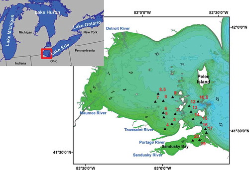
The WBLE (83–82.5 W and 41.2–41.7 N; Figure 1), with an average depth of 7 meters, is its shallowest subbasin. The WBLE is shallow enough to have dramatic wind- and wave-driven turbidity. Its relatively warm temperature makes it conducive to high biological productivity. In our study area, a number of rivers serve as conduits for fluxes of nutrients, sediment, and dissolved organic matter into the WBLE, influencing water clarity, particularly near the mouths of the Maumee, Detroit, Raisin, Sandusky, and Portage rivers (Figure 1). The WBLE is an optically complex environment due to the diversity and inhomogeneous distributions of in-water constituents (Witter et al. 2009). Resuspension of bottom sediment (Marvin et al. 2007, 2004), coupled with loading from the terrestrial environment, has resulted in a biologically productive and turbid WBLE. Variations in water quality in the WBLE are thought to be due to seasonal and interannual variability in river runoff to the lake and changes in meteorological conditions, which influence mixing, stability, and associated biological productivity (Marvin et al. 2007). In recent years, algal blooms have increased and toxic algal blooms (Microcystis and Lyngbya wollei) of the WBLE have been documented (Becker et al. 2009; Bridgeman and Penamon 2010; Rinta-Kanto et al. 2005).

Figure 1. Bathymetric map (in meter depth) of the Western Basin of Lake Erie and the locations of 18 sampling stations (in red) visited during multiple cruises on Research Vessels Gibraltar. The lake interacts with terrestrial environment through fluxes of the Sandusky, Portage, Toussaint and other rivers such as the Maumee and Detroit, which drain into the far western side of the basin. For full color versions of the figures in this paper, please see the online version.

Data acquisition

Field/lab data set

Five field cruises were conducted in the summer of 2012 during days that had relatively low cloud cover and which had an accompanying MODIS Aqua overpasses. The Ohio Stone Lab’s Research Vessel RV Gibraltar III was used for collecting samples and a suite of biogeochemical and optical measurements from 18 stations around the WBLE (Figure 1). All sampling stations were at least 2 km offshore to avoid land contamination of the collocated satellite pixels. Completion of each cruise track, which was designed to collect water samples from a variety of environments representing a wide range of optical characteristics, required approximately 11 hours. Sample locations were stored as waypoints in a marine Global Positioning System (GPS) to verify reoccupation of the same site during each cruise. For measuring chlorophyll concentrations, water samples were obtained from the near-surface mixed layer (~0.5 m). The samples were filtered through 0.45 μm glass fiber filters (GF/F) and stored in liquid nitrogen at −20°C to prevent degradation until lab analysis. Additional water samples were also collected and stored in a dark cooler for determination of TSM.

The chlorophyll a extraction process was conducted from the frozen filtered samples within 24 hours of collection following the US EPA 445 protocol (Arar and Collins 1997). Chlorophyll a pigment was extracted using 10 mL of 90% acetone buffered with MgCO₃ and macerated using a tissue grinder. The extraction process was allowed to take place for a 24-hour period in a standard refrigerator (~4°C). Chlorophyll a concentrations, which were corrected for degradation products such as pheophytin, were measured fluorometrically using a benchtop TD-700 Fluorometer (Turner Designs, Inc.) fitted with a daylight white lamp and chlorophyll optical kit (340–500 nm excitation filter and emission filter ≥ 665 nm). A three-point calibration was conducted for the optical kit using liquid chlorophyll a standards acquired from Turner design, Inc.

Satellite data

Each set of field measurements was scheduled to coincide with an overpass of the MODIS Aqua sensor. While collecting the field data at each station took up to 11 hours, the satellite images covering the entire WBLE were collected nearly instantly during the Aqua overpass at 1:30 pm local time. The field sampling campaign usually started early in the morning; therefore, data from stations that were visited in the morning will not have a perfect temporal correspondence with the data from MODIS. Due to frequent cloud cover and rainfall in the region, temporally matching data pairs are limited. Previous studies, which have considered effects of temporal variability between ground data and satellite data, have indicated that in situ data collected within ±3 days of the satellite overpass can be used for satellite matching (Bailey and Werdell 2006; Moses et al. 2009b; Witter et al. 2009). We explore the effect of temporal offsets on results in later sections.

Five MODIS Level 1A (L1A) multispectral images were selected and downloaded from the NASA Ocean Color home page (http://oceancolor.gsfc.nasa.gov/) (Table 1). The SeaWiFS Data Analysis System (SeaDAS 7) software which implements a modified atmospheric correction method (Ruddick, Ovidio, and Rijkeboer 2000) was used to convert the radiance-based values in the Level-1b data into Level-2b reflectance. The Management Unit of the North Sea Mathematical Model (MUMM) was applied to carry out atmospheric correction on the MODIS images of the WBLE. In the MUMM, the usual assumption of zero water-leaving radiance in the NIR bands is replaced by the assumption of spatial homogeneity of the 748/869 reflectance ratio for aerosol and water reflectance within an image (Ruddick, Ovidio, and Rijkeboer 2000). This ratio calculated for aerosol and water reflectance is used to determine the aerosol model. The algorithm is based on radiative transfer simulations and is designed primarily for performing atmospheric correction over turbid Case 2 waters where reflectance in the NIR is nonzero. It is adapted to a wide range of optical properties and was optimized for eutrophic European lakes that have extreme concentrations of in-water constituents. Several studies (Goyens, Jamet, and Ruddick 2013; Kahru et al. 2014; Miller and McKee 2004; Moses et al. 2009a) have successfully applied the MUMM for atmospheric correction of MODIS data in turbid waters. Compared with other NIR-based atmospheric correction procedures, the MUUM performed relatively well in the WBLE, producing positive reflectance values across the NIR spectrum, an indication that the method did not overcorrect the data (Ali, Witter, and Ortiz 2014a). During image processing, the data were mapped to a cylindrical equidistant projection with ~1 km pixel resolution, flags were raised for pixels representing coastline, land, clouds, and invalid reflectance. MODIS data from the locations of field samples delivered from cloud-free scenes and areas that were not flagged as coastline or with invalid reflectance were accepted as valid matchups. In order to retain pixel resolution and increase the signal-to-noise ratio (SNR), 3 × 3 kernel windows were used to match up with the location of sampling stations.

Table 1. Dates of each cruise and the date of the corresponding MODIS overpass of WBLE.

	Synchronous MODIS data
Field Cruise	04 June 12	11 June 12	18 June 12	26 June 12	02 July 12
MODIS overpass	06 June 12	10 June 12	19 June 12	26 June 12	04 July 12

Statistical comparison of chlorophyll a retrieval algorithms

Chlorophyll a concentrations measured from field samples were compared with spatially and temporally collocated MODIS remote sensing estimates of chlorophyll a computed from remote sensing reflectance, Rrs, using 15 bio-optical algorithms. The mathematical form of each algorithm and the numerical values of its coefficients are shown in Table 2. Standard statistical techniques were used to evaluate the satellite-based chlorophyll a concentration estimates. Least-squares regression was applied to find the best linear relationship between the field observations and the satellite-based estimates. Evaluation parameters extracted from the analyses describe the statistics of the best-fit line between the model estimates and observations (slope, intercept, and R-squared), and statistics of the model errors relative to the observations (bias, defined as the average signed deviation between the model estimate and the observations, and the root mean square error (RMSE) of the bias). These data describe the efficiency of the sensor data at detecting attenuation features associated with the chlorophyll a pigment. To evaluate whether various sources of error (CDOM, suspended sediment, the phycocyanin to chlorophyll a ratio, or atmospheric errors) may also contribute to the bias for each MODIS algorithm, we correlated the model bias, with the center-weighted derivative of the MODIS Rrs spectra. This approach allows us to see if the model errors are positively or negatively correlated with specific MODIS bands, where different sources of error have their greatest potential impact. This method of analysis is valid for comparison of errors from models even from bands that are not directly included in a model estimate because there are strong correlations between bands in the visible part of the spectrum due to electron transfer processes, which dominate the absorption features in the visible (Ortiz 2011). Simply dropping a band from a model does not necessarily exclude its potential influence from a model because spectral features can be relatively broad in the visible, resulting in the high correlation between visible bands. We then visually matched the error correlation spectra and verified the visual comparisons by calculating the correlation between each of the error correlation spectra. This allowed us to group the error correlation spectra with similar patterns to calculate an average error correlation spectrum for each grouping. In some cases, a particular algorithm exhibited a distinct spectrum that defined its own group. As final check on the quality of the groupings, we calculated the RMSE between each individual error correlation spectrum and each of the group average spectra to ensure that each individual error correlation spectrum had been assigned to the appropriate group. The average error correlation spectra can then be used to classify the algorithms on the basis of their potential source of errors as determined for this data set.

Table 2. Algorithms used to estimate chlorophyll a concentration (C) in μg/l from MODIS observations. Note that where the maximum operator (max) appears, the largest of the quantities in the square brackets is used.

Algorithm	Equations	References
		O’Reilly et al. (1998)
		O’Reilly et al. (1998)
		O’Reilly et al. (1998)
		O’Reilly et al. (1998)
		O’Reilly et al. (2000)
		O’Reilly et al. (2000)
		O’Reilly et al. (2000)
		O’Reilly et al. (2000)
		O’Reilly et al. (2000)
OC3		O’Reilly et al. (2000)
		Darecki and Stramski (2004)
		Witter et al. (2009)
		Witter et al. (2009)
NIR/red
Ali _WBLE

Results

Spatial and temporal variability of chlorophyll a

The descriptive statistics for the concentrations of chlorophyll a and TSM in the WBLE are summarized in Table 3. A total of 90 samples were collected from the various field sites during the five cruises. From these 90 samples, we obtained a subset of 47 paired-field and MODIS observations for vicarious validation of the various MODIS algorithms. Our results should be regarded as a lower limit on the joint uncertainty because few samples with very high chlorophyll a values from Sandusky Bay had valid MODIS pixels for comparison. However, this comparison constitutes a stringent test for the models since none of the data in the vicarious validation data were employed during the model development. The resulting vicarious validation statistics provide a better measure of model performance than the initial calibration statistics for each model, allowing us to test for overfitting issues related to multi-colinearity, a response to correlated input variables, or due to signal contamination arising from the interaction of multiple CPAs.

Table 3. Descriptive statistics of chlorophyll a and TSM measured during five field campaigns.

Cruise date 12	Variable	N	Mean	S.D.	Variance	Min	Max
04 June.	Chlorophyll a	18	2.67	3.68	13.52	0.42	12.07
11 June.	Chlorophyll a	18	6.96	2.37	5.62	3.71	11.65
18 June.	Chlorophyll a	18	4.15	2.65	7.01	1.21	10.41
24 June.	Chlorophyll a	18	4.84	3.91	15.29	0.88	14.94
02 July.	Chlorophyll a	18	4.85	5.74	32.98	1.15	21.19
04 June.	TSM	18	5.03	2.81	7.90	1.60	13.30
11 June.	TSM	18	2.73	4.26	18.18	0.40	16.00
18 June.	TSM	18	4.10	4.96	24.62	1.30	19.50
24 June.	TSM	18	6.39	4.43	19.64	1.90	17.80
02 July.	TSM	18	3.44	3.46	11.99	1.50	15.00

The spatial variation of chlorophyll a is depicted using data from stations that extend between Middle Bass Island in the central region of the WBLE and Sandusky Bay (Figure 2(a)). The average concentration of chlorophyll a was 2.67 µg/l in early June and 4.85 µg/l in July 2012. Relatively higher average chlorophyll a concentrations were recorded during the June 11 cruise. This can be attributed to mixing of the epilimnion with the deep chlorophyll maximum in the metalimnion as a result of stronger waves, which resulted from high winds and rainfall on that particular day (see NOAA data – https://www.ncdc.noaa.gov/cdo-web/datasets). In July, the concentrations across the basin varied between 1.15 and 21.19 µg/l, with the highest concentrations consistently recorded at stations 19 and 20, in the shallow, turbid waters of Sandusky Bay. The standard deviation of the chlorophyll a concentrations among stations showed an increasing trend from 3.68 to 5.74 µg/l between June and July. The higher standard deviation of chlorophyll a concentrations in July is attributed to the higher seasonal algal density within Sandusky Bay. During the early summer or in late spring, river discharges are high and significant amount of terrestrial matter, including nutrients, is flushed into Sandusky Bay. Riverine input makes nutrients readily available for primary producers, and this increases the productivity of the lake system. This also increases the combined concentrations of allochthonous and autochthonous phytoplankton and consequently, higher chlorophyll a concentrations are recorded at stations located nearest to or in Sandusky Bay (stations 17, 19, and 20) (Figure 1).

Figure 2. Spatial variability of (a) chlorophyll a and (b) TSM, in the WBLE during five cruise periods.

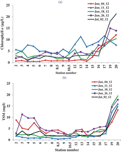
TSM concentrations in the WBLE range from 0.4 mg/l in the open waters of the central WBLE to 19.5 mg/l in the enclosed shallow Sandusky Bay. Higher than average values of TSM are recorded in early summer at the stations corresponding to Sandusky Bay relative to the stations representing the central region of WBLE, indicating difference in the optical variability between the WBLE and Sandusky Bay. Figure 2(b) shows that most of the TSM data are confined to low-level concentrations (~<5 mg/l), with only a few data points plotting at higher concentrations. This is actually influenced by the distribution of the preselected sampling stations. Most of the sampling stations are in the open waters of the WBLE where terrestrial influence is relatively low. Significantly higher TSM concentrations were recorded at stations 3, 4, 17, 19, and 20. Stations 3 and 4 are located close to the discharge zones of the Toussaint and Portage rivers and stations 17, 19, and 20 are located nearest to or in Sandusky Bay, which is a shallow basin heavily influenced by terrestrial input. This suggests that the optical properties of the waters near discharge zones are heavily influenced by terrestrially derived TSM. Ali, Witter, and Ortiz (2014b) have shown that the spatial variability of the TSM concentrations across the WBLE decreases during the summer period. This is attributed to the decreasing stream flow during the summer period coupled with the dispersion of in-water constituents into the central WBLE.

Variations in fluvial input result in large variability of chlorophyll a between the waters in Sandusky Bay and the central parts of the WBLE. Variations in nutrient dynamics in the two basins arise from differences in the dominant cyanophytes present. In Sandusky Bay, the dominant cyanophye is Planktothrix, which is nitrogen limited (Davis et al. 2015; Steffen et al. 2014) In Maumee Bay, the dominant cyanophyte is Microcystis, which is phosphorus limited (Steffen et al. 2014; Wilhelm et al. 2014). In late summer (September), river discharges decrease and as the water between the two subbasins undergoes mixing and nutrient uptake the variability of chlorophyll a in the WBLE decreases (Ali, Witter, and Ortiz 2014b; Ortiz et al. 2013; Steffen et al. 2014). The phytoplankton and cyanophyte assemblages grow in place or disperse into the open waters of WBLE and toward the Central Basin; therefore, spatial variability between the stations decreases (Ali, Witter, and Ortiz 2014b; Ortiz et al. 2013; Steffen et al. 2014; Wilhelm et al. 2014).

MODIS data

The spectral plot of the MODIS reflectance represents the net effect of the apparent optical properties of the water in the WBLE (Figure 3(a)). The reflectance values are highly variable in the visible and NIR range. The 400–800 nm spectral range displays a reflectance patterns typically observed in turbid water (Gitelson et al. 2000; Moses et al. 2009a; Schalles 2006; Wu et al. 2009), with significant absorption due to chlorophyll a and other optically active constituents, such as suspended sediment, CDOM, and important cyanophyte accessory pigments, such as phycocyanin and phycoerythrin. A local reflectance maximum, the green peak, is observed near 550 nm. This is mainly due to minimum absorption by chlorophyll a combined with scattering effects from algal cells and other suspended matter. The reflectance peak at the red/NIR edge, which is mainly due to chlorophyll a fluorescence, is apparent in the MODIS data as a weak inflection point in the reflectance derivative spectrum. The data indicate a local minimum and maximum near 667 and 678 nm: these are NIR/red attenuation features resulting from chlorophyll a absorption and emission, respectively.

Figure 3. (a) Remote sensing reflectance (Rrs) spectra of the cruise stations and (b) the derivative of the Rrs spectrum for the MODIS observations.

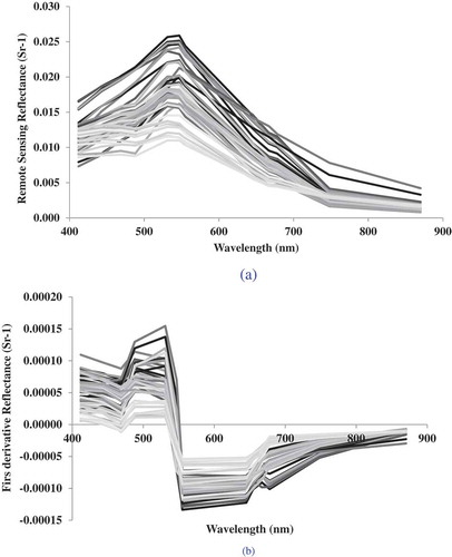
A useful way to visualize the influence of multiple CPAs on the remote sensing reflectance spectra obtained from the MODIS Aqua instrument is to calculate the derivative of the reflectance spectrum (Figure 3(b)). This removes the influence of directional effects, such as sun glint or facet reflection from waves, or differences in viewing angles, thus accentuating the diffuse reflectance arising from the interaction of the various underlying peaks and troughs among the multiple CPAs that contribute to the reflectance at each pixel (Ortiz et al. 2013). The resulting derivative spectra exhibit positive, but slightly decreasing first derivatives from 412 to 469 nm, then an increase to a broad derivative peak between 488 and 531 nm, a sharp decline toward negative derivatives at 555 nm, then a flat to gradual increase in derivatives to 645 nm, followed by variable, but generally increasing derivatives with minor peaks from 645 to 678 nm, and finally a flat or gradual increase in derivatives from 678 to 859 nm (Figure 3(b)). The derivative spectra help to minimize effects of the CDOM and suspended matter, hence emphasizing the absorption and scattering effects from phytoplankton index pigment. A thorough study has been conducted for the same lake environments by Ortiz et al. (2013), who discuss the efficiency of derivative spectra in assessing the influence of multiple associated CPAs on targeted in-water constituents, e.g., chlorophyll a.

Chlorophyll a bio-optical models

Many studies have applied the 1 models we studied to multiple sensors for the retrieval of water quality parameters in aquatic bodies (Gitelson et al. 2009; Moses et al. 2009a; O’Reilly et al. 2000; Schalles 2006; Witter et al. 2009). Regression plots between MODIS-retrieved chlorophyll a based on various algorithms and in situ chlorophyll a measurements are shown in Figure 4. Results of the statistical parameters R², slope, intercept, RMSE, and bias are listed in Table 4. In most of the selected models, MODIS data consistently overestimated the chlorophyll a concentrations at low chlorophyll a values and underestimated the chlorophyll a at high values in the WBLE, although the crossover point between the best fit and one-to-one line varies by algorithm. The global blue/green models including the Baltic and the Lake Erie regional model generated near-identical statistical parameters with an average R² of ~0.57 and RMSE ~2.9 μg/l relative to the observations. Although most of the models were normalized using the 555 nm band, their bias and RMSE varied considerably. An improved version of the Witter et al. (2009) WBLE model tuned for this data was developed using the 488/555 MODIS band ratios. The tuned model developed for this study resulted in R² = 0.62 and RMSE = 1.85 μg/l (Table 4).

Table 4. Performance and comparison of the fifteen chlorophyll a algorithms applied to MODIS data, grouped by error response and sorted by bias.

Algorithm	Statistics of the one-to-one line			Statistics relative to observations
	Slope	Intercept	R^2	Bias	RMSE
Group 1 Algorithms
Morel 2	0.59	2.65	0.59	1.19	2.13
CalCOFI two-band linear	0.50	2.57	0.59	0.78	1.94
OC3	0.52	1.48	0.58	−0.23	1.80
OC2v4	0.40	1.77	0.59	−0.38	1.89
Baltic	0.43	1.44	0.6	−0.61	1.91
Morel 1	0.30	1.93	0.46	−0.61	2.13
Morel 3	0.41	1.49	0.47	−0.62	2.04
LE Witter	0.47	0.34	0.56	−1.55	2.39
WBLE Witter	0.48	−0.18	0.55	−2.03	2.73
Ali WBLE	0.56	1.63	0.62	0.68	1.36
Group 2 Algorithm
CalCOFI three-band	0.67	2.38	0.59	1.24	2.18
Group 3 Algorithms
Morel 4	2.00	9.73	0.59	13.63	14.52
CalCOFI two-band cubic	0.58	2.17	0.58	1.47	2.42
OC4v4	0.81	1.48	0.57	0.85	2.14
Group 4 Algorithm
NIR/red	0.09	2.64	0.19	−0.64	2.45

Figure 4. Satellite chlorophyll a estimates comparisons against in situ concentration using fifteen ocean color models.

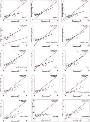
Among the blue/green models, the MODIS algorithm that produced the poorest response in the WBLE for this data set was the Morel 4 algorithm. Morel 4 overestimated all chlorophyll a values generating a slope of 2.00, intercept of 9.7, and RMSE of 14.5 μg/l relative to the observations. For all other algorithms, MODIS overestimated low chlorophyll a values, but underestimated high values of chlorophyll a, with various degrees of misfit. The OC4v4 algorithm was the one that came closest to the one-to-one line as can be seen by its slope and intercept. When the 443 nm band was used in the spectral ratio indices (Morel 1 and 3), the MODIS data generated lower correlation coefficients with respect to in situ data. This can be attributed to the greater influence of other optically active in-water constituents such as CDOM near 440 nm of the visible spectrum. This result is also apparent in the correlation of the model errors with the derivative spectra (Figure 5). Higher correlation between the measured chlorophyll a and model-based estimates was obtained for algorithms using the 490 nm band, indicating that the spectral region in the MODIS data that contains the absorption features related primarily to chlorophyll a is near 490 nm in this Case 2 environment.

Figure 5. Correlation between the derivative spectrum and model errors for the chlorophyll a algorithms grouped by response (see Table 5 for group membership list).

High positive or negative correlation between a derivative band and the model errors suggests that the CPAs that produce strong features at that particular band likely contribute to the source of error for that algorithm. Using this approach, we can group the algorithms into four classes on the basis of the correlation structure of their errors. Our approach provides insights into the underlying factors that likely contribute to the biases for each algorithm in this environment (Figure 5, Table 5; see Supplemental Appendix A).

Table 5. Distribution of algorithms by potential bias.

Source of Error	Algorithm Group 1	Algorithm Group 2	Algorithm Group 3	Algorithm Group 4
CDOM	Moderate positive	Moderate positive	Weak positive	Moderate Positive
Suspended Sediment	Moderate negative	Moderate negative	Moderate negative	Strong negative
Phycocyanin to chorlophyll a ratio	n/a	Weak negative	Weak negative	Weak positive
Atmospheric Error	Weak negative	Weak negative	Weak negative	Strong positive
Algorithms in class	Morel-2 CalCOFI two-band linear OC3 OC2v4 Baltic Morel-1 Morel-3 Witter LE Witter WBLE Ali WBLE	CalCOFI three-band	Morel-4 CalCOFI two-band cubic OC4v4	NIR/red

Various regions of the visible–NIR spectrum are influenced by multiple optically active constituents (Ortiz et al. 2013; Schalles 2006). In addition to chlorophyll a, the 400–550 nm range is influenced by CDOM and detritus which poses strong absorption coefficients, the 550–650 nm is affected by inorganics and accessory pigments, and the NIR range is more prone to scattering effects from microcystin surface scums and path radiances.

The first class of algorithms exhibits a moderate positive correlation to errors in 400–550 nm derivative bands, a moderate negative response to suspended sediment 550–650 nm, no response to bands influenced by the phycocyanin to chlorophyll a ratio, and a weak negative response to microcystin surface scum or atmospheric errors in the NIR bands. Examples of algorithms in this class include the Morel 1–3 algorithms (O’Reilly et al. 1998) and the Baltic (Darecki et al. 2003) and Regional Lake Erie algorithms (Witter et al. 2009).

The second class of algorithms exhibits a moderate positive response to CDOM-related bands, a moderate negative response to suspended sediment-related bands, a weak negative response to bands influenced by the phycocyanin to chlorophyll a ratio, and a moderate negative response to bands in the NIR influenced by microcystin surface scum or atmospheric errors. The CalCOFI three-band algorithm was the only algorithm to exhibit this response.

The third class of algorithms exhibits a very strong positive response from bands influenced by xanthophyll accessory pigments, a moderate negative response from bands influenced by suspended sediment, a weak negative response to bands influenced by the phycocyanin to chlorophyll a ratio, and a weak negative response to bands influenced by microcystin surface scum or atmospheric errors recorded in the NIR bands. The CalCOFI two-band cubic, Morel 4, and OC4v4 algorithms are in this group.

The fourth class of algorithms exhibits a weak positive response to CDOM-influenced bands, a strong negative response to bands influenced by xanthophyll accessory pigments, a weak positive response to bands influenced by the phycocyanin to chlorophyll a ratio, and a strong positive response to bands influenced by microcystin surface scum or atmospheric errors in the NIR. The red/NIR algorithms fall into this group.

Many studies (Ali, Witter, and Ortiz 2014a; Gitelson et al. 2000; Moses et al. 2009a; Ortiz et al. 2013; Schalles 2006; Witter et al. 2009) have demonstrated that in Case 2 type waters, NIR/red-based chlorophyll a models perform better than blue/green models. This is due to the fact that above 630 nm, the chlorophyll a-induced absorption signal becomes the dominant signal and accounts for nearly all absorption above 650 nm. The NIR/red bands are often less influenced by in-water constituents such as accessory pigments, CDOM, and detritus. Most notable chlorophyll a featured in this region is the in-vivo red absorption maximum of chlorophyll a near 667 nm.

In this study, chlorophyll a retrieval in the WBLE using NIR/red MODIS bands failed, generating a low slope relative to the one-to-one line, and poor R² of 0.18. The relatively low R² value may be attributed to several factors. The presence of phyocyanin, which exhibits peak absorption at 625 nm, biases the chlorophyll a signal by shifting the chlorophyll a absorption band toward the NIR, as has been shown previously using hyperspectral data from the WBLE and Sandusky Bay (Ortiz et al. 2013). This is consistent with the stronger correlation of the errors at the 667 band for the NIR/red algorithm group response. In the western basin of Lake Erie, surface scums of colonial Microcystis produce a characteristic, high spectral response in the NIR. This is the basis of the Microcystis surface scum index that is being developed by the Michigan Tech Research Institute and is currently employed to monitor the extent of the Microcystis bloom in Lake Erie. Such algorithms operate well under low wind conditions when Microcystis is able to congregate into surface mats (Hu 2009). Similar spectral responses have been observed for Sargassum, and other floating aquatic macrophytes (Hu 2009; Michalak et al. 2013).

The spectral position of the MODIS bands used in the NIR/red algorithm is also not optimal. The red absorption maximum is not well represented near the 667 nm MODIS band, and the chlorophyll a fluorescence peak (680–715 nm) is not directly detected due to the placement of a 678 nm MODIS band, which is not optimally placed in the fluorescence peak window. Likewise, the bands used in the NIR/red ratio model (678 and 753 nm) are also relatively far apart and the considerable wavelength difference over this spectral gap may lead to differences in the amount of backscattering recorded between them. The ratio procedure thus may not properly normalize for backscattering effects, which can be assumed to be similar for closely spaced wavelengths. Because the normalizing spectral band used in the NIR/red model is located at 753 nm, the measured water-leaving radiance is also extremely low resulting in a low SNR sensitive to stochastic noise or atmospheric scattering errors related to variable atmospheric path radiance. These issues reduce the efficiency of the two-band red/NIR model as applied to MODIS.

Main text paragraph

Model stability

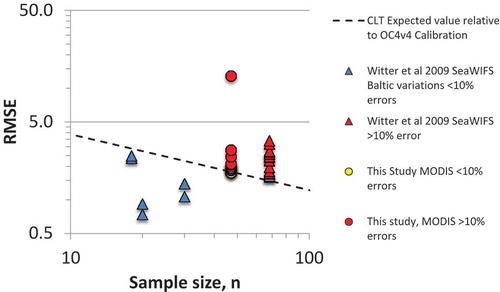
To evaluate the suitability of the various models for work in Lake Erie, we compared the results we observed with results from Witter et al. (2009) who conducted a similar exercise using SeaWIFS data and chlorophyll a observations from all three basins in Lake Erie. This allows us to test for model stability by comparing the slope, intercept, bias, and RMSE for the various models. Witter et al. (2009) had 68 sample pairs in Lake Erie, but only 18 in the WBLE. Our study increased the sample size in the WBLE to 47 data points. To normalize for differences in sample size between the two studies and to provide a global reference point, we employed the central limits theorem (CLT), and compared the Lake Erie results with the RMSE for the OC4v4 calibration data set (RMSE = 0.0231; n = 2803). This allows us to plot RMSE versus sample size for comparison against the CLT, which varies by (Figure 6). While seven of the models exhibited RMSE that was <10% of the expected value predicted by the CLT given their sample size, the remainder had errors that were larger than theoretically predicted, based on the CLT. This is not unexpected, given the fact that most of these models were initially calibrated for use in Case 1 waters. As a second test for model stability, we compared the statistics for the one-to-one line between the model estimates and observations for the two studies. The OC4v3, CalCOFI three-band, Baltic, and WBLE models from the Witter et al. (2009) study performed reasonably well in the western basin, with two or more statistics exhibiting changes of less than 25% between the two data sets. The tuned regional models from Witter et al. (2009) also produced errors that were lower than the expected value for the CLT given their sample size, indicating that the regional tuning process had reduced the observed variance relative to their calibration data set. Overall, the two studies provided comparable results.

Figure 6. The observed RMSE for the various algorithms presented as a function of samples size. The dotted line represents the expected RMSE for the OC4v4 vicarious calibration (n = 2803) extrapolated to smaller sample size based on the central limits theorem. Algorithms with RMSE values of <10% are performing as well as can be expected for the size of the vicarious calibration sample based on comparison with the central limits theorem, while those with RMSE of >10% exhibit bias that is greater than predicted by the central limits theorem.

Generally, several factors limit the potential of MODIS to accurately estimate the concentrations of chlorophyll a in turbid waters such as the WBLE. In Case 2 waters, the optical properties are also a function of non-chlorophyll a constituents such as CDOM and inorganic particles. Our results indicated that moderate-to-strong errors were contributed to most of the groups of algorithms by CDOM. Suspended sediment in this study seemed to yield moderate-to-weak negative errors as did errors associated with the interaction of phycocyanin and chlorophyll a. The lack of a strong sediment signal is not unexpected given that most of our samples were collected in regions that were not immediately adjacent to river inflow. The potential of the blue/green models is restricted due to interference from these various sources, although in this study, the greatest problems seemed to arise from CDOM. The presence of CDOM and accessory pigments likely explained the overestimation of chlorophyll a in low-chlorophyll a samples. The red edge of the spectrum is usually invoked in order to minimize the complicating influences of these accessory constituents. However, in this study, as discussed earlier, the SNR ratio in this spectral region for MODIS is low, and suboptimal band placement in the MODIS design (relative to MERIS or hyperspectral sensors) led to poorly performing NIR/red models. In addition, effects related to high reflectance in the NIR from Microcystis surface scum likely contribute to the observed errors. Optical interferences among the CPAs and the influence of path radiance due to atmospheric scattering can also be substantial, and the success of satellite remote sensing in predicting water quality parameters depends on the accuracy of the applied atmospheric correction method. For this study, the MUUM atmospheric correction model was used. This model was developed to prevent negative reflectance at shorter (400–450 nm) wavelengths. Based on visual assessment of the shape of the retrieved reflectance spectra, particularly the spectral features in the red and NIR wavelengths related to the presence of chlorophyll a, the MUUM atmospheric correction procedure implemented in the standard processing of MODIS data appears valid. The MUUM also produced NIR values that ranged from uncorrelated to only weakly correlated with the observed errors in the chlorophyll a predictions by the various algorithms. However, without synchronized in situ measurements of water-leaving radiances, it is not possible to completely assess the accuracy of the procedures from the reflectance curves alone. Implementing accurate corrections due to interference of atmospheric constituents remains a significant challenge within optical remote sensing.

Although prior studies have indicated that in situ data can be reasonably well matched within ±3 days of satellite MODIS, a sensitivity analysis was performed to evaluate the effect of temporal offsets between in situ and MODIS on vicarious calibration efforts. Variability of the physical environment may affect model performance when ground data acquisition is not well synchronized with a satellite overpass. Table 6 shows RMSE values for all models considered grouped by dates of acquisition of up to ±2 days relative to MODIS the closest temporal overpass. Results clearly show that the performance quality of the models drops with increasing temporal mismatch between the two sources of data.

Table 6. Sensitivity of models performance on the mismatches of MODIS overpass dates relative to dates of in situ observations.

	RMSE	RMSE	RMSE
Algorithm	Same day data	One day later data	Two days later data
Morel 1	0.83	2.20	2.82
Morel 2	0.96	2.11	2.95
Morel 3	0.96	2.22	2.40
CalCOFI two-band linear	0.77	1.87	2.82
CalCOFI three-band	0.87	2.23	2.93
CalCOFI two-band cubic	0.92	2.52	3.16
Morel 4	9.88	15.25	16.80
OC2v4	0.53	1.90	2.66
OC4v4	0.59	2.29	2.76
Baltic	0.84	1.96	2.60
Witter LE	1.51	2.67	2.47
Witter WBLE	1.97	3.05	2.61
OC3	0.66	1.87	2.36
NIR/red	2.07	4.43	5.07
Ali WBLE	1.18	1.18	2.54

Conclusions

Terrestrially influenced, turbid waters present serious challenges to the interpretation of diagnostic reflectance signals because of the diversity of optically active constituents, which partially masks fundamental phytoplankton absorption and scattering relationships. The chlorophyll a algorithms for Case 1 (Gordon and Morel 1983; O’Reilly et al. 1998) are universally based on a simple interaction of phytoplankton density with water. As cell densities increase, chlorophyll a-induced absorption increasingly dominates near blue wavelengths causing decreased reflectance, whereas cell scattering increasingly dominates near green (500–600 nm) wavelengths and causes increased reflectance. Hence, a simple blue to green ratio has a robust and sensitive relationship to chlorophyll a concentrations in Case 1 waters.

This simple relationship can be highly compromised in Case 2 waters where multiple optically active in-water constituents are present and therefore interfere with the chlorophyll a signal. This effect has been documented in many studies (Ali, Witter, and Ortiz 2014a, 2014b; Moses et al. 2009a; Ortiz et al. 2013) and is clearly observed in turbid waters.

Our results illustrate the potential of the MODIS satellite to estimate chlorophyll a concentrations in optically complex productive waters. The limitation of the blue/green models can primarily be attributed to the interference effects of other optically active in-water constituents such as CDOM. A second concern is the suboptimal placement of bands in the MODIS sensor relative to MERIS or hyperspectral instruments with more complete spectral coverage.

The addition of correction factors for other optically active constituents including CDOM will improve model performance, and the task of formulating the correction factors is a promising direction for future research. The comparison of the observed errors with the derivative spectrum provides a clear direction regarding how to explore model calibration and validation as suggested by our study.

To develop more robust bio-optical models, future efforts must focus on (a) improving atmospheric correction methods using physics-based approaches and enhanced calibration-validation techniques, (b) designing better field methods to accommodate for the temporal difference and effects of ground resolution between in situ and satellite data, (c) deployment of hyperspectral systems such as PACE, HyspIRI, and GEOCAPE, rather than multispectral sensors to better capture the influence of multiple CPAs, and (d) applying mathematical transformation techniques that employ the full spectral information available in the visible, rather than trying to rely on narrow-band signatures from limited band ratios. This will enhance retrievals of CPAs from satellite-based sensors and improve model stability.

Acknowledgments

We thank NASA’s South Carolina Space grant consortium and NOAA’ s Ohio Sea grant for providing funding and access. We would also like to thank Captain M. Thomas, manager of the Stone Laboratory in Putin Bay, OH, USA, for providing accommodations during the field campaign as well as piloting the RV.

Disclosure statement

No potential conflict of interest was reported by the authors.

Supplementary material

Supplemental data for this article can be accessed here.

Additional information

Funding

We thank NASA’s South Carolina Space grant consortium and NOAA’ s Ohio Sea grant for providing funding and access.

References

- Ali, K., D. Witter, and J. Ortiz. 2014a. “Application of Empirical and Semi-Analytical Algorithms to MERIS Data for Estimating Chlorophyll a in case 2 Waters of Lake Erie.” Environmental Earth Sciences 71 (9): 4209–4220. doi:10.1007/s12665-013-2814-0.
- Ali, K. A., D. L. Witter, and J. D. Ortiz. 2014b. “Multivariate Approach to Estimate Colour Producing Agents in case 2 Waters Using First-Derivative Spectrophotometer Data.” Geocarto International 29 (2): 102–127. doi:10.1080/10106049.2012.743601.
- Arar, E., and G. Collins. 1997. “In-Vitro Determination of Chlorophyll a and Pheophytin a in Marine and Freshwater Algae by Fluorescence: Cincinnati.” Ohio, National Exposure Research Laboratory, Office of Research and Development, US Environmental Protection Agency, Method EPA 445: 1–23.
- Baban, S. M. 1995. “The Use of Landsat Imagery to Map Fluvial Sediment Discharge into Coastal Waters.” Marine Geology 123 (3–4): 263–270. doi:10.1016/0025-3227(95)00003-H.
- Bailey, S. W., and P. J. Werdell. 2006. “A Multi-Sensor Approach for the On-Orbit Validation of Ocean Color Satellite Data Products.” Remote Sensing of Environment 102 (1–2): 12–23. doi:10.1016/j.rse.2006.01.015.
- Becker, R. H., M. I. Sultan, G. L. Boyer, M. R. Twiss, and E. Konopko. 2009. “Mapping Cyanobacterial Blooms in the Great Lakes Using MODIS.” Journal of Great Lakes Research 35 (3): 447–453. doi:10.1016/j.jglr.2009.05.007.
- Bridgeman, T. B., and W. A. Penamon. 2010. “Lyngbya Wollei in Western Lake Erie.” Journal of Great Lakes Research 36 (1): 167–171. doi:10.1016/j.jglr.2009.12.003.
- Bukata, R. P., J. H. Jerome, A. S. Kondratyev, and D. V. Pozdnyakov. 1995. Optical Properties and Remote Sensing of Inland and Coastal Waters. Boca Raton, FL: CRC Press.
- Casazza, G., C. Silvestri, and E. Spada. 2003. “Implementation of the Water Framework Directive for Coastal Waters in the Mediterranean Ecoregion.” Proceedings of the 6th International Conference on Mediterranean Coastal Environment (MEDCOAST 03), Ravenna, Italy, October 7–11, Vol. 2, 1157–1168.
- Cole, B. E., and J. E. Cloern. 1987. “An Empirical Model for Estimating Phytoplankton Productivity in Estuaries.” Marine Ecology Progress Series 36: 299–305. doi:10.3354/meps036299.
- Conroy, J. D., W. J. Edwards, R. A. Pontius, D. D. Kane, H. Zhang, J. F. Shea, J. N. Richey, and D. A. Culver. 2005. “Soluble Nitrogen and Phosphorus Excretion of Exotic Freshwater Mussels (Dreissena Spp.): Potential Impacts for Nutrient Remineralisation in Western Lake Erie.” Freshwater Biology 50 (7): 1146–1162. doi:10.1111/fwb.2005.50.issue-7.
- Cracknell, A., S. Newcombe, A. Black, and N. Kirby. 2001. “The ABDMAP (Algal Bloom Detection, Monitoring and Prediction) Concerted Action.” International Journal of Remote Sensing 22 (2–3): 205–247. doi:10.1080/014311601449916.
- D’Sa, E. J. 2014. “Assessment of Chlorophyll Variability along the Louisiana Coast Using Multi-Satellite Data.” GIScience & Remote Sensing 51 (2): 139–157. doi:10.1080/15481603.2014.895578.
- Dall’Olmo, G., and A. A. Gitelson. 2005. “Effect of Bio-Optical Parameter Variability on the Remote Estimation of Chlorophyll-A Concentration in Turbid Productive Waters: Experimental Results.” Applied Optics 44 (3): 412–422. doi:10.1364/AO.44.000412.
- Darecki, M., and D. Stramski. 2004. “An Evaluation of MODIS and SeaWIFS Bio-Optical Algorithms in the Baltic Sea.” Remote Sensing of Environment 89 (3): 326–350. doi:10.1016/j.rse.2003.10.012.
- Darecki, M., A. Weeks, S. Sagan, P. Kowalczuk, and S. Kaczmarek. 2003. “Optical Characteristics of Two Contrasting Case 2 Waters and Their Influence on Remote Sensing Algorithms.” Continental Shelf Research 23 (3–4): 237–250. doi:10.1016/S0278-4343(02)00222-4.
- Davis, T. W., G. S. Bullerjahn, T. Tuttle, R. M. McKay, and S. B. Watson. 2015. “Effects of Increasing Nitrogen and Phosphorus Concentrations on Phytoplankton Community Growth and Toxicity During Planktothrix Blooms in Sandusky Bay.” Lake Erie: Environmental Science & Technology 49 (12): 7197–7207.
- De Cauwer, V., K. Ruddick, Y.-J. Park, B. Nechad, and M. Kyramarios. 2004. Optical Remote Sensing in Support of Eutrophication Monitoring in the Southern. North Sea: European Association of Remote Sensing Laboratories (EARSeL).
- Dekker, A. G. 1993. Detection of Optical Water Quality Parameters for Eutrophic Waters by High Resolution Remote Sensing. Ph. D. Thesis. Proeschrift Vrije University of Amsterdam, 1–240.
- Doerffer, R., and J. Fischer. 1994. “Concentrations of Chlorophyll, Suspended Matter, and Gelbstoff in case II Waters Derived from Satellite Coastal Zone Color Scanner Data with Inverse Modeling Methods.” Journal of Geophysical Research: Oceans (1978–2012) 99 (C4): 7457–7466. doi:10.1029/93JC02523.
- El-Alem, A., K. Chokmani, I. Laurion, and S. E. El-Adlouni. 2012. “Comparative Analysis of Four Models to Estimate Chlorophyll-A Concentration in Case-2 Waters Using Moderate Resolution Imaging Spectroradiometer (MODIS) Imagery.” Remote Sensing 4 (12): 2373–2400. doi:10.3390/rs4082373.
- Gallegos, C. L., and T. E. Jordan. 2002. “Impact of the Spring 2000 Phytoplankton Bloom in Chesapeake Bay on Optical Properties and Light Penetration in the Rhode River, Maryland.” Estuaries 25 (4): 508–518. doi:10.1007/BF02804886.
- Gitelson, A. 1992. “The Peak near 700 Nm on Radiance Spectra of Algae and Water: Relationships of Its Magnitude and Position with Chlorophyll Concentration.” International Journal of Remote Sensing 13 (17): 3367–3373. doi:10.1080/01431169208904125.
- Gitelson, A., Y. Yacobi, J. Schalles, D. Rundquist, L. Han, R. Stark, and D. Etzion. 2000. “Remote Estimation of Phytoplankton Density in Productive Waters.” Advances in Limnology Stuttgart (55): 121–136.
- Gitelson, A. A., D. Gurlin, W. J. Moses, and T. Barrow. 2009. “A Bio-Optical Algorithm for the Remote Estimation of the Chlorophyll-A Concentration in case 2 Waters.” Environmental Research Letters 4 (4): 045003. doi:10.1088/1748-9326/4/4/045003.
- Gons, H. J. 1999. “Optical Teledetection of Chlorophyll a in Turbid Inland Waters.” Environmental Science & Technology 33 (7): 1127–1132. doi:10.1021/es9809657.
- Gordon, H. R., O. B. Brown, R. H. Evans, J. W. Brown, R. C. Smith, K. S. Baker, and D. K. Clark. 1988. “A Semianalytic Radiance Model of Ocean Color.” Journal of Geophysical Research: Atmospheres (1984–2012) 93 (D9): 10909–10924. doi:10.1029/JD093iD09p10909.
- Gordon, H. R., and A. Y. Morel. 1983. Remote Assessment of Ocean Color for Interpretation of Satellite Visible Imagery. New York: Springer Science & Business Media.
- Goyens, C., C. Jamet, and K. Ruddick. 2013. “Spectral Relationships for Atmospheric Correction. II. Improving Nasa’s Standard and MUMM near Infra-Red Modeling Schemes.” Optics Express 21 (18): 21176–21187. doi:10.1364/OE.21.021176.
- Gurlin, D., A. A. Gitelson, and W. J. Moses. 2011. “Remote Estimation of Chl-A Concentration in Turbid Productive Waters—Return to a Simple Two-Band NIR-Red Model?” Remote Sensing of Environment 115 (12): 3479–3490. doi:10.1016/j.rse.2011.08.011.
- Hu, C. 2009. “A Novel Ocean Color Index to Detect Floating Algae in the Global Oceans.” Remote Sensing of Environment 113 (10): 2118–2129. doi:10.1016/j.rse.2009.05.012.
- Jordan, T. E., D. L. Correll, J. Miklas, and D. E. Weller. 1991. “Long-Term Trends in Estuarine Nutrients and Chlorophyll, and Short-Term Effects of Variation in Watershed Discharge.” Marine Ecology Progress Series. Oldendorf 75 (2): 121–132. doi:10.3354/meps075121.
- Kahru, M., R. M. Kudela, C. R. Anderson, M. Manzano-Sarabia, and B. G. Mitchell. 2014. “Evaluation of Satellite Retrievals of Ocean Chlorophyll-A in the California Current.” Remote Sensing 6 (9): 8524–8540. doi:10.3390/rs6098524.
- Kahru, M., and B. G. Mitchell. 1998. “Spectral Reflectance and Absorption of a Massive Red Tide off Southern California.” Journal of Geophysical Research: Oceans (1978–2012) 103 (C10): 21601–21609. doi:10.1029/98JC01945.
- Kishino, M., T. Ishimaru, K. Furuya, T. Oishi, and K. Kawasaki. 1998. “In-Water Algorithms for ADEOS/OCTS.” Journal of Oceanography 54 (5): 431–436. doi:10.1007/BF02742445.
- Martin, S. 2004. An Introduction to Ocean Remote Sensing. New York: Cambridge University Press.
- Marvin, C., M. Charlton, J. Milne, L. Thiessen, J. Schachtschneider, G. Sardella, and E. Sverko. 2007. “Metals Associated with Suspended Sediments in Lakes Erie and Ontario, 2000–2002.” Environmental Monitoring and Assessment 130 (1–3): 149–161. doi:10.1007/s10661-006-9385-4.
- Marvin, C. H., E. Sverko, M. N. Charlton, P. A. Thiessen, and S. Painter. 2004. “Contaminants Associated with Suspended Sediments in Lakes Erie and Ontario, 1997–2000.” Journal of Great Lakes Research 30 (2): 277–286. doi:10.1016/S0380-1330(04)70345-7.
- Michalak, A. M., E. J. Anderson, D. Beletsky, S. Boland, N. S. Bosch, T. B. Bridgeman, J. D. Chaffin, et al. 2013. “Record-Setting Algal Bloom in Lake Erie Caused by Agricultural and Meteorological Trends Consistent with Expected Future Conditions.” Proceedings of the National Academy of Sciences 110 (16): 6448–6452. doi:10.1073/pnas.1216006110.
- Miller, R. L., and B. A. McKee. 2004. “Using MODIS Terra 250 M Imagery to Map Concentrations of Total Suspended Matter in Coastal Waters.” Remote Sensing of Environment 93 (1–2): 259–266. doi:10.1016/j.rse.2004.07.012.
- Mishra, D. R., B. A. Schaeffer, and D. Keith. 2014. “Performance Evaluation of Normalized Difference Chlorophyll Index in Northern Gulf of Mexico Estuaries Using the Hyperspectral Imager for the Coastal Ocean.” GIScience & Remote Sensing 51 (2): 175–198. doi:10.1080/15481603.2014.895581.
- Morel, A., and L. Prieur. 1977. “Analysis of Variations in Ocean Color1.” Limnology and Oceanography 22 (4): 709–722. doi:10.4319/lo.1977.22.4.0709.
- Morrow, J. H., B. N. White, M. Chimiente, and S. Hubler. 2000. “A Bio-Optical Approach to Reservoir Monitoring in Los Angeles, California.” Advances in Limnology 55: 179–191. Stuttgart.
- Moses, W. J., A. A. Gitelson, S. Berdnikov, and V. Povazhnyy. 2009a. “Estimation of Chlorophyll-A Concentration in case II Waters Using MODIS and MERIS Data—Successes and Challenges.” Environmental Research Letters 4 (4): 045005. doi:10.1088/1748-9326/4/4/045005.
- Moses, W. J., A. A. Gitelson, S. Berdnikov, and V. Povazhnyy. 2009b. “Satellite Estimation of Chlorophyll-Concentration Using the Red and NIR Bands of MERIS—The Azov Sea Case Study.” Geoscience and Remote Sensing Letters, IEEE 6 (4): 845–849. doi:10.1109/LGRS.2009.2026657.
- Nellis, M. D., J. A. Harrington, and J. Wu. 1998. “Remote Sensing of Temporal and Spatial Variations in Pool Size, Suspended Sediment, Turbidity, and Secchi Depth in Tuttle Creek Reservoir, Kansas: 1993.” Geomorphology 21 (3–4): 281–293. doi:10.1016/S0169-555X(97)00067-6.
- O’Reilly, J. E., S. Maritorena, D. A. Siegel, M. C. O’Brien, D. Toole, B. G. Mitchell, M. Kahru, F. P. Chavez, P. Strutton, and G. F. Cota. 2000. Ocean Color Chlorophyll a Algorithms for SeaWIFS, OC2, and OC4: Version 4: SeaWIFS Postlaunch Calibration and Validation Analyses, Part, Vol. 3, 9–23. Washinton, DC: American Geophysical Union.
- O’Reilly, J. E., S. Maritorena, B. G. Mitchell, D. A. Siegel, K. L. Carder, S. A. Garver, M. Kahru, and C. McClain. 1998. “Ocean Color Chlorophyll Algorithms for SeaWIFS.” Journal of Geophysical Research: Oceans (1978–2012) 103 (C11): 24937–24953. doi:10.1029/98JC02160.
- Ortiz, J. D. 2011. “Application of Visible/Near Infrared Derivative Spectroscopy to Arctic Paleoceanography.” IOP Conference Series Earth and Environmental Science 14(1). doi:10.1088/1755-1315/14/1/012011.
- Ortiz, J. D., D. L. Witter, K. A. Ali, N. Fela, M. Duff, and L. Mills. 2013. “Evaluating Multiple Colour-Producing Agents in case II Waters from Lake Erie.” International Journal of Remote Sensing 34 (24): 8854–8880. doi:10.1080/01431161.2013.853892.
- Ouillon, S., P. Douillet, and S. Andréfouët. 2004. “Coupling Satellite Data with in Situ Measurements and Numerical Modeling to Study Fine Suspended-Sediment Transport: A Study for the Lagoon of New Caledonia.” Coral Reefs 23 (1): 109–122. doi:10.1007/s00338-003-0352-z.
- Pettersson, L., D. Durand, O. Johannessen, E. Svendsen, T. Noji, H. Soeiland, and P. Regner. 2000. “Satellite Observations and Model Predictions of Toxic Algae Blooms in Coastal Waters.” Proceedings the Fifth Pacific Ocean Remote Sensing Conference (PORSEC), Goa, India, December 4–8, 2000, Vol. 1, 657–661.
- Pozdnyakov, D., R. Shuchman, A. Korosov, and C. Hatt. 2005. “Operational Algorithm for the Retrieval of Water Quality in the Great Lakes.” Remote Sensing of Environment 97 (3): 352–370. doi:10.1016/j.rse.2005.04.018.
- Rinta-Kanto, J., A. Ouellette, G. Boyer, M. Twiss, T. Bridgeman, and S. Wilhelm. 2005. “Quantification of Toxic Microcystis Spp. during the 2003 and 2004 Blooms in Western Lake Erie Using Quantitative Real-Time PCR.” Environmental Science & Technology 39 (11): 4198–4205. doi:10.1021/es048249u.
- Rowan, K. S. 1989. Photosynthetic Pigments of Algae. New York: Cambridge University Press.
- Ruddick, K. G., F. Ovidio, and M. Rijkeboer. 2000. “Atmospheric Correction of SeaWIFS Imagery for Turbid Coastal and Inland Waters.” Applied Optics 39 (6): 897–912. doi:10.1364/AO.39.000897.
- Schalles, J. F. 2006. “Optical Remote Sensing Techniques to Estimate Phytoplankton Chlorophyll a Concentrations in Coastal.” Remote Sensing of Aquatic Coastal Ecosystem Processes 9: 27–79.
- Schmugge, T. J., W. P. Kustas, J. C. Ritchie, T. J. Jackson, and A. Rango. 2002. “Remote Sensing in Hydrology.” Advances in Water Resources 25 (8–12): 1367–1385. doi:10.1016/S0309-1708(02)00065-9.
- Shuchman, R., A. Korosov, C. Hatt, D. Pozdnyakov, J. Means, and G. Meadows. 2006. “Verification and Application of A Bio-Optical Algorithm for Lake Michigan Using SeaWIFS: A 7-Year Inter-Annual Analysis.” Journal of Great Lakes Research 32 (2): 258–279. doi:10.3394/0380-1330(2006)32[258:VAAOAB]2.0.CO;2.
- Simis, S. G., S. W. Peters, and H. J. Gons. 2005. “Remote Sensing of the Cyanobacterial Pigment Phycocyanin in Turbid Inland Water.” Limnology and Oceanography 50 (1): 237–245. doi:10.4319/lo.2005.50.1.0237.
- Steffen, M. M., Z. Zhu, R. M. L. McKay, S. W. Wilhelm, and G. S. Bullerjahn. 2014. “Taxonomic Assessment of a Toxic Cyanobacteria Shift in Hypereutrophic Grand Lake St. Marys (Ohio, USA).” Harmful Algae 33: 12–18. doi:10.1016/j.hal.2013.12.008.
- Tarrant, P., and S. Neuer. 2009. “Monitoring Algal Blooms in a Southwestern US Reservoir System.” Eos, Transactions American Geophysical Union 90 (5): 38–39. doi:10.1029/2009EO050002.
- Torbick, N., F. Hu, J. Zhang, J. Qi, H. Zhang, and B. Becker. 2008. “Mapping Chlorophyll-A Concentrations in West Lake, China Using Landsat 7 ETM+.” Journal of Great Lakes Research 34 (3): 559–565. doi:10.3394/0380-1330(2008)34[559:MCCIWL]2.0.CO;2.
- Wilhelm, S. W., G. R. LeCleir, G. S. Bullerjahn, R. M. McKay, M. A. Saxton, M. R. Twiss, and R. A. Bourbonniere. 2014. “Seasonal Changes in Microbial Community Structure and Activity Imply Winter Production Is Linked to Summer Hypoxia in a Large Lake.” FEMS Microbiology Ecology 87 (2): 475–485. doi:10.1111/1574-6941.12238.
- Witter, D. L., J. D. Ortiz, S. Palm, R. T. Heath, and J. W. Budd. 2009. “Assessing the Application of SeaWIFS Ocean Color Algorithms to Lake Erie.” Journal of Great Lakes Research 35 (3): 361–370. doi:10.1016/j.jglr.2009.03.002.
- Wu, M., W. Zhang, X. Wang, and D. Luo. 2009. “Application of MODIS Satellite Data in Monitoring Water Quality Parameters of Chaohu Lake in China.” Environmental Monitoring and Assessment 148 (1–4): 255–264. doi:10.1007/s10661-008-0156-2.
- Yentsch, C. S. 1960. “The Influence of Phytoplankton Pigments on the Colour of Sea Water.” Deep Sea Research (1953) 7 (1): 1–9. doi:10.1016/0146-6313(60)90002-2.