Integration of full-waveform LiDAR and hyperspectral data to enhance tea and areca classification

Abstract

Hyperspectral image and full-waveform light detection and ranging (LiDAR) data provide useful spectral and geometric information for classifying land cover. Hyperspectral images contain a large number of bands, thus providing land-cover discrimination. Waveform LiDAR systems record the entire time-varying intensity of a return signal and supply detailed information on geometric distribution of land cover. This study developed an efficient multi-sensor data fusion approach that integrates hyperspectral data and full-waveform LiDAR information on the basis of minimum noise fraction and principal component analysis. Then, support vector machine was used to classify land cover in mountainous areas. Results showed that using multi-sensor fused data achieved better accuracy than using a hyperspectral image alone, with overall accuracy increasing from 83% to 91% using population error matrices, for the test site. The classification accuracies of forest and tea farms exhibited significant improvement when fused data were used. For example, classification results were more complete and compact in tea farms based on fused data. Fused data considered spectral and geometric land-cover information, and increased the discriminability of vegetation classes that provided similar spectral signatures.

Keywords:

• land-cover classification
• waveform LiDAR
• hyperspectral image
• data fusion
• principal component analysis
• minimum noise fraction

1. Introduction

Hyperspectral remote sensing is an effective optical technique for acquiring land-use and land-cover data to increase understanding of the earth’s surface (Zhang and Zhu 2011). The basic concept of optical imaging is that the amount of radiation that is reflected, absorbed, or emitted by any material varies with wavelength. Hyperspectral imaging sensors provide radiance information of materials at a large number of spectral wavelength bands (Manolakis, Marden, and Shaw 2003), thus resulting in detailed spectral information of the material. These data are useful in determining land-cover mapping and in delineating the extent of land-cover classes (Petropoulos, Arvanitis, and Sigrimis 2012). Recently, the emerging technique of airborne light detection and ranging (LiDAR) has provided accurate vertical structure information that acquires 3D geometric information of land-use and land-cover features (Sun and Salvaggio 2012; Akay et al. 2009; Chu et al. 2014). Such techniques can be useful in describing forest geometric parameters, such as canopy height and stand volume (Nilsson 1996; Bolton, Coops, and Wulder 2013). LiDAR systems also have potential in classifying land cover. Information from airborne LiDAR data, such as elevation and intensity, is used to classify land-cover types efficiently (Zhang, Xie, and Selch 2013). Moreover, airborne LiDAR systems record the entire point frequency distributions and provide sufficient information on the geometric distribution of surfaces to classify land cover (Antonarakis, Richards, and Brasington 2008). Given their different characteristics (Hall et al. 2009), hyperspectral imaging and LiDAR sensors can provide spectral and geometric information on land cover with accurate classification. Dalponte, Bruzzone, and Gianelle (2008) classified forest areas in fusing LiDAR and hyperspectral data. Elevation and intensity information in LiDAR data, which were converted into a raster image, were incorporated into hyperspectral image data. Onojeghuo and Blackburn (2011) acquired airborne hyperspectral and LiDAR imagery from two sites in Cumbria, United Kingdom. LiDAR-derived measures can generate a digital surface model (DSM), DSM-derived slope maps, and a canopy height model. They combined this LiDAR height information into the principal components of imagery features to classify land cover.

Data fusion is usually applied for the integration of multi-sensor data to improve the performance of land-cover mapping and to enhance visual interpretation (Lu et al. 2011). Dalponte, Bruzzone, and Gianelle (2012) integrated multi-sensor data sets, including airborne hyperspectral images and LiDAR information (i.e., tree height) to classify land cover. Results showed that integrating these data was useful in identifying tree species. However, hyperspectral images cover a large number of bands, whereas full-waveform LiDAR data collect a high-frequency sampling signal for each pulse. The large number of dimensions from both data sources results in high computational complexity. Reducing data dimensionality is essential to prevent inferior discrimination when making classifications from large data. Principal component analysis (PCA) and maximum noise fraction (MNF) are introduced as data dimensionality reduction algorithms in remote-sensing image classification (Xia et al. 2014). After reducing data dimensionality, the overall accuracy of land-cover classification generally improved compared with using all original data. MNF and PCA were used to integrate various data sets into a new data set by using multi-sensor features. Mutlu et al. (2008) applied such dimension reduction approaches, including MNF or PCA, to extract the main features of LiDAR and multispectral data for land-cover classification. Results from previous studies (Mutlu et al. 2008; Guo et al. 2011) have shown that classifying land cover exhibited better performance in combination of LiDAR and multispectral data compared with using multispectral data alone. Wang, Tseng, and Chu (2014) extracted waveform information of LiDAR data for land-cover classification. However, preprocessing waveform LiDAR data includes waveform decomposition (Wagner et al. 2006), ground point extraction, and choosing the appropriate LiDAR-derived indices (e.g., the mean, standard deviation, or maximum/minimum value of LiDAR points within a unit area; Antonarakis, Richards, and Brasington 2008). In the current study, we proposed a data fusion method that can be applied directly to supervised classification without the abovementioned preprocessing. Multi-sensor data, such as hyperspectral data and waveform LiDAR information, can be extracted effectively by MNF and PCA.

The objectives of this study are as follows: (1) to develop an effective multi-sensor data fusion method that employs hyperspectral and full-waveform LiDAR data for classifying land cover, and (2) to demonstrate the usefulness of fused data in classifying land cover. Airborne hyperspectral images and waveform LiDAR data can generate high spatial and spectral resolution data. Data fusion approaches, that is, MNF and PCA, that integrate hyperspectral and LiDAR data were used to improve the overall accuracy of classifying land cover. Furthermore, the results of land-cover classification derived from using hyperspectral data alone and from using fused data (i.e., combined dimensionally reduced hyperspectral and full-waveform LiDAR data) were compared to demonstrate the benefits of fusing the two types of data to classify land cover. Fusing multi-sensor data can improve the overall accuracy of classifying land cover, particularly in vegetation regions.

2. Study area and material

The Tseng-Wen Reservoir is the largest multipurpose reservoir in Taiwan. The mountainous watershed is located in the upstream area of the Tseng-Wen River system in Chiayi County. The entire area of the river basin is 1176 km², of which the mountainous watershed covers 481 km². Our study area is located in the upstream of the mountainous watershed and measures 5000 × 7000 m². The average elevation and slope are approximately 610 m and 24°, respectively.

Airborne hyperspectral data were acquired using the CASI-1500 hyperspectral imager (ITRES, Alberta, Canada). This sensor provided reflectance data with measured 72 bands that cover the visible and near-infrared regions of the spectrum from 362.8 nm to 1051.3 nm, with a spectral resolution of 9.6 nm. Hyperspectral imagery with 1 m ground sample distance (GSD) was collected over the study area on 13 September 2012 through an aircraft at a height of 1800 m with a field of view (FOV) of 40°. A total of nine strips were acquired. The empirical line method (Mutlu et al. 2008), where cement and asphalt surfaces were used as the bright and dark surfaces, respectively, was used for the atmospheric correction procedure. All surfaces were measured by a PSR-1100 field portable spectroradiometer (Spectral Evolution, USA). Given the poor correction results within the spectral range of 362.8 nm to 391.6 nm and 902.8 nm to 979.4 nm, the 12 bands were discarded.

Waveform LiDAR data sets were collected on 2 September 2012 (most land cover remained unchanged between the surveys.). Airborne LiDAR data were acquired using an Optech ALTM Pegasus LiDAR system (Optech Incorporated, Ontario, Canada) at the altitude of 1800 m. The laser source emits pulses at the wavelength of 1064 nm with a pulse rate of 100 KHz, scan rate of 22 Hz, and FOV of 24°. The strip side overlap was more than 50%, and the density from the first return was approximately 2.4 point/m² in the study area. Aerial photographs were collected simultaneously during the surveys. Orthorectification of the hyperspectral data was conducted based on the DSM obtained from the LiDAR data. GPS and inertial measurement unit were used to acquire the position and orientation information. The horizontal position accuracies of the hyperspectral and LiDAR data were estimated to be 2 and 0.3 m, respectively.

3. Method

3.1 Overall and data processing

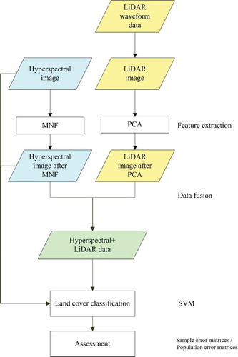
Figure 1 illustrates the data fusion procedure for LiDAR and hyperspectral data in land-cover classification. First, the LiDAR image with 256 height-bin layers was generated from full-waveform LiDAR data. The intensity of full-waveform LiDAR data was discretized with 256 height bins, separated by 1 ns. Although LiDAR data were collected at a point density of 2.4 points/m², the LiDAR point clouds were distributed unevenly. The waveform LiDAR data were rasterized by averaging all the waveforms in each grid. The waveforms were assigned based on the positions of the last return for multiple-return waveforms. To ensure at least one LiDAR waveform for each grid, LiDAR data were rasterized at a 2 m grid size. Moreover, a 2 m GSD hyperspectral image was aggregated to match the spatial resolution of the LiDAR image. Next, fusing LiDAR and hyperspectral data based on MNF and PCA was considered. After extracting the major components of hyperspectral and LiDAR data, supervised classification was applied to classify land cover based on the fused data set. Details of feature extraction, data fusion, and classification are shown as follows.

Figure 1. Flowchart of the proposed method for multi-sensor feature extraction, data fusion, land-cover classification, and accuracy assessment.

3.2 Feature extraction and data fusion

This study applied PCA and MNF to extract major features of multi-sensor data for classifying land cover. PCA is a dimension reduction technique that acquires a low-dimensional linear representation of data vectors to reconstruct the original data from the compressed information (Ilin and Raiko 2010). This technique converts a set of possibly correlated waveform LiDAR data into principal components that are uncorrelated variables. The major principal components are extracted from high-dimensional LiDAR data. Meanwhile, MNF determines the dimensionality of hyperspectral image data, separates noise from the data, and reduces computational time for processing (Boardman and Kruse 1994). An MNF transform primarily includes two coupled principal component transformations (Green et al. 1988). The first transformation, which is applied to an estimated noise covariance matrix, decorrelates any noise in the data. The second one is the principal component transformation that creates new bands with the majority of information. The inherent dimensionality of the hyperspectral data can be determined by examining the eigenvalues, thus allowing further classification processing. The PCA and MNF for the LiDAR image and hyperspectral data were both conducted in ENVI 5.0 (Exelis Visual Information Solutions, Colorado, USA). With the use of MNF, a homogeneous area for calculating noise statistics should be defined first. In this study, an asphalt road surface was used to estimate noise information of the hyperspectral data. Defining the homogeneous area directly from LiDAR data is difficult. Thus, MNF was applied for hyperspectral data, while PCA was used for LiDAR data.

In data fusion, this study preserved the major components, including 13 MNFs in the hyperspectral images and 7 PCAs in LiDAR data, each of which contributed more than 1% of variance in the transformed data.

3.3 Land-cover classification and accuracy assessment

To prove the classification performance from multi-sensors, support vector machine (SVM) was used to estimate land-cover classes. SVM is one of the most discriminative supervised classification approaches in remote sensing (Melgani and Bruzzone 2004; Mountrakis, Im, and Ogole 2011; Tseng et al. 2015). It is the superior machine learning algorithm in classifying high-dimensional data sets (Huang, Davis, and Townshend 2002). It can consider the associated statistical theory to determine the optimal separation of classes and effectively separate nonlinearly separable data in a high-dimensional space induced by the kernel function (Vapnik 2000). In this study, the radial basis function kernel was chosen to produce good results. The formulation of the SVM classifier can be referred to Chang and Lin (2011). The SVM classifier is implemented by using the functions from ENVI 5.0. The major parameters of SVM include the gamma in the kernel function and the penalty parameter. The gamma was set to a value equal to the inverse of the number of spectral bands of the imagery, whereas penalty parameter was set as 1600 to determine the trade-off between the training error and complexity of the model.

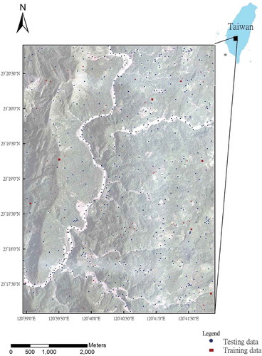
In the study area, land-cover types were mainly classified into forest, built-up, low vegetation (grass), water, tea farm, betel palm (areca) farm, and bare land. Clouds and shadows were excluded by using masks in the accuracy assessment. Reflectance signatures of land-cover classes in the hyperspectral image are shown in Figure 2. Reflectance signatures in forests are similar to those of tea and areca. However, distinctions among vegetation types are often identified from leaf size and shape, water content, plant shape, and associated background. Figure 3 shows the locations of the training and testing data. The SVM outperforms other methods using limited training samples (Shao and Lunetta 2012). Less than 1% of the total data were selected as training data in the classifier. The samples must be clearly recognizable and nearly pure. Independent samples were randomly selected as test data. Reflectance signatures of the hyperspectral image and aerial photographs with 0.25 m GSD were used as references. After the points were manually checked, 512 pixels were used as ground reference data for accuracy validation (assessment). The overall user and producer accuracies from the sample error matrix and population error matrices were used in accuracy assessment (Stehman and Foody 2009). Overall accuracy denotes the total classification accuracy (i.e., the ratio of the number of correctly classified pixels to the total number of validation pixels used in all classes). User accuracy indicates the probability that a classified data sample represents the ground reference category, whereas producer accuracy denotes the probability that all surveyed ground reference points are classified under the same land-cover class by the map producer. Moreover, sample ratio corrections in weighting the samples by the area of the land-cover type can be applied in the population error matrix (Stehman and Foody 2009).

Figure 2. Reflectance signatures of (a) areca, (b) forest, (c) tea, (d) grass, (e) bare, (f) built-up area, and (g) water in the hyperspectral images (thick line: average of reflectance signatures; brown area: range of reflectance signatures). For full color versions of the figures in this paper, please see the online version.

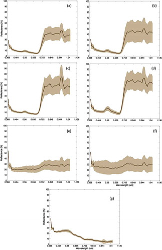
Figure 3. Locations of training and testing data in land-cover classification.

4. Results and discussion

4.1 Data fusion via MNF and PCA

Figure 4 shows the total variance among feature dimensions explained by the leading MNF and PCA. This study preserved the major components (i.e., more than 1% of the total variance), including 13 MNFs in the hyperspectral images (60 bands) and 7 PCAs in LiDAR data (255 height-bins). Independent major features can be extracted based on hyperspectral and LiDAR data after MNF and PCA. The multi-sensor fused data (HYPER + LiDAR) contain 13 major features of hyperspectral imagery extracted by MNF and 7 PCAs extracted from LiDAR data. The first five PCAs of LiDAR data are shown in Figure 5. Compared with LiDAR-derived digital elevation model (DEM) (Figure 6), the PCA data imply terrain elevation and geometric information of land cover. For example, PCA1 shows the terrain surface in which the bright color represents the river and the dark color represents the mountainous area in the study area (i.e., correlation coefficient is −0.6 between the PCA1 and DEM). Thus, PCAs and MNFs can provide complementary information (e.g., vertical structure in LiDAR data and spectral reflectance in a hyperspectral image). The major principal components (either from MNF or PCA) typically capture the largest amount of information, thereby guaranteeing minimal information loss of reconstruction (Guan and Dy 2009). MNF and PCA transform the original data with large dimensionality into data with reduced dimensionality and maintain as much information content as possible. Dimension reduction is important in high-dimensional classification problems. In the present study, some major principal components contain significant discontinuity along the perimeters of the flight line stripes. Thus, the components were discarded and excluded from further analysis.

Figure 4. Total variance of feature dimensions explained by leading dimensions.

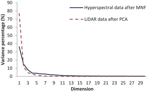
Figure 5. First five PCAs from LiDAR data.

Figure 6. LiDAR-derived DEM.

4.2 Classification accuracy of fused data

Figure 7 shows the classification results based on hyperspectral data alone (HYPER, Figure 7b), hyperspectral data after MNF (HYPER_MNF, Figure 7c), and hyperspectral and LiDAR fused data (HYPER + LiDAR, Figure 7d). The classification overall accuracy results using SVM and maximum likelihood estimation (MLE) are shown in Table 1. Overall accuracies from sample error matrices for HYPER, HYPER_MNF, and HYPER + LiDAR are 87%, 88%, and 90% using SVM, respectively. Values in overall accuracies for HYPER, HYPER_MNF, and HYPER + LiDAR using MLE are 85%, 86%, and 89% from sample error matrices, respectively. Using MLE, overall accuracies are 78%, 81%, and 87% for HYPER, HYPER_MNF, and HYPER + LiDAR from population error matrices, whereas overall accuracies are 83%, 85%, and 91% using SVM for HYPER, HYPER_MNF, and HYPER + LiDAR from population error matrices, respectively. HYPER + LiDAR exhibits the highest overall accuracy, followed by HYPER_MNF, whereas HYPER has the lowest values. Various data sets exhibit consistent classification results, that is, major land-cover classes can be identified effectively using SVM. The error matrices of classifications using SVM based on HYPER, HYPER_MNF, and HYPER + LiDAR are shown in the Appendix. However, several tea and areca farms are misclassified as forests, and some built-up areas are misclassified as bare land.

Table 1. Overall accuracy of SVM and MLE using hyperspectral data alone (HYPER), hyperspectral data after MNF (HYPER_MNF), and multi-sensor data (HYPER + LiDAR) from sample and population error matrices.

	Sample overall accuracy		Population overall accuracy
	SVM	MLE	SVM	MLE
HYPER	0.87	0.85	0.83	0.78
HYPERMNF	0.88	0.86	0.85	0.81
HYPER + LiDAR	0.90	0.89	0.91	0.87

Figure 7. (a) Hyperspectral image (R: 654.9 nm; G: 559.4 nm; B: 454.1 nm), and land-cover classification using (b) hyperspectral data alone (HYPER), (c) hyperspectral data after MNF (HYPER_MNF), and (d) multi-sensor data (HYPER + LiDAR) based on SVM.

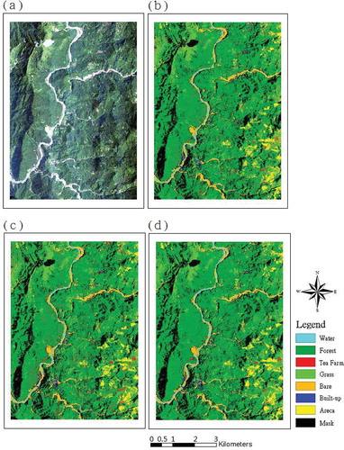
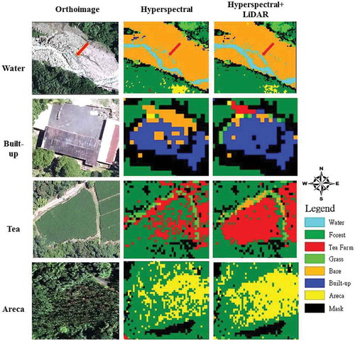
Figure 8 shows the SVM result comparisons using HYPER and multi-sensor (HYPER + LiDAR) data in water, built-up, tea, and areca. Using fused data, the classification errors, in which areca and tea are misclassified as forest, can be improved (Figure 8). Furthermore, the patterns of water, bare, tea farm, and areca farm are continuous but not fragmented when using fused data. In various land-cover types, the classification results based on fused data are more complete/compact than those based on hyperspectral data (Figure 8). Salt-and-pepper noise (high local variation) from a pixel-based classification can be reduced by the data fusion. Thus, the classification result based on fused data is more reasonable and feasible for classifying land cover than the result based on hyperspectral image only. To overcome the salt-and-pepper effect from the classification, the fused data will be suggested for land-cover classification.

Figure 8. SVM result comparisons using HYPER and HYPER + LiDAR data in water, built-up, tea, and areca (pixel sizes were 2 m in classification images and 0.25 m in orthoimage).

Table 2 shows the comparison between user accuracy and producer accuracy of SVM classifications from population error matrices. User accuracy is improved by 2.4% in forests when HYPER_MNF was used compared with HYPER. It also improved by approximately 8% in forests by using HYPER + LiDAR compared with HYPER. Meanwhile, producer accuracy is improved by 4% in tea farm, 2% in areca farm, and 1% in grass when HYPER + LiDAR was used compared with HYPER. In summary, the classification accuracies of forest, tea farm, and areca farm exhibit significant improvements in classifying land cover by using HYPER + LiDAR compared with HYPER. The result particularly proves this point by using the fused data, where in the areca and tea farms are misclassified as forests based on the population error matrices.

Table 2. Producer accuracy and user accuracy in various data sources using HYPER, HYPER_MNF, and HYPER + LiDAR from population error matrices based on SVM.

	Producer accuracy (%)			User accuracy (%)
	HYPER	HYPERMNF	HYPER + LiDAR	HYPER	HYPERMNF	HYPER + LiDAR
Areca	94.6	94.7	97.4	99.7	99.8	99.7
Forest	99.7	99.6	99.7	85.4	87.8	93.2
Tea	95.3	96.8	99.1	100.0	99.9	100.0
Grass	95.3	96.0	96.4	99.7	99.7	99.8
Bare	99.9	99.9	99.9	98.1	97.8	98.2
Built-up	98.2	98.0	98.3	100.0	100.0	100.0
Water	99.9	99.9	100.0	100.0	100.0	100.0

Most multi-sensor data classification methods have common problems, such as high dimensionality of feature spaces and feature selection (Ari and Aksoy 2010). Generally, physical-based features from airborne LiDAR data, such as height, slope indices, and waveform features, are used to classify land-cover types efficiently (Dalponte, Bruzzone, and Gianelle 2012; Wang, Tseng, and Chu 2014). However, the physical-based features were difficult to extract from the LiDAR data; for example, forest canopy is not solely a function of tree height but also a function of canopy closure (Lim et al. 2003). Tree height estimation from LiDAR data is case by case in the heterogeneous environment, for example, tree height estimation accuracy varies on flat and sloped terrains (Drake et al. 2002; Lefsky et al. 2007). The process of extracting physical-based features using waveform LiDAR data is usually detailed. In the study, effective waveform LiDAR information can be extracted directly by PCA. Data preprocessing, such as waveform decomposition or ground point extraction, can be ignored in our approach. The major features of hyperspectral imagery and waveform LiDAR data extracted by MNF and PCA still achieve the accuracy required for classifying land cover. However, for vegetation classes, only hyperspectral data do not exhibit excellent accuracy. The task of separating forest, tea farm, and areca farm is challenging if only hyperspectral data are used. Fused data are effective in distinguishing forest, tea farm, and areca farm because LiDAR data can provide unique information about them (e.g., height and intensity) (Heinzel and Koch 2011; Sasaki et al. 2012). Our results prove previous studies (Heinzel and Koch 2011), in which waveform LiDAR data have the most critical role in increasing discriminability and accuracy of vegetation species classes if land cover exhibits similar spectral signatures. The fused data considering both spectral and geometric land-cover information increase vegetation class discriminability. In addition, Table 3 shows that the sensitive analysis of areca, tea, and overall accuracy in the classification if a feature is excluded. Overall accuracy is not sensitive to the features from 88% to 90%, but areca accuracy is sensitive from 85% to 96%. The MNF9, MNF5, and PCA1 are most critical features in areca classification. Moreover, tea accuracy is not highly sensitive except excluding MNF6. The critical features in tea classification are MNF6, MNF1, PCA2, PCA3, and MNF8. The result implies that most PCA and MNF features are critical and reliable in the classification, but their effects are various in areca and tea.

Table 3. Sensitive analysis of classification for areca, tea and overall accuracy from samples (Unit: %).

Excluding feature	Areca accuracy	Tea accuracy	Overall accuracy
No excluding	94.2	96.7	90.4
PCA6	96.2	100.0	90.0
MNF3	96.2	100.0	88.3
MNF8	94.2	93.3	90.6
PCA7	94.2	100.0	89.6
MNF4	94.2	96.7	89.6
MNF2	94.2	100.0	89.3
MNF11	92.3	96.7	90.4
MNF10	92.3	100.0	90.0
MNF12	92.3	96.7	89.6
PCA5	92.3	96.7	89.5
PCA4	92.3	100.0	89.3
MNF13	90.4	100.0	89.8
MNF7	90.4	96.7	89.6
PCA2	90.4	93.3	89.3
MNF1	90.4	90.0	88.7
MNF6	90.4	76.7	88.7
PCA3	90.4	93.3	87.9
PCA1	88.5	100.0	89.6
MNF5	88.5	100.0	89.1
MNF9	84.6	96.7	89.3

Combinations of hyperspectral/multispectral image and LiDAR data are increasingly being used to map land cover (Ke, Quackenbush, and Im 2010; Alexander et al. 2010; Guo et al. 2011). Our data fusion for classifiers is effective when these data sources, such as hyperspectral data (60 bands) and full-waveform LiDAR information (255 height-bins), are considered. Hyperspectral images can obtain an entire spectrum for each grid, whereas full-waveform LiDAR data can acquire vertical information and explore land cover with geometric structures. Waveform LiDAR systems record the entire return signal from all illuminated surfaces (Lefsky et al. 2007). Previous studies considered only canopy height or ground elevation information of LiDAR data when fusing image data (Dalponte, Bruzzone, and Gianelle 2008). However, extracting canopy height or ground elevation information from waveform LiDAR data requires confirmation. Inaccurate canopy height will be extracted from LiDAR data if canopy closure and density influence laser response significantly (Lim et al. 2003). Inaccurate canopy height results in poor land-cover classification. In our approach, canopy height or ground elevation information is not required but is possibly hidden in the PCAs. On the basis of the results, the fusion of the effective independent information in multi-sensor data is significant in reducing salt-and-pepper noise from classifying land cover.

5. Conclusion

Hyperspectral images contain a large number of bands to provide land-cover discrimination with various reflectances at all wavelengths. By contrast, waveform LiDAR systems record the entire time-varying intensity of a return signal for detailed geometric information of land cover. This study used data fusion approaches (MNF and PCA) to integrate multi-sensor data and then applied SVM to delineate major land-cover patches based on the fused data. Results indicate that the methods are suitable for fusing high-dimensional hyperspectral and waveform LiDAR data. Dominant features can be determined using data fusion approaches for land-cover classification.

Various data sets exhibit generally consistent classification results, that is, major land-cover types can be identified effectively using SVM. However, results show that HYPER + LiDAR provides the most accurate land-cover clusters. Fused data (7 PCAs and 13 MNFs) offer several benefits, including extensions that consider the geometric and spectral information of land cover. Fused data demonstrated better accuracy than using HYPER, with overall accuracy increasing from 83% to 91% using population error matrices. To reduce the salt-and-pepper effect, classification results based on fused data are more compact/complete than those based on the hyperspectral image. Classification accuracies for forest, tea farm, and areca farm exhibit significant improvements when fused data are used. In addition, LiDAR data have the most critical role in increasing discriminability of vegetation classes because of their similar spectral signatures. This study offers an alternative approach to integrating multi-sensor data in classifying land cover in mountainous areas. The proposed model can provide planners with further information to enhance data fusion and identify land cover effectively by using multi-sensor data.

Acknowledgments

The authors thank the editors, reviewers and Miss Liu for their valuable help and suggestions.

Disclosure statement

No potential conflict of interest was reported by the authors.

Additional information

Funding

We would like to thank the Department of Land Administration, Ministry of Interior of Taiwan and Ministry of Science and Technology from Taiwan for providing the financial support for this research.

Appendix

Table A1. Sample error matrix for hyperspectral data alone (HYPER) using SVM.

	Ground reference
		Areca	Forest	Tea	Grass	Bare	Built-up	Water	User accuracy (%)
Classification	Areca	45	1	1	0	0	1	0	94
	Forest	7	84	6	6	0	0	0	82
	Tea	0	1	23	1	0	0	0	92
	Grass	0	2	0	80	1	0	0	96
	Bare	0	0	0	2	77	35	2	66
	Built-up	0	0	0	0	2	49	0	96
	Water	0	0	0	0	0	0	86	100
	Producer accuracy(%)	87	95	77	90	96	58	98

Table A2. Sample error matrix for hyperspectral data after MNF (HYPER_MNF) using SVM.

	Ground reference
		Areca	Forest	Tea	Grass	Bare	Built-up	Water	User accuracy (%)
Classification	Areca	45	1	0	0	0	1	0	96
	Forest	7	84	4	5	0	0	0	84
	Tea	0	1	25	1	1	0	0	89
	Grass	0	2	0	80	1	0	0	96
	Bare	0	0	2	3	78	32	1	67
	Built-up	0	0	0	0	0	51	0	100
	Water	0	0	1	0	0	1	87	98
	Producer accuracy (%)	87	95	78	90	98	60	99

Table A3. Sample error matrix for multi-sensor fused data (HYPER + LiDAR) using SVM.

	Ground reference
		Areca	Forest	Tea	Grass	Bare	Built-up	Water	User accuracy (%)
Classification	Areca	49	2	0	0	0	1	0	94
	Forest	3	85	1	4	0	0	0	91
	Tea	0	0	29	0	0	0	0	98
	Grass	0	1	0	82	1	0	0	100
	Bare	0	0	0	3	79	33	0	69
	Built-up	0	0	0	0	0	51	0	100
	Water	0	0	0	0	0	0	88	100
	Producer accuracy (%)	94	97	97	92	99	60	100

Table B1. Population error (proportion) matrix for hyperspectral data alone (HYPER) using SVM.

Ground reference
		Areca	Forest	Tea	Grass	Bare	Built-up	Water	User accuracy (%)
Classification	Areca	0.04	0.00	0.00	0.00	0.00	0.00	0.00	100
	Forest	0.05	0.65	0.05	0.05	0.00	0.00	0.00	85
	Tea	0.00	0.00	0.00	0.00	0.00	0.00	0.00	100
	Grass	0.00	0.00	0.00	0.09	0.00	0.00	0.00	100
	Bare	0.00	0.00	0.00	0.00	0.04	0.02	0.00	98
	Built-up	0.00	0.00	0.00	0.00	0.00	0.00	0.00	100
	Water	0.00	0.00	0.00	0.00	0.00	0.00	0.01	100
	Producer accuracy (%)	95	100	95	95	100	98	100

Table B2. Population error (proportion) matrix for hyperspectral data after MNF (HYPER_MNF) using SVM.

	Ground reference
		Areca	Forest	Tea	Grass	Bare	Built-up	Water	User accuracy (%)
Classification	Areca	0.05	0.00	0.00	0.00	0.00	0.00	0.00	100
	Forest	0.05	0.64	0.03	0.04	0.00	0.00	0.00	88
	Tea	0.00	0.00	0.01	0.00	0.00	0.00	0.00	100
	Grass	0.00	0.00	0.00	0.09	0.00	0.00	0.00	100
	Bare	0.00	0.00	0.00	0.00	0.04	0.02	0.00	98
	Built-up	0.00	0.00	0.00	0.00	0.00	0.01	0.00	100
	Water	0.00	0.00	0.00	0.00	0.00	0.00	0.01	100
	Producer accuracy (%)	95	100	97	96	100	98	100

Table B3. Population error (proportion) matrix for multi-sensor fused data (HYPER + LiDAR) using SVM.

	Ground reference
		Areca	Forest	Tea	Grass	Bare	Built-up	Water	User accuracy (%)
Classification	Areca	0.05	0.00	0.00	0.00	0.00	0.00	0.00	100
	Forest	0.03	0.71	0.01	0.03	0.00	0.00	0.00	93
	Tea	0.00	0.00	0.01	0.00	0.00	0.00	0.00	100
	Grass	0.00	0.00	0.00	0.08	0.00	0.00	0.00	100
	Bare	0.00	0.00	0.00	0.00	0.04	0.02	0.00	98
	Built-up	0.00	0.00	0.00	0.00	0.00	0.01	0.00	100
	Water	0.00	0.00	0.00	0.00	0.00	0.00	0.01	100
	Producer accuracy (%)	97	100	99	97	100	98	100

References

- Akay, A. E., H. Oğuz, I. R. Karas, and K. Aruga. 2009. “Using Lidar Technology in Forestry Activities.” Environmental Monitoring and Assessment 151 (1–4): 117–125.
- Alexander, C., K. Tansey, J. Kaduk, D. Holland, and N. J. Tate. 2010. “Backscatter Coefficient as an Attribute for the Classification of Full-Waveform Airborne Laser Scanning Data in Urban Areas.” ISPRS Journal of Photogrammetry and Remote Sensing 65 (5): 423–432.
- Antonarakis, A. S., K. S. Richards, and J. Brasington. 2008. “Object-Based Land Cover Classification Using Airborne Lidar.” Remote Sensing of Environment 112 (6): 2988–2998.
- Ari, C., and S. Aksoy. 2010. “Unsupervised Classification of Remotely Sensed Images Using Gaussian Mixture Models and Particle Swarm Optimization.” IEEE International Symposium on Geoscience and Remote Sensing 1859–1862. doi:10.1109/IGARSS.2010.5653855.
- Boardman, J. W., and F. A. Kruse. 1994. “Automated Spectral Analysis: A geological Example Using AVIRIS Data, North Grapevine Mountains, Nevada.” ERIM 10th thematic conference on geologic remote sensing, Environmental Research Institute of Michigan, Ann Arbor, MI. Springer Netherlands, I-407−I-418.
- Bolton, D. K., N. C. Coops, and M. A. Wulder. 2013. “Measuring Forest Structure along Productivity Gradients in the Canadian Boreal with Small-Footprint Lidar.” Environmental Monitoring and Assessment 185 (8): 6617–6634.
- Chang, C. C., and C. J. Lin. 2011. “LIBSVM: A Library for Support Vector Machines.” ACM Transactions on Intelligent Systems and Technology 2 (3): 27.
- Chu, H.-J., C.-K. Wang, M.-L. Huang, C.-C. Lee, C.-Y. Liu, and C.-C. Lin. 2014. “Effect of Point Density and Interpolation of LiDAR-Derived High-Resolution DEMs on Landscape Scarp Identification.” GIScience & Remote Sensing 51 (6): 731–747. doi:10.1080/15481603.2014.980086.
- Dalponte, M., L. Bruzzone, and D. Gianelle. 2008. “Fusion of Hyperspectral and LIDAR Remote Sensing Data for Classification of Complex Forest Areas.” IEEE Transactions on Geoscience and Remote Sensing 46 (5): 1416–1427.
- Dalponte, M., L. Bruzzone, and D. Gianelle. 2012. “Tree Species Classification in the Southern Alps Based on the Fusion of Very High Geometrical Resolution Multispectral/Hyperspectral Images and LiDAR Data.” Remote Sensing of Environment 123: 258–270.
- Drake, J. B., R. O. Dubayah, D. B. Clark, R. G. Knox, J. B. Blair, M. A. Hofton, R. L. Chazdon, J. F. Weishampel, and S. D. Prince. 2002. “Estimation of Tropical Forest Structural Characteristics Using Large-Footprint Lidar.” Remote Sensing of Environment 79: 305–319.
- Green, A. A., M. Berman, P. Switzer, and M. D. Craig. 1988. “A Transformation for Ordering Multispectral Data in Terms of Image Quality with Implications for Noise Removal.” IEEE Transactions on Geoscience and Remote Sensing 26 (1): 65–74. doi:10.1109/36.3001.
- Guan, Y., and J. G. Dy. 2009. “Sparse Probabilistic Principal Component Analysis.” Journal of Machine Learning Research Workshop and Conference Proceedings 5 (AISTATS): 185–192.
- Guo, L., N. Chehata, C. Mallet, and S. Boukir. 2011. “Relevance of Airborne Lidar and Multispectral Image Data for Urban Scene Classification Using Random Forests.” ISPRS Journal of Photogrammetry and Remote Sensing 66 (1): 56–66.
- Hall, R. K., R. L. Watkins, D. T. Heggem, K. B. Jones, P. R. Kaufmann, S. B. Moore, and S. J. Gregory. 2009. “Quantifying Structural Physical Habitat Attributes Using LIDAR and Hyperspectral Imagery.” Environmental Monitoring and Assessment 159 (1–4): 63–83.
- Heinzel, J., and B. Koch. 2011. “Exploring Full-Waveform LiDAR Parameters for Tree Species Classification.” International Journal of Applied Earth Observation and Geoinformation 13 (1): 152–160.
- Huang, C., L. S. Davis, and J. R. G. Townshend. 2002. “An Assessment of Support Vector Machines for Land Cover Classification.” International Journal of Remote Sensing 23 (4): 725–749.
- Ilin, A., and T. Raiko. 2010. “Practical Approaches to Principal Component Analysis in the Presence of Missing Values.” Journal of Machine Learning Research 11: 1957–2000.
- Ke, Y., L. J. Quackenbush, and J. Im. 2010. “Synergistic Use of Quickbird Multispectral Imagery and LIDAR Data for Object-Based Forest Species Classification.” Remote Sensing of Environment 114 (6): 1141–1154.
- Lefsky, M. A., M. Keller, P. Yong, P. B. De Camargo, and M. O. Hunter. 2007. “Revised Method for Forest Canopy Height Estimation from Geoscience Laser Altimeter System Waveforms.” Journal of Applied Remote Sensing 1: 1–18.
- Lim, K., P. Treitz, M. Wulder, and F. M. St-Onge. 2003. “LiDAR Remote Sensing of Forest Structure.” Progress in Physical Geography 27 (1): 88–106.
- Lu, D., G. Li, E. Moran, L. Dutra, and M. Batistella. 2011. “A Comparison of Multisensor Integration Methods for Land Cover Classification in the Brazilian Amazon.” GIScience & Remote Sensing 48 (3): 345–370. doi:10.2747/1548-1603.48.3.345.
- Manolakis, D., D. Marden, and G. Shaw. 2003. “Hyperspectral Image Processing for Automatic Target Detection Applications.” Lincoln Laboratory Journal 14: 79–114.
- Melgani, F., and L. Bruzzone. 2004. “Classification of Hyperspectral Remote Sensing Images with Support Vector Machines.” IEEE Transactions on Geoscience and Remote Sensing 42 (8): 1778–1790.
- Mountrakis, G., J. Im, and C. Ogole. 2011. “Support Vector Machines in Remote Sensing: A Review.” ISPRS Journal of Photogrammetry and Remote Sensing 66 (3): 247–259.
- Mutlu, M., S. C. Popescu, C. Stripling, and T. Spencer. 2008. “Mapping Surface Fuel Models Using Lidar and Multispectral Data Fusion for Fire Behavior.” Remote Sensing of Environment 112 (1): 274–285.
- Nilsson, M. 1996. “Estimation of Tree Heights and Stand Volume Using an Airborne Lidar System.” Remote Sensing of Environment 56 (1): 1–7.
- Onojeghuo, A. O., and G. A. Blackburn. 2011. “Optimising the Use of Hyperspectral and LiDAR Data for Mapping Reedbed Habitats.” Remote Sensing of Environment 115 (8): 2025–2034.
- Petropoulos, G. P., K. Arvanitis, and N. Sigrimis. 2012. “Hyperion Hyperspectral Imagery Analysis Combined with Machine Learning Classifiers for Land Use/Cover Mapping.” Expert Systems with Applications 39 (3): 3800–3809.
- Sasaki, T., J. Imanishi, K. Ioki, Y. Morimoto, and K. Kitada. 2012. “Object-Based Classification of Land Cover and Tree Species by Integrating Airborne LiDAR and High Spatial Resolution Imagery Data.” Landscape and Ecological Engineering 8 (2): 157–171.
- Shao, Y., and R. S. Lunetta. 2012. “Comparison of Support Vector Machine, Neural Network, and CART Algorithms for the Land-Cover Classification Using Limited Training Data Points.” ISPRS Journal of Photogrammetry and Remote Sensing 70: 78–87.
- Stehman, S. V., and G. M. Foody. 2009. “Accuracy Assessment.” In The SAGE Handbook of Remote Sensing, edited by T. A. Warner, M. D. Nellis, and G. M. Foody, 297–308. London: SAGE Publications.
- Sun, S., and C. Salvaggio. 2012. “Complex Building Roof Detection and Strict Description From LiDAR Data and Orthorectified Aerial Imagery.” In Proceedings of the IEEE International Geoscience and Remote Sensing Symposium, Munich, Germany, July, 5466–5469.
- Tseng, Y. H., C. K. Wang, H. J. Chu, and Y. C. Hung. 2015. “Waveform-Based Point Cloud Classification in Land-Cover Identification.” International Journal of Applied Earth Observation and Geoinformation 34: 78–88.
- Vapnik, V. 2000. The Nature of Statistical Learning Theory. New York: Springer-Verlag. http://www.springer.com/us/book/9780387987804
- Wagner, W., A. Ullrich, V. Ducic, T. Melzer, and N. Studnicka. 2006. “Gaussian Decomposition and Calibration of a Novel Small-Footprint Full-Waveform Digitising Airborne Laser Scanner.” ISPRS Journal of Photogrammetry and Remote Sensing 60: 100–112.
- Wang, C. K., Y. H. Tseng, and H. J. Chu. 2014. “Airborne Dual-Wavelength LiDAR Data for Classifying Land Cover.” Remote Sensing 6 (1): 700–715.
- Xia, J., P. Du, X. He, and J. Chanussot. 2014. “Hyperspectral Remote Sensing Image Classification Based on Rotation Forest.” IEEE Geoscience and Remote Sensing Letters 11(1): 239–243.
- Zhang, C., Z. Xie, and D. Selch. 2013. “Fusing LIDAR and Digital Aerial Photography for Object-Based Forest Mapping in the Florida Everglades.” GIScience & Remote Sensing 50 (5): 562–573.
- Zhang, R., and D. Zhu. 2011. “Study of Land Cover Classification Based on Knowledge Rules Using High-Resolution Remote Sensing Images.” Expert Systems with Applications 38 (4): 3647–3652.