A multi-scale spatiotemporal modeling approach to explore vegetation dynamics patterns under global climate change

Abstract

Given the complexity of vegetation dynamic patterns under global climate change, multi-scale spatiotemporal explicit models are necessary in order to account for environmental heterogeneity. However, there is no efficient time-series tool to extract, reconstruct and analyze the multi-scale vegetation dynamic patterns under global climate change. To fill this gap, a Multi-Scale Spatio-Temporal Modeling (MSSTM) framework which can incorporate the pixel, scale, and time-specific heterogeneity was proposed. The MSSTM method was defined on proper time-series models for multi-temporal components through wavelet transforms. The proposed MSSTM approach was applied to a subtropical mountainous and hilly agro-forestry ecosystem in southeast China using the moderate resolution imaging spectroradiometer enhanced vegetation index (EVI) time-series data sets from 2001 to 2011. The MSSTM approach was proved to be efficient in characterizing and forecasting the complex vegetation dynamic patterns. It provided good estimates of the peaks and valleys of the observed EVI and its average percentages of relative absolute errors of reconstruction was low (6.65). The complexity of the relationship between vegetation dynamics and meteorological parameters was also revealed through the MSSTM method: (1) at seasonal level, vegetation dynamic patterns are strongly associated with climatic variables, primarily the temperature and then precipitation, with correlations slight decreasing (EVI–temperature)/increasing (EVI–precipitation) with altitudinal gradients. (2) At inter-annual scale, obvious positive correlations were primarily observed between EVI and temperature. (3) Despite very low-correlation coefficients observed at intra-seasonal scales, considerable proportions of EVI anomalies are associated with climatic variables, principally the precipitation and sunshine durations.

Keywords:

• Global climate change
• MODIS EVI
• multi-scale
• spatiotemporal modeling
• vegetation dynamics

1. Introduction

Good understanding of the interactions between climate and vegetation was a key issue for researchers in studying climate impacts on the terrestrial ecosystems (Horion et al. 2013). Considerate research efforts have been directed toward exploring vegetation dynamics under the influence of climate change (Chang et al. 2014; Song and Ma 2011; Nemani et al. 2003). Numerous studies indicated that the relationship between vegetation dynamics and climate change differed with a combination of climatic zones, altitudinal gradients, vegetation types, land management activities, and other microenvironments (Nemani et al. 2003; Qiu et al. 2013b; Ding et al. 2015; Yuan, Wang, and Mitchell 2014; Song and Ma 2011; Qiu et al. 2014b). Given the complexity of vegetation dynamic patterns due to environmental heterogeneity, its quantification required dedicated monitoring tools. Satellite remote sensing provides spatially explicit and consistent measurements of biophysical processes (e.g. vegetation dynamics) at the earth’s surface through monitoring of biophysical condition (Baynard 2013; Hawinkel et al. 2015). The following research directions are crucially necessary in the field of spatiotemporal modeling of vegetation dynamics.

The first direction is the incorporation of a variety of climatic variables. Considerable studies have focused on temperature and precipitation (Qiu et al. 2013b; Song and Ma 2011; Yuan, Wang, and Mitchell 2014; Ding et al. 2015; Cuba et al. 2013). Other microclimatic variables, such as sunshine duration and humidity, are also important influential factors for vegetation photosynthesis (Krishnaswamy, John, and Joseph 2014). However, their relationships among microclimatic variables and vegetation dynamics variables are relatively less investigated and understood (Wang et al. 2015).

The second direction is to incorporate multi-temporal scale variations into models (Keane et al. 2015). An open question is how sensitive are seasonal and inter-annual cycles to climate variability (Cunha and Richter 2014). The intra-annual variations of climatic constraints that could limit or hence favor the development of different vegetation are poorly investigated (Horion et al. 2013). Interactions between vegetation dynamics and climate variability must be examined at a smaller temporal scale in order to properly identify the limiting factors to vegetation growth (Horion et al. 2013). A multi-temporal scale analysis from intra-seasonal to inter-annual is indispensable in order to incorporate their complex relationship (You, Liu, and Zhang 2015).

The third direction is the recent increasing interests in applying and developing spatiotemporal explicit time-series analysis and forecasting techniques (Jamali et al. 2015; Zhu and Woodcock 2014; Zhu et al. 2015). The application of temporal series techniques to spatially continuous time series from the remote sensing data opens a new perspective in terms of environmental monitoring (Huesca et al. 2014). Pixel-specific models are necessary in order to account for environmental heterogeneity (Huesca et al. 2014). However, time-series analysis technique has been applied mainly to specific representative pixels or average series from selected group of pixels (Cunha and Richter 2014; Chang et al. 2014; Krishnaswamy, John, and Joseph 2014; Song and Ma 2011). The latest work further highlighted the merits of pixel-specific time-series models in the applications of continuously monitoring and predicting land surface changes (Zhu and Woodcock 2014; Zhu et al. 2015). Nevertheless, little research effort has been concentrated on its applications through a per-pixel strategy in order to explore vegetation dynamics under the influence of climatic changes.

The fourth direction is the anomaly or hotspot analysis of climatic and vegetation variations. There is a lack of understanding the response of vegetation to climatic anomalies, given that a higher frequency of extreme events of climate change and corresponding vegetation response are expected (Gessner et al. 2013; Hawinkel et al. 2015). Knowledge on anomaly or hotspot connections between climatic and vegetation variations at detailed scales is relatively new and less understood (Gessner et al. 2013; Hawinkel et al. 2015).

Due to its capability of separating different scale components, the wavelet transform (WT) methods have been successfully applied in characterizing multi-temporal scale vegetation dynamics (Chang et al. 2014; Qiu et al. 2014b; Horion et al. 2013; Martínez and Gilabert 2009). However, most of them focused on the inter-annual scale and particularly the seasonal scale. There is still a lack of full knowledge on the relationships between vegetation dynamics and climate variables from intra-monthly, monthly, bi-monthly, seasonal scales to inter-annual scale.

In order to fulfill this gap, the paper aims to propose a multi-temporal scale spatio-temporal modeling (MSSTM) approach through integrating remote sensing processing, wavelet analysis tools, and time-series models. More specifically, the objectives of this paper are (1) to define a robust MSSTM framework which could incorporate the pixel, time, and temporal scale-specific heterogeneity in order to investigate the complex vegetation dynamics patterns under global climate change; (2) to assess the performance of the MSSTM through its applications in a case study in southeast China. This study will answer the following research questions: First, how does the relationship between climate and vegetation dynamics vary at inter-annual, seasonal, and intra-seasonal scales? Second, is it consistent among different vegetation/land use types and across various altitudinal gradients? Third, which climatic factors are generally responsible for the anomalies of vegetation variations? And finally, is it consistent among different temporal scales?

2. Study area and data sources

2.1. Study area

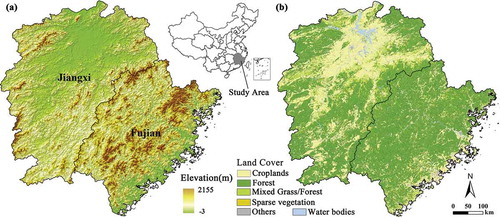
Based on the hypothesis that the influence of climate change on vegetation growth cycles should be measurable in a sensitive system such as mountainous regions (Cunha and Richter 2014), two provinces located in a subtropical mountainous agro-forestry region in southeast China, Fujian (Min for short) and Jiangxi (Gan for short) provinces (Figure 1), were chosen as the study area. The Min-Gan region is located between latitude 23°32′–30°04′N and longitude 113°34′–120°43′E. The topographical features are complex and dominated by mountains and hills, with elevation increased from around zero in the eastern coastal area to 2155 m in the middle north mountains (Figure 1). It has subtropical climate with an annual mean temperature between 16 and 21°C and a yearly precipitation of 920–1934.4 mm. The third largest lake of China, Poyang Lake, is located in the middle-north portion of Jiangxi province. Both Jiangxi and Fujian provinces held the first rank for its proportion of forest cover (over 63%) in 2010 (http://www.stats.gov.cn/tjsj/ndsj). The dominant tree species in Min-Gan region are pine, Eucalyptus, Chinese fir, and some other broad-leaf trees. The province’s major crop types are rice, pachyrhizus, and tobacco leaf.

Figure 1. Location of our study area, its spatial distribution of elevation (a) and land use/land cover (b). Full color available online.

Notes: DBF, ENF, and EBF represent the deciduous broadleaf forests, evergreen needle-leaf forests, and evergreen broadleaf forests, respectively.

2.2. Data sources

The 16-day time series of 250-m moderate resolution imaging spectroradiometer (MODIS) enhanced vegetation index (EVI) product (MOD13Q1) from 2001 to 2011 are utilized. The MODIS EVI product produces a vegetation signal with improved sensitivity in high-biomass regions through the reduction of soil and atmospheric influences (Waring et al. 2006). The DEM data sets are from the Shuttle Radar Topography Mission data with a spatial resolution of 30 m. The meteorological data are obtained from the National Meteorological Information Centre of China during the period 2001–2011. And 300-m GlobCover Land Cover Maps are also utilized (http://globalchange.nsdc.cn) (Figure 1). The meteorological data include semimonthly mean surface air temperature, total precipitation, total sunshine duration, and mean absolute humidity. Co-kriging interpolation is used to establish their spatial distribution images (Chiu, Lin, and Lu 2009). Climatic data from 57 meteorological stations is utilized. First, a trend surface is developed for each climatic variable based on its corresponding determining factors through a regression model. The determining factors/independent variables are selected with reference to related literature (Chiu, Lin, and Lu 2009) and local meteorologists. Topographic effect is critical for temperature and precipitation. Variables of longitude, latitude, and elevation are utilized to construct a linear function for precipitation. For function of temperature, sunshine duration, and humidity, the variables of aspect and slope are also included. The residuals of the trend surface of each climatic variable with reference to meteorological stations are further interpolated by the co-kriging method. And finally, the interpolated images of four climatic variables are achieved based on above procedures.

3. Methodology

The MSSTM framework is provided in Figure 2. First, the original time series of MODIS EVI and four climatic variables are decomposed into multi-temporal scale components through WTs. Second, the relationship between climate factors and vegetation dynamics are also evaluated and specific time-series models are established for each EVI component. Finally, the MSSTM’s ability to explore vegetation dynamics is evaluated. The following sections provide a detailed description of each procedure.

Figure 2. Overview of the MSSTM framework.

Notes: D₁, D₂, D₃, D₄ represent the detailed component at level 1–4, respectively. The A₅ indicates the approximation component for level 5. The D₁, D₂, D₃, D₄, and A₅ roughly correspond to intra-monthly, monthly, bi-monthly, seasonal, and inter-annual variations, respectively.

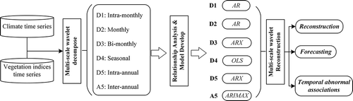
3.1. Multi-temporal scale wavelet decomposition

The WTs provide an efficient tool for processing signals with different frequency components (Daubechies 1990). Through WT, the original time series of MODIS EVI and climate variables are transformed into multi-temporal components. At first level of decomposition, the original signal is decomposed into an Approximation (A₁) and Detailed component (D₁). In the next step, the approximation (A₁) is re-decomposed, and so on. The Detailed components from level 1 to 5 roughly correspond to intra-monthly, monthly, bi-monthly, seasonal, and semiannual variations, respectively: D₁ (<24 days), D₂ (24–48 days), D₃ (48–95 days), D₄ (95–193 days), and D₅ (193–386 days) (Qiu et al. 2013a). The approximation component for level 5, A₅, represents the inter-annual variability (380 days or longer) over the study period. Finally, the original time series of MODIS EVI and four climatic variables are decomposed into intra-monthly, monthly, bi-monthly, seasonal, semiannual, and inter-annual components, respectively. The Meyer orthogonal discrete wavelet is selected for this purpose (Abry 1997). Detailed descriptions can be founded in related references (Qiu et al. 2013a; Martínez and Gilabert 2009).

3.2. Model selection and construction

For each EVI component, the pixel-specific models are developed based on their characteristics and the relationships with climatic variables. When the data are stationary, the temporal auto-regression (AR) models, and autoregressive integrated moving average (ARIMA) models are considered. Otherwise, the autoregressive moving average (MA) model (Box and Jenkins 1976) could generally be utilized. Whether the climatic variables are included within these models or not is depended on their correlations with EVI components. When there are little associations between them, the climatic variables are not contained in the models. Otherwise, the climatic variables are considered in the models. And particularly, when there are very strong correlations between the EVI component and climatic variables, the ordinary linear regression models can be applied.

For each EVI component, the selected model is described as follows. For the detailed component and , the temporal AR models are applied. For the detailed component and , the temporal AR models with external input are utilized. For the detailed component , the ordinary linear regression is employed. For the inter-annual component , an autoregressive integrated MA with exogenous input (ARIMAX) model is adopted. The ARIMAX is an extension of the ARIMA model. In an ARIMA (p,d,q) model, p, q, and d are the numbers of AR, MA parameters, and differences, respectively. The stationarity is checked through Augmented Dickey–Fuller test. For nonstationary time series, it is made to be stationary through differencing. The numbers of temporal AR and MA terms are decided by analyzing the partial autocorrelation function. The best fitting model is determined by the Akaike Information Criterion. The ARIMAX model is applied when climatic variables should be included in the ARIMA model as an additional covariate. For two climatic variables with high colinearity, only one of them can be considered in the model. A spatial model can also be introduced to incorporate the influence from neighbors, topographic and accessibility conditions (not applied in this paper for simplifications).

To evaluate the time lag between climate variables and MODIS EVI, a correlation coefficient is computed between their corresponding time series or half to 4 months’ moving averaged time series. The time lag between EVI and climatic factors could be decided based on the strongest coefficients.

The EVI time-series signal f(t) could be reconstructed from the approximations and detailed components as

(1)

where , , … represent the modeled values of , , … , respectively.

To sum up, the multi-temporal wavelet reconstruction is achieved through summing up the pixel-specific models of each EVI component from intra-monthly to inter-annual scales.

3.3. Implementation and evaluation

The performance assessment of the MSSTM approach was conducted based on its ability of reconstruction and forecasting. The abilities of reconstruction and forecasting are evaluated through the percentages of relative absolute errors (PRAE). The PRAE measures the degree to which the observed and modeled/predicted values are fitted. The percentages of relative absolute errors are defined as the sum of the absolute difference between modeled/predicted and observed values divided by the sum of the observed values of time-series data sets.

(2)

where and stand for the observed and predicted EVI values, respectively, at the ith time step; m is the number of time steps in the modeled period.

The multi-temporal components of time series of vegetation indices and climatic variables could be applied to characterize their complex relationships. The relationships between EVI components and climatic variables are investigated through the Pearson correlation coefficients and their connections of the temporal anomalies. A temporal anomaly is recorded when it is beyond the average value plus/minus 2.0 ratios of standard variance. If a temporal anomaly is simultaneously (or with semi-month’s lag) observed from EVI component and one climatic variable at specific time/scale, it is described a temporal abnormal match (Figure 3).

Figure 3. The calculation process of temporal abnormal associations.

Notes: There were two EVI anomalies. The first EVI anomaly, A₁, was described as a temporal abnormal match, since a temporal anomaly is simultaneously (or with semimonth’s lag) observed from the climatic variable; the second EVI anomaly, A₂, was not.

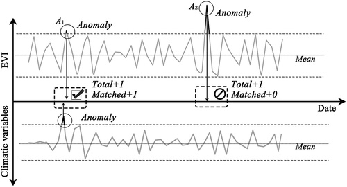
The Temporal Abnormal Association (TAA) is defined as

(3)

where AM stands for the frequency of temporal abnormal match, TE denotes the total number of EVI anomalies for each pixel at one particular temporal scale. The TAA indicates the relative contribution of climatic variables for EVI abnormalities. The TAA are calculated for each specific climatic variable and all four climatic variables, respectively.

The entire procedures of model implementation and evaluation are executed using the Matlab software package (The MathWorks, Natick, Massachusetts, USA).

4. Results and discussions

4.1. Performance assessment of the MSSTM method

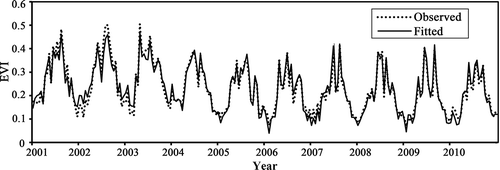
The model performances of reconstruction were evaluated by the spatial distribution map of PRAE (Figure 4). The averaged PRAE of MSSTM method was only 6.65. The MSSTM method achieved significantly smaller PRAE values than those from the ARIMAX method (average PRAE = 16.72). For most pixels, the PRAE from the MSSTM method were less than 11 (Figure 4(a)). However, the PRAE from the ARIMAX were generally greater than 11 (Figure 4(b)). One randomly selected pixel was selected to illustrate the fitting effects of the MSSTM method compared with observed data sets (Figure 5). The MSSTM method provided good estimates of the peaks and valleys of the observed EVI, which were critical for phenological and related studies.

Figure 4. Comparison of percentages of relative absolute errors from the MSSTM (a) and ARIMAX (b) models. Full color available online.

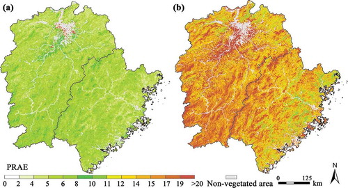
Figure 5. Comparison between observed and fitted EVI through MSSTM method during 2001–2010.

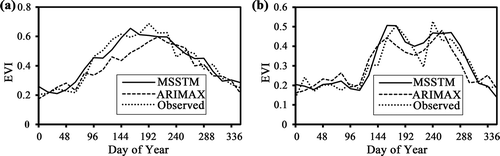
The model performances of predictive capability were also assessed by the PRAE. Two hundreds of random selected agricultural and forest sites were applied. The MSSTM model was first trained with the data during the period 2001–2010 and then performed to forecast EVI time series in 2011. The predicted EVI values by the proposed MSSTM and ARIMAX methods from one forest and one agricultural site were provided (Figure 6). Compared with the ARIMAX model, the MSSTM method provided a better estimation of EVI. The ARIMAX model underestimated during the vegetation growing stage for forest sites and delivered biased estimated peaks for vegetation with multiple growth cycles (e.g. double crops). The averaged PRAE from ARIMAX method was 20.77. Comparatively, significantly smaller (p value < 0.005) averaged PRAE value was obtained from the MSSTM method (17.15).

Figure 6. Comparison between observed and predicted in 2011 for ARIMAX and MSSTM from one forest (a) and one agricultural site (b).

The better performance of MSSTM than ARIMAX was derived from both the algorithm characteristics and the specific environmental conditions of a target area. Through reconstructing the EVI from multiple wavelet components, the MSSTM approach could take full advantages of the unique characteristics of each wavelet component and its corresponding model was selected. Through selecting specific model and its corresponding exogenous inputs from climatic variables at each scale, the MSSTM approach could efficiently cope with the specific environmental conditions of a target area.

The wavelet-based methods have been successfully utilized in characterizing multi-scale patterns of vegetation dynamics (Yang et al. 2012; Martínez and Gilabert 2009; Singh et al. 2012; Qiu et al. 2014b, 2013a). The proposed MSSTM method took advantage of the multi-scale wavelet decomposition and reconstruction framework. The MSSTM method summed up the approximations and necessary detailed components estimated from proper time-series models. Through incorporating their temporal characteristics and associations with climate factors, the MSSTM method was proved to be suitable for reconstructing and forecasting EVI time series.

4.2. Multi-temporal scale vegetation dynamic patterns under the influence of four climate variables

The best overall correlation can be observed between EVI and precipitation with about 1 month’s (two 16-day composites) lag. Therefore their correlation coefficients were calculated with two composites’ lag. From intra-monthly to inter-annual scale, the correlation coefficients between EVI components and four climatic variables were computed through a per-pixel strategy. Totally 24 images of their correlation coefficients were acquired. At smaller scale, the histogram images of their correlation coefficients were provided in Figure 7. At intra-monthly and monthly scales, their correlation coefficients were very low and commonly within [−0.1,0.1] (Figure 7). Their correlation coefficients at larger scales (bi-monthly, seasonal, and intra-annual scales) were analyzed at different altitudinal gradients (0–100 m, 100–200 m, 200–400 m, 400–700 m, and above 700 m) for agricultural and forest vegetation, respectively (Figure 8). Their correlation coefficients might change from strong negative to positive, depending on the analyzed temporal scale, altitudinal gradients, and different climatic variables.

Figure 7. Histogram of correlation coefficients between climatic variables and EVI components at intra-monthly (D₁) and monthly (D₂) scales.

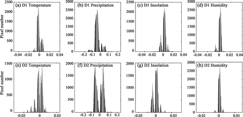
Figure 8. Boxplots of correlation coefficients of meteorological parameters as a function of elevation for agricultural crop (a, c, e) and forest (b, d, f) vegetation at bi-monthly (D₃), seasonal (D₄) and intra-annual (A₅) scales. The line in the center of the box refers to the medium value of the population, while inside the box lie the 50% of the observations (from the 25th to 75th percentile). Full color available online.

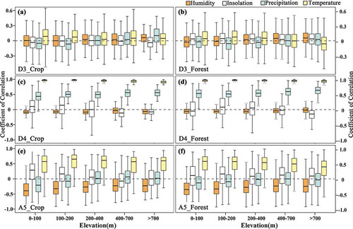
At intra-annual scales, the correlation coefficients of meteorological variables on vegetation dynamics generally increased from intra-monthly, monthly, and bi-monthly to seasonal scales (Figures 7 and 8). Compared with those from intra-monthly and monthly scales, their correlations at bi-monthly scale (D₃) were slightly stronger but their interquartile ranges were still commonly within [−0.2,0.2]. Nevertheless, at seasonal scale, there were strong correlations between EVI and climatic variables (Figure 8), particularly the temperature (averaged correlation coefficients 0.92) and precipitation (averaged correlation coefficients 0.52). As the altitude increased, the linear correlations between EVI and temperature slightly decreased: the averaged value was 0.9625, 0.9509, 0.9386, and 0.9219 for altitudinal bands of below 0–100, 100–200, 200–400, 400–700, and above 700 m, respectively. However, the correlations between EVI and precipitation gently increased with altitude at seasonal scale: the averaged value was 0.4612, 0.5119, 0.5297, 0.5813, and 0.621 for altitudinal bands of 0–100, 100–200, 200–400, 400–700, and above 700 m, respectively.

At intra-annual scales, the associations between EVI and precipitation at seasonal scale also differed among different vegetation types. There slight stronger EVI–precipitation correlations from the forest vegetation (averaged 0.56) compared to those from croplands (averaged 0.45). Differed from the temperature and precipitation, uncertain relationship was observed between EVI and sunshine duration (insolation) at seasonal scale: the correlations coefficients varied from negative to positive and its amplitudes generally decreased with altitudinal gradients: the averaged value was 0.257, 0.294, 0.246, 0.1732, and 0.1879 for altitudinal bands of 0–100, 100–200, 200–400, 400–700, and above 700 m, respectively. There were no close linear correlations between EVI and humidity even at seasonal scale.

At inter-annual scale (A₅), positive relationships were also generally observed between temperature and EVI, but less than those at seasonal scale. The precipitation and humidity generally had slightly negative or no obvious relationship with vegetation dynamics. There was also somewhat positive correlation between sunshine duration and EVI at inter-annual scale for forest vegetation at lower altitudes (below 100 m). It suggested limited influence of climatic variables such as precipitation and humidity variations in humid regions at longer temporal scales.

Considerable recent studies demonstrated that the detailed relationships between vegetation activities and climate factors might be more complex and highly nonlinear (Herdianto et al. 2013; Gessner et al. 2013). For example, a study in North American continent confirmed that the normalized difference vegetation index (NDVI)–temperature correlation was generally positive when energy was the limiting factor (Karnieli et al. 2010). Another study in forested catchment in Korea indicated that the EVI–temperature relationship exhibited a threshold above which the rate of EVI increase changed significantly (Herdianto et al. 2013). Chang et al. (2014) found that EVI was positively related to temperature and precipitation at monthly scale but not at annual scale, through a case study in Taiwan, Southeast Asia. Horion et al. (2013) showed that meteorological variables highly correlated with NDVI at yearly scale were not necessarily associated when considering different periods of the growing season, based on 12 regions characterized by dominant and stable cropland or grassland covers in Europe and Africa.

This paper provided knowledge on vegetation–climate associations covering from intra-monthly, monthly, bi-monthly, seasonal scales to inter-annual scale through exploring the complex agroforestry vegetation dynamics in subtropical mountains regions based on the proposed MSSTM method. First, at seasonal scale, this paper confirmed the strong positive relationship between vegetation dynamics and climatic variables (particularly the temperature). Although their strong associations at seasonal scale were already indicated in literature due to their synchronous seasonal patterns (Yang et al. 2012; Qiu et al. 2014b), this study further revealed that the seasonal patterns varied with altitudes and vegetation.

Second, at inter-annual scale, this paper found that vegetation dynamics were obviously influenced by temperature. Slightly correlations could be observed between EVI and other climatic variables such as precipitation, sunshine duration, and humidity for some pixels. The correlation coefficients might vary from negative to positive among different altitudes and climatic variables. These findings obviously differed with related studies (Chang et al. 2014). The inconsistency might due to the reason that the mean value of all pixels of each vegetation type was applied in Chang et al.’s (2014) study. Through a per-pixel strategy, our study exposed the strong spatial heterogeneity as regards to the vegetation–climate relationships. The averaged values in Chang et al.’s (2014) study might conceal the variations from negative-to-positive correlation coefficients.

Third, at intra-seasonal scales, this paper revealed that there were no strong linear relationships between vegetation dynamics and four climatic variables (temperature, precipitation, sunshine duration, and humidity). Climatic variables highly correlated with EVI at one scale were not necessarily associated at other scales, which conformed to other related studies (Horion et al. 2013; Yang et al. 2012; Qiu et al. 2014b). This paper enriched our knowledge of the complex EVI–climate relationships from monthly to inter-annual scales through incorporation variables of sunshine duration and humidity.

4.3. The sensibility of vegetation anomalies to climate changes

To better understand the intra-annual variation of the climatic influence on vegetation growth at smaller scales, we analyzed how smaller scales’ (intra-monthly, monthly, and bi-monthly) anomalies were temporal associated. The TAA between EVI components and climatic variables were calculated through a per-pixel strategy. The spatial distribution maps of TAA for climatic variables (temperature, precipitation, and sunshine durations) at intra-monthly, monthly, and bi-monthly scales were provided in Figure 9.

Figure 9. The spatial distribution map of TAA of four climatic variables at intra-monthly (a), monthly (b) and bi-monthly (c) scales. Full color available online.

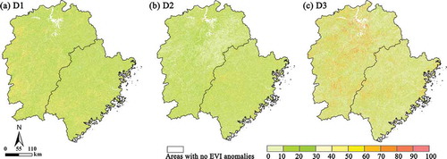
Despite the low correlation coefficients at intra-seasonal scales, over one-fifth of EVI anomalies were associated with temporal anomalies of climatic variables. The average TAA of these climatic variables was 24.46, 19.82, and 20.73 at intra-monthly, monthly, and bi-monthly scales, respectively. It indicated that considerable EVI anomalies were attributed to climatic anomalies. Among these four climatic variables, the precipitation played the most important role for EVI anomalies. The average TAA of precipitation was 17.39, 10.52, and 9.15 at intra-monthly, monthly, and bi-monthly scales, respectively. The sunshine duration ranked the second responsibility for EVI anomalies. Despite the strong linear correlations with EVI at seasonal scale, the temperature played less important role for EVI anomalies compared with precipitation and sunshine duration.

More research attentions should be paid to develop integrated models that are suitable to multi-temporal scale vegetation system in order to reflect both long- and short-term effects under various disturbances (You, Liu, and Zhang 2015). Our proposed MSSTM method could be applied for this purpose. Due to the complexity and nonlinear vegetation–climate relationship, growing research interests focused on the anomaly/disturbance analysis of vegetation dynamics (Gessner et al. 2013; Kim 2013). These studies revealed that vegetation anomalies were subscribed to disturbances from climatic process. For example, a study in the northern Arizona ecosystem found EVI anomalies were likely sensitive to the amount of rainfall and the higher elevation areas showed slow recovery (Kim 2013). Another study in central Asia also showed that vegetation development was sensible to precipitation anomalies for nearly 80% of study area (Gessner et al. 2013). The start dates significantly advanced and end dates remarkably delayed during anomalously warm years in subtropical mountain and hill region (Qiu et al. 2013b).

Despite the increasing interest in vegetation anomalies, few studies concentrated on the anomaly connections with various climatic variables from intra-monthly to bi-monthly scales. Although the sensitivity of EVI anomalies to the precipitation was confirmed in recent studies (Kim 2013; Gessner et al. 2013), the relative roles of precipitation as well as temperature, humidity, and sunshine duration were fairly unknown. As regards to the third research question proposed in the introduction section, this paper provided the following scientific findings under the proposed multi-temporal scale modeling framework through the TAA analysis. Among four climatic variables, despite no obvious linear correlations, precipitation and sunshine duration are primarily responsible for the vegetation dynamics anomalies from intra-monthly to bi-monthly scales. Regardless of the particularly strong linear correlations with vegetation dynamics at seasonal scale, the temperature played less important role for the intra-seasonal EVI anomalies than precipitation and sunshine duration.

Therefore, this paper provided knowledge on vegetation–climate associations covering from intra-monthly, monthly, bi-monthly, seasonal scales to inter-annual scale through exploring the complex agroforestry vegetation dynamics in subtropical mountains regions based on the proposed MSSTM method.

4.4. Potential applications of MSSTM method

The proposed MSSTM method is proved to be efficient in characterizing the complex vegetation dynamics patterns under global climate change through its applications in subtropical mountainous agro-forestry ecosystem. There are also some other potential applications for the established multi-temporal scale spatiotemporal explicit modeling approaches. Due to its capability of reconstructing and foresting, the proposed MSSTM method can be applied to develop spatiotemporal data fusion method. Another significant application is to establish time-series classification method for vegetation/land cover change.

Several efficient continuous vegetation/land cover change mapping methods have recently been established through time-series-based approaches (Zhu and Woodcock 2014; Setiawan and Yoshino 2014). Zhu and Woodcock (2014) proposed a time-series model for the purpose of continuous change detection and classification (CCDC). The CCDC model had components of seasonality, trend and break estimates surface reflectance and brightness temperature (Zhu and Woodcock 2014). Similarly, there was also components of seasonal and inter-annual (trend) scales in the MSSTM model. However, the ordinary linear regression (OLS) model was applied for estimating the seasonal component, instead of the Sin() and Cos() functions utilized in the CCDC model.

In CCDC model (Zhu and Woodcock 2014), the coefficients from the time-series model and the root mean square error from model estimation are applied as input for classifier. Correspondingly, the coefficients and model residuals in the MSSTM method could also be utilized for classifications. The vegetation response to climate changes can also be incorporated for vegetation/land cover identification through the MSSTM approach. Furthermore, by the MSSTM approach, the multi-temporal EVI components themselves and their relative variability could also be exploited for vegetation/land-cover mapping. The variations of different multi-temporal EVI components provided significant information on vegetation types (Qiu et al. 2013a). For example, roughly equal wavelet variance was observed from monthly to semiannual scales from multiple cropping croplands (Qiu et al. 2013a). The multi-temporal EVI components obtained through wavelet transforms were proved to be efficient in vegetation/land-cover identifications as parameters inputs (Qiu et al. 2014a; Singh et al. 2012; Qiu et al. 2013a).

The differences between the observed and predicted are utilized as an indication for change detection in CCDC model (Zhu and Woodcock 2014). When land-cover change occurred on a pixel, there will be a gap between the predicted and observed values. Correspondingly, in the MSSTM method, we could identify land-cover change through the model residuals. It is possible to distinguish actual land-use change based on land-cover dynamics through characterizing temporal vegetation dynamics (Setiawan and Yoshino 2014). Nevertheless, this paper only explored vegetation dynamics patterns under global climate change through proposing a multi-scale spatiotemporal modeling approach. Potential applications of MSSTM method will be carried out in the future work.

4.5. Possible influences from data uncertainties and future work

Given that there is a growing interest in characterizing vegetation dynamics through spatial and temporal explicit time-series approaches, appropriate modeling methods designed particularly for this purpose are limited. This paper proposed a MSSTM approach which proved to be efficient in vegetation indices reconstructing and forecasting. In addition, it provided full knowledge on the relationships between vegetation dynamics and climate variables at multi-temporal scales. The relative role of four variables, the linear correlations and anomalies associations, were analyzed from intra-monthly, monthly, bi-monthly, seasonal scales to inter-annual scales. The 16-day composite MODIS EVI time-series data sets and the interpolated climatic data sets were utilized. Nevertheless, the MODIS EVI time-series data sets might be disturbed by cloud cover or other noise (Qiu et al. 2013a). It could be inferred that a large proportion of EVI anomalies at smaller temporal scales might be introduced by data noise. And uncertainties might also be introduced during the spatial interpolation process of climatic variables.

In order to evaluate the influence of data uncertainties introduced by cloud contaminations, this paper identified each MODIS EVI data composite contaminated by cloud contaminations with reference to the Quality layers during the study period 2001–2011, and calculated frequency of cloud contamination durations during the study period. Most pixels (98.25%) were associated with the frequency of cloud contamination durations of no more than three continuous data composites (48 days). Considering the frequency of cloud contamination duration and the wavelet components, the detailed components D₁ (<24 days) and D₂ (24–48 days) would likely be disturbed by cloud contaminations. In order to evaluate the influence of each wavelet component on model performance of reconstruction, we computed their normalized wavelet-variance (Qiu et al. 2013a). The average percentage of the normalized wavelet variance for detailed component D₁ and D₂ is 5.65% and 4.86%, respectively. Therefore, the detailed component D₁ and D₂ would have limited influence on the model reconstruction. Regarding possible influence of cloud contaminations on TAA at smaller scales, this study re-conducted the experiments through discarding the data composites with cloud contaminations. There were no fundamental differences between them. The average TAA of these climatic variables changed to 18.99, 17.65, and 19.73 at intra-monthly, monthly, and bi-monthly scales, respectively. The average TAA of these climatic variables slightly decreased, particularly at smaller scale. It is because the TAA at intra-monthly scale probably introduced by cloud contaminations were discarded.

Due to the limitations of MODIS collections 5 (e.g. BRDF effects), this paper computed the difference between MODIS collections 5 and the new MODIS Collection 6 products in order to evaluate the influence of data uncertainties. Their absolute differences (EVI_MODIS5 − EVI_MODIS6) and the comparative differences (100 × ｜EVI_MODIS5 − EVI_MODIS6｜/EVI_MODIS6) were calculated (figure below). Most pixels (97.66%) were observed with the absolute differences of less than 0.03. The EVI values from MODIS 5 were considerably greater than those from MODIS 6. The averaged absolute difference between these two data sets was 0.0157 over the study area. Regarding the comparative differences, pixels with relatively larger values primarily located in the non-vegetated areas. The comparative difference of croplands, forests and non-vegetation was 8.7107, 8.9429, and 10.7096, respectively. Specifically, 96.11% croplands and 98.86% forests pixels were examined with absolute difference of less than 15. The proposed MSSTM approach and its applications based on MODIS collections 5 was still valuable and it could further apply to these new available data sets.

Future work could be conducted on (1) in order to incorporate the uncertainties from the interpolation process of climatic data, spatial explicit climatic map derived from remote sensing images could be employed. (2) Other methods of anomaly analysis could be applied the complex vegetation response to climatic variability in terms of sensibility and resilience to extreme events such as drought or frost. (3) Further applications of the proposed MSSTM to other regions are necessary to verify the reliability. (4) It was also necessary to further evaluate its ability of forecasting and exploring the implications of model fitness and model residuals. For example, could the model residuals be associated with climatic abnormalities or vegetation disturbance? (5) Further applications for designing new automatic detection method of land-cover change could be made based on the predictive capability and other model parameters.

5. Conclusions

The proposed MSSTM was efficient in characterizing and forecasting spatiotemporal vegetation dynamics through developing pixel and scale specific time-series models based on its characteristics and connections with climatic variables. The MSSTM approach achieved much less averaged PRAE for reconstruction than those directly from ARIMAX method. The MSSTM was flexible to incorporate proper time-series models and influences from extra-variables and neighborhoods. Through its application to a subtropical mountainous and hilly region, four research questions proposed in the introduction section could be addressed.

1. The relationship between climate and vegetation dynamics vary at inter-annual, seasonal, and intra-seasonal scales. Climatic variables are highly positively correlated with EVI at seasonal scale, particularly with the temperature and precipitation. But their correlations coefficients between EVI and these two climatic variables were much less at inter-annual scale and there were no strong linear correlations between them at intra-seasonal scales. Differed from the temperature and precipitation, less obvious relationships was observed between EVI and sunshine duration at seasonal scale: the correlations coefficients varied from negative to positive. There were somewhat positive correlations between EVI and sunshine duration at inter-annual scale. However, there were no strong linear correlations between EVI and humidity from intra-seasonal to inter-annual scales.

2. The EVI–climatic association is not consistent among different vegetation/land-use types and across various altitudinal gradients. For example, the EVI–temperature correlations decreased but the EVI–temperature connections increased with altitudes at seasonal scale. Slightly stronger correlations between EVI and precipitation were obtained in forest vegetation instead of the croplands. The correlations coefficients between EVI and sunshine duration generally decreased with altitudinal gradients.

3. The sunshine duration, together with precipitation, was principally responsible for considerable EVI anomalies at intra-seasonal scales. The variable of humidity had limited influence on vegetation dynamics in humid regions.

4. Through a per-pixel and scale-specific strategy, this paper indicated the EVI–climate relationships are definitely not consistent among different scales. The proposed MSSTM approach can certainly be employed to characterize the complex vegetation dynamics in other regions. The model parameters will be very valuable for continuous vegetation monitoring, analysis, and classifications.

Acknowledgment

We are very grateful for the thorough and constructive comments from the reviewers of the manuscript. We also acknowledge the funding provided by National Natural Science Foundation of China(41471362).

Disclosure statement

No potential conflict of interest was reported by the authors.

Additional information

Funding

This work was supported by the National Natural Science Foundation of China: [Grant Number 41471362].

References

- Abry, P. 1997. “Ondelettes et turbulence.” In Multiresolutions, algorithmes de decomposition, invariance dechelles, edited by Diderot, 268. Paris: Diderot éd. Press.
- Baynard, C. W. 2013. “Remote Sensing Applications: Beyond Land-Use and Land-Cover Change.” Advances in Remote Sensing 2 (3): 228–241. doi:10.4236/ars.2013.23025.
- Box, G. E. P., and G. M. Jenkins. 1976. Time Series Analysis: Forecasting and Control. revised ed. San Francisco: Holden-Day.
- Chang, C.-T., S.-F. Wang, M. A. Vadeboncoeur, and T.-C. Lin. 2014. “Relating Vegetation Dynamics to Temperature and Precipitation at Monthly and Annual Time Scales in Taiwan Using MODIS Vegetation Indices.” International Journal of Remote Sensing 35 (2): 598–620. doi:10.1080/01431161.2013.871593.
- Chiu, C.-A., P.-H. Lin, and K.-C. Lu. 2009. “GIS-Based Tests for Quality Control of Meteorological Data and Spatial Interpolation of Climate Data: A Case Study in Mountainous Taiwan.” Mountain Research and Development 29 (4): 339–349. doi:10.1659/mrd.00030.
- Cuba, N., J. Rogan, Z. Christman, C. A. Williams, L. C. Schneider, D. Lawrence, and M. Millones. 2013. “Modelling Dry Season Deciduousness in Mexican Yucatán Forest Using MODIS EVI Data (2000–2011).” GIScience & Remote Sensing 50 (1): 26–49. doi:10.1080/15481603.2013.778559.
- Cunha, M., and C. Richter. 2014. “A Time-frequency Analysis on the Impact of Climate Variability on Semi-Natural Mountain Meadows.” IEEE Transactions on Geoscience and Remote Sensing 52 (10): 6156–6164. doi:10.1109/TGRS.2013.2295321.
- Daubechies, I. 1990. “The Wavelet Transform, Time-Frequency Localization and Signal Analysis.” IEEE Transactions on Information Theory 36 (5): 961–1005. doi:10.1109/18.57199.
- Ding, M., Q. Chen, L. Li, Y. Zhang, Z. Wang, L. Liu, and X. Sun. 2015. “Temperature Dependence of Variations in the End of the Growing Season from 1982 to 2012 on the Qinghai–Tibetan Plateau.” GIScience & Remote Sensing 1–17. doi:10.1080/15481603.2015.1120371.
- Gessner, U., V. Naeimi, I. Klein, C. Kuenzer, D. Klein, and S. Dech. 2013. “The Relationship Between Precipitation Anomalies and Satellite-Derived Vegetation Activity in Central Asia.” Global and Planetary Change 110: 74–87. doi:10.1016/j.gloplacha.2012.09.007.
- Hawinkel, P., E. Swinnen, S. Lhermitte, B. Verbist, J. Van Orshoven, and B. Muys. 2015. “A Time Series Processing Tool to Extract Climate-Driven Interannual Vegetation Dynamics Using Ensemble Empirical Mode Decomposition (EEMD).” Remote Sensing of Environment 169: 375–389. doi:10.1016/j.rse.2015.08.024.
- Herdianto, R., K. Paik, N. A. Coles, and K. Smettem. 2013. “Transitional Responses of Vegetation Activities to Temperature Variations: Insights Obtained from a Forested Catchment in Korea.” Journal of Hydrology 484 (0): 86–95. doi:10.1016/j.jhydrol.2013.01.011.
- Horion, S., Y. Cornet, M. Erpicum, and B. Tychon. 2013. “Studying Interactions Between Climate Variability and Vegetation Dynamic Using a Phenology Based Approach.” International Journal of Applied Earth Observation and Geoinformation 20 (1): 20–32. doi:10.1016/j.jag.2011.12.010.
- Huesca, M., J. Litago, S. Merino-de-Miguel, V. Cicuendez-López-Ocañaa, and A. Palacios-Orueta. 2014. “Modeling and Forecasting MODIS-Based Fire Potential Index on a Pixel Basis Using Time Series Models.” International Journal of Applied Earth Observation and Geoinformation 26: 363–376. doi:10.1016/j.jag.2013.09.003.
- Jamali, S., P. Jönsson, L. Eklundh, J. Ardö, and J. Seaquist. 2015. “Detecting Changes in Vegetation Trends Using Time Series Segmentation.” Remote Sensing of Environment 156: 182–195. doi:10.1016/j.rse.2014.09.010.
- Karnieli, A., N. Agam, R. T. Pinker, M. Anderson, M. L. Imhoff, G. G. Gutman, N. Panov, and A. Goldberg. 2010. “Use of NDVI and Land Surface Temperature for Drought Assessment: Merits and Limitations.” Journal of Climate 23 (3): 618–633. doi:10.1175/2009JCLI2900.1.
- Keane, R. E., D. A. Donald McKenzie, E. A. Falk, H. Smithwick, C. Miller, and L.-K. B. Kellogg. 2015. “Representing Climate, Disturbance, and Vegetation Interactions in Landscape Models.” Ecological Modelling 309–310 (309): 33–47. doi:10.1016/j.ecolmodel.2015.04.009.
- Kim, Y. 2013. “Drought and Elevation Effects on MODIS Vegetation Indices in Northern Arizona Ecosystems.” International Journal of Remote Sensing 34 (14): 4889–4899. doi:10.1080/2150704X.2013.781700.
- Krishnaswamy, J., R. John, and S. Joseph. 2014. “Consistent Response of Vegetation Dynamics to Recent Climate Change in Tropical Mountain Regions.” Global Change Biology 20 (1): 203–215. doi:10.1111/gcb.12362.
- Martínez, B., and M. A. Gilabert. 2009. “Vegetation Dynamics from NDVI Time Series Analysis Using the Wavelet Transform.” Remote Sensing of Environment 113 (9): 1823–1842. doi:10.1016/j.rse.2009.04.016.
- Nemani, R. R., C. D. Keeling, H. Hashimoto, W. M. Jolly, S. C. Piper, C. J. Tucker, R. B. Myneni, and S. W. Running. 2003. “Climate-Driven Increases in Global Terrestrial Net Primary Production from 1982 to 1999.” Science 300 (5625): 1560–1563. doi:10.1126/science.1082750.
- Qiu, B. W., Z. L. Fan, M. Zhong, Z. H. Tang, and C. C. Chen. 2014a. “A New Approach for Crop Identification with Wavelet Variance and JM Distance.” Environmental Monitoring and Assessment 186: 7929–7940. doi:10.1007/s11769-013-0649-y.
- Qiu, B. W., W. J. Li, M. Zhong, Z. H. Tang, and C. C. Chen. 2014b. “Spatiotemporal Analysis of Vegetation Variability and Its Relationship with Climate Change in China.” Geo-Spatial Information Science 17 (3): 170–180. doi:10.1080/10095020.2014.959095.
- Qiu, B. W., C. Y. Zeng, Z. H. Tang, and C. C. Chen. 2013a. “Characterizing Spatiotemporal Non-Stationarity in Vegetation Dynamics in China Using MODIS EVI Dataset.” Journal of Environmental Monitoring and Assessment 185 (11): 9019–9035. doi:10.1007/s10661-013-3231-2.
- Qiu, B. W., M. Zhong, Z. H. Tang, and C. C. Chen. 2013b. “Spatiotemporal Variability of Vegetation Phenology with Reference to Altitude and Climate in the Subtropical Mountain and Hill Region, China.” Chinese Science Bulletin 58 (23): 2883–2892. doi:10.1007/s11434-013-5847-6.
- Setiawan, Y., and K. Yoshino. 2014. “Detecting Land-Use Change from Seasonal Vegetation Dynamics on Regional Scale with MODIS EVI 250-M Time-Series Imagery.” Journal of Land Use Science 9 (3): 304–330. doi:10.1080/1747423X.2013.786151.
- Singh, A., R. Dutta, A. Stein, and R. M. Bhagat. 2012. “A Wavelet-Based Approach for Monitoring Plantation Crops (Tea: Camellia Sinensis) in North East India.” International Journal of Remote Sensing 33 (16): 4982–5008.
- Song, Y., and M. Ma. 2011. “A Statistical Analysis of the Relationship Between Climatic Factors and the Normalized Difference Vegetation Index in China.” International Journal of Remote Sensing 32 (14): 3947–3965. doi:10.1080/01431161003801336.
- Wang, H., D. Liu, H. Lin, A. Montenegro, and X. Zhu. 2015. “NDVI and Vegetation Phenology Dynamics Under the Influence of Sunshine Duration on the Tibetan Plateau.” International Journal of Climatology 35 (5): 687–698. doi:10.1002/joc.4013.
- Waring, R. H., N. C. Coops, W. Fan, and J. M. Nightingale. 2006. “MODIS Enhanced Vegetation Index Predicts Tree Species Richness Across Forested Ecoregions in the Contiguous USA.” Remote Sensing of Environment 103 (2): 218–226. doi:10.1016/j.rse.2006.05.007.
- Yang, Y., J. Xu, Y. Hong, and G. Lv. 2012. “The Dynamic of Vegetation Coverage and its Response to Climate Factors in Inner Mongolia, China.” Stochastic Environmental Research and Risk Assessment 26 (3): 357–373. doi:10.1007/s00477-011-0481-9.
- You, X., J. Liu, and L. Zhang. 2015. “Ecological Modeling of Riparian Vegetation Under Disturbances: A Review.” Ecological Modelling 318: 293–300. doi:10.1016/j.ecolmodel.2015.07.002.
- Yuan, F., C. Wang, and M. Mitchell. 2014. “Spatial Patterns of Land Surface Phenology Relative to Monthly Climate Variations: US Great Plains.” GIScience & Remote Sensing 51 (1): 30–50. doi:10.1080/15481603.2014.883210.
- Zhu, Z., and C. E. Woodcock. 2014. “Continuous Change Detection and Classification of Land Cover Using All Available Landsat Data.” Remote Sensing of Environment 144 (0): 152–171. doi:10.1016/j.rse.2014.01.011.
- Zhu, Z., C. E. Woodcock, C. Holden, and Z. Yang. 2015. “Generating Synthetic Landsat Images Based on All Available Landsat Data: Predicting Landsat Surface Reflectance at any Given Time.” Remote Sensing of Environment 162: 67–83. doi:10.1016/j.rse.2015.02.009.