Application of MK-PRISM for interpolation of wind speed and comparison with co-kriging in South Korea

Abstract

The spatial distribution of wind speed is important information required to understand climate-related regional phenomena. This paper presents the Modified Korean Parameter-elevation Regression on Independent Slopes Model (MK-PRISM) as a method for spatial interpolation of monthly wind speeds. A database of gridded monthly mean wind speeds with a spatial resolution of 1 km for the period of March 2011–February 2014 is constructed by MK-PRISM. Wind speed observation data collected from the 529 to 641 meteorological stations in South Korea were utilized as the input data for interpolation. The wind speed distribution estimated by co-kriging is used for comparison with the MK-PRISM results. Research demonstrates that the efficiency difference between the two models, MK-PRISM and co-kriging, is insignificant. The Kling and Gupta efficiencies of both models were 0.68-0.78 and the root mean square errors (RMSEs) were 0.44-0.68 m/s. The spatial distribution of wind speeds, however, differs between MK-PRISM and co-kriging, which can be considered a reflection of the influence of topographic features such as terrain convexity, aspect, and coastal proximity. MK-PRISM can perform more appropriately to represent the phenomena where similar wind speeds appear continuously along ridges and coastlines. This suggests that a knowledge-based approach that considers topographic features can be successfully applied to the interpolation of monthly or seasonal wind speeds, similar to temperature and precipitation. The wind speed distribution generated by MK-PRISM can be utilized as important data for different geographical studies.

Keywords:

• wind speed
• interpolation
• MK-PRISM
• co-kriging
• South Korea

1. Introduction

Gridded climate data with regular spacing have been widely used in various studies including ecological modeling, hydrological modeling, and climate change impact assessment (Cooke et al. 2012; Pianalto and Yool 2013). The spatial distribution of wind speed is especially important for evapotranspiration estimation (Park 2009; Choi, Cooke, and Stevens 2009), verification of gridded numerical weather prediction forecast fields (Jiménez et al. 2010), and wind resource assessment (Archer and Jacobson 2013).

When considering irregular networks, gridded climate data can be generated through numerical modeling (Skamarock et al. 2005; Kang, Cha, and Lee 2005) or statistical interpolation (Shin et al. 2008; Beier et al. 2011). Gridded climate data can be obtained by remote sensing (Hill 2013; Rhee, Park, and Lu 2014). Statistical interpolation has been used to complement the data gaps caused by numerous conditions such as cloud or sensor noise (Reynolds et al. 2007). The majority of the wind speed mapping approaches is supported by numerical models. Therefore, with the recent increase in weather stations, studies that utilize statistical interpolation of gridded wind speed data are increasing (Robert, Foresti, and Kanevski 2013).

In previous studies, inverse distance weighting (IDW) and kriging methods have been used in wind speed interpolation and kriging has been widely used (Kim, Youn, and Kim 2010; Phillips and Mark, 1996; Cellura et al. 2008). According to Luo, Taylor, and Parker (2008), kriging is limited in its ability to appropriately reproduce wind speeds in mountain and coastal areas because weather stations are typically located in areas with low topography or around cities. Co-kriging has been utilized to overcome such limitations (Luo, Taylor, and Parker 2008) and there have been other studies using artificial neural network (ANN) (Fadare 2010; Philippopoulos and Deligiorgi 2012).

Statistical interpolation methods can be classified into two types. The first type addresses geographical coordinates (X, Y, Z) such as IDW and kriging techniques. The second type includes methods that can consider topographic features such as co-kriging and ANN methods. They generally use a digital elevation model as the secondary variable.

Parameter-elevation Regressions on Independent Slopes Model (PRISM), proposed by Daly, Neilson, and Phillips (1994), is also a method that can consider the effects of topography when interpolating climate data. PRISM determines the value of an unknown cell by considering the effects of variables such as elevation, topographic facet, and coastal proximity (Daly et al. 2008). PRISM is a methodology that was developed after recognizing that IDW and kriging had difficulty reproducing orographic precipitation and that co-kriging could not reproduce the rain shadow effect (Daly, Neilson, and Phillips 1994). This method not only effectively reproduces the rain shadow effect of precipitation but can also reproduce orographic precipitation (Simpson et al. 2005). In South Korea, Modified Korean-PRISM (MK-PRISM) was developed by Kim et al. (2012). It is a version where the variables of PRISM were simplified and successfully applied to generate climate data with a spatial resolution of 1 km (Park and Kim 2013).

PRISM should be applicable to the interpolation of wind speed owing to the use of various topographic features. However, there has never been a case where PRISM has been applied to the interpolation of wind speed. Further, comparative studies on wind speed interpolation methods that can consider the effects of topography are lacking.

The first objective of this paper is to address the question: “Can MK-PRISM be applied to wind speed interpolation?” The second objective is to contrast the wind speed data generated by the two interpolation methods (MK-PRISM and co-kriging) that can consider the effects of topography. Hence, in this study, the structure of MK-PRISM is modified and applied to wind speed interpolation for Korea. Then, the results are compared with the co-kriging interpolation outcomes.

2. Materials and methods

2.1. Study process

The research was conducted according to the procedure illustrated in Figure 1. The measured monthly wind speeds were obtained from the National Weather Service and used as input data for interpolation. The data were also used to calculate the seasonal average wind speeds, which in turn were applied to analyze the spatial characteristics of wind speed. This analysis result was used to modify MK-PRISM for wind speed interpolation.

Figure 1. Study process flow chart.

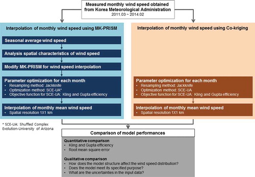
The parameter values of MK-PRISM and co-kriging were determined through an optimization method, the shuffled complex evolution method developed at the University of Arizona (SCE-UA: Duan, Sorooshian, and Gupta 1992). The monthly mean wind speed was used for parameter optimization. This parameter value was used to generate the gridded monthly wind speed data with 1-km spatial resolution.

The interpolation results of MK-PRISM and co-kriging were evaluated via qualitative and quantitative methods. Kling-Gupta efficiency (KGE) and root mean square error (RMSE) were employed for the quantitative evaluation. KGE is a useful criterion for evaluating model performance when the measured and estimated values have a 1:1 relationship (Gupta et al. 2009). In the qualitative evaluation, the manner that each method reproduced wind speed distribution was compared using seasonal average wind speed distribution maps.

2.2. Study area and data set

The study area was the country of South Korea (Figure 2). South Korea is surrounded by the sea on three sides. The Taebaek Mountain range is located in a north–south direction in the east and the Sobaek Mountain range diverges from the center of the Taebaek range extending in a northeast–southwest direction. Western Korea has a relatively low topography and consists primarily of plains.

Figure 2. The study area and locations of stations (February 2014) used in this study.

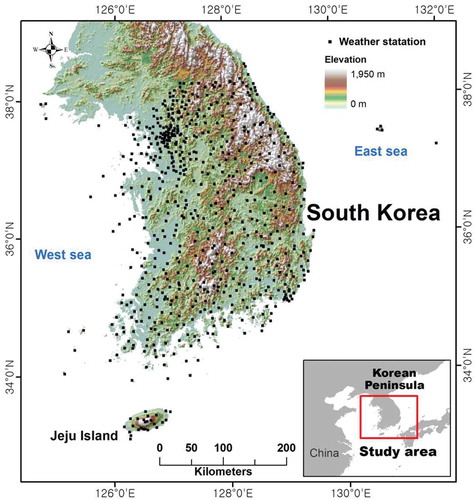
The study area was geographically located in the middle-latitude temperate climate zone with four distinct seasons. The winters are cold and dry because of the cold and dry continental high pressure; the summers are humid because of the hot and humid North Pacific high pressure. There are several clear, dry days in the spring and autumn because of migratory anticyclones.

Jeju Island, lying to the south of the study area, is a volcanic island with elevations ranging from 0 m to 1950 m above sea level. The distributions of precipitation, temperature, and wind vary according to the slope and elevation above sea level (Choi 2013). The location is optimal for analyzing spatial distribution of climate as 23 weather observation stations are available on this island (Park and Jang 2008).

Monthly wind speeds were obtained for the period March 2011-February 2014 at 529–641 stations across South Korea, including stations on small islands. The wind speeds observed on the small islands were used as input data as they are important for interpolating the coastal wind speeds on Jeju Island and mainland South Korea. Figure 2 depicts the distribution of the observation stations on February 2014. The density of the network was highest in June 2013, with 641 stations. The number of stations was lowest, at 529, in December 2011. Some observation stations were relocated during the research period. Hence, for this study, the available stations and their locations were verified monthly and utilized in the interpolation.

The range of measured wind speeds during the 2011-2014 period was 0.1–10.0 m/s, with the coastal areas and mountain tops indicating relatively high speeds. Spring (2.4 m/s) and winter (2.1 m/s) had the highest seasonal average wind speeds; summer (1.9 m/s) and autumn (1.9 m/s) had the lowest average. The wind direction of the study area was mainly northwesterly in the spring and winter and southwesterly in the summer. Winds were generally weak in September and October. There was a clear influence of land and sea breezes and strong winds in the coastal areas.

Weather stations are uniformly distributed within South Korea. The northwestern areas of South Korea and Seoul have the highest concentration of stations. The elevations of the stations range from approximately sea level (Suyu, the southwestern coastal region, 1 m) to above 1600 m (Witse-Oreum, Jeju Island, 1672 m). Approximately, 80% of the stations, however, are located below 200 m (Figure 3).

Figure 3. Cumulative percentage of stations from various elevations, February 2014.

2.3. Interpolation and evaluation methods

In this study, MK-PRISM and co-kriging interpolation methods were used. Tables 1 and 2 display the composition of the primary parameters and selected values of MK-PRISM and co-kriging, respectively. Parameter values are expressed as ranges in both tables because their values are used differently on a monthly basis.

Table 1. MK-PRISM parameters and ranges of optimized values by the SCE-UA.

Parameter	Description	Unit	Range
Main function
Radius	Search radius is used to collect nearby known stations	km	50
Weighting importance scalar (appendix Equation (A2)
Fd	Distance weighting importance scalar	–	0.5–0.6
Fz	Elevation weighting importance scalar	–	0.5–0.6
Distance weighting (appendix Equation (A3))
rm	Minimum radius of influence	km	1.0
a	Distance weighting exponent	–	0.88–0.96
Elevation weighting (appendix Equation (A4))
zm	Minimum elevation difference	m	100
zx	Maximum elevation difference	m	1000
b	Elevation weighting exponent	–	0.48–0.82
Coastal weighting (appendix Equation (A6))
v	Coastal proximity weighting exponent	–	0.88–0.95
px	Maximum coastal proximity difference	km	3
Parameter(wind speed)-elevation regression (appendix Equation (A7))
β1x	Default maximum slope for cell P/E regression function	m/s/m	0.004–0.007

In Table 1, r_m and p_x are fixed values that were determined through a trial and error process. z_m and z_x were determined based on previous studies (Daly et al. 2002, 2008; Kim et al. 2012). Radius is a variable used for determining the base point to be applied in the interpolation process. Weather stations are typically distributed at 15-20 km intervals in the study area. Hence, to ensure a sufficient inclusion of observation stations from the interpolating grid, the data search radius was set at 50 km. F_d, F_z, a, b, v, and β_1x were determined by parameter optimization and the ranges of the values are as indicated in Table 1. The sum of F_d and F_z is always equal to one. For example, if the F_d is 0.6, F_z will be 0.4.

The results of co-kriging were determined by the data search radius, type of kriging, and factors of the variogram. Among the different kriging types, ordinary kriging was used as the kriging type, as it deduces good interpolation results in the existing climate data interpolations such as precipitation and temperature (Park and Jang 2008; Park and Kim 2009).

Factors of the variogram are the model, relative distance, nugget, and sill value. In Table 2, the spherical model and relative distance were determined to be from 87 to 92 km by optimization. The sill value was determined considering the difference in wind speed and elevation that could appear within the maximum relative distance. The nugget range of the primary and secondary variables was also determined by parameter optimization. The nugget value in the cross-variogram, which indicates the correlation between the primary and secondary variables, was determined using Equation (1):

(1)

Table 2. Co-kriging parameters and ranges of optimized values by the SCE-UA.

	Parameter	Unit	Range
	Model	–	Spherical model
Relative distance		km	87–92
Primary variogram (wind speed)	Nugget1	m/s	0.2–0.5
	Sill	m/s	8.0–9.6
Secondary variogram (elevation)	Nugget2	m	166–267
	Sill	m	527–836
Cross variogram	Negget3	–	5–7.9
	Sill	–	1.1–1.6

where Nugget₃ is the nugget of the cross-variogram and Nugget₁ is the nugget of the primary variogram. Nugget₂ is the nugget of the secondary variogram. This setting is to satisfy the positive plus sign of the covariance matrix in the cross-variogram modeling.

The values of the parameters were determined using SCE-UA (Duan, Sorooshian, and Gupta 1992), which is a global optimization method. SCE-UA repeatedly estimates the parameter value within a given range of values until it converges with the objective function value. In this paper, KGE (Gupta et al. 2009) was used as the objective function value. KGE is given as:

(2)

where r is the Pearson product-moment correlation coefficient, α is the ratio between the standard deviation of the simulated values and the standard deviation of the observed values, and β is the ratio between the mean of the simulated values and the mean of the observed values.

Further, RMSE was used to compare the two model efficiencies with KGE. RMSE is given by the following equation:

(3)

where n is total number of samples, y_i is the observed values, and ŷ_i is the simulated values at time i.

KGE and RMSE were calculated using jackknife cross-validation (Yates and Warrick 1987). Jackknife cross-validation compares the observed and simulated values at a point with the input data while excluding one observation station at a time. This method is useful for evaluating model performance as it can reduce the uncertainty that may arise in the process of classifying the input data into the training and testing sets.

3. Results

3.1. Spatial distribution of measured wind speed

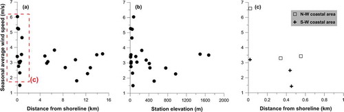
Coastal proximity has an important role in the distribution of wind speed and elevation. Spatial distribution of wind speed is strongly influenced by the distance from the shoreline, considerably more than other data such as precipitation or temperature. Seasonal average wind speed increases as elevation increases; however, it decreases as the distance from the coast increases. Figures 4 and 5 demonstrate the effects of terrain elevation and coastal proximity on the spatial distribution of wind speed. Figure 4 depicts wind speeds at the weather stations located between the south coast and Mount Jiri. Wind speed decreases as the distance from the coast increases up to 15-20 km from the coast (Figure 4(a)). Wind speed increases with elevation; however, this is difficult to confirm in regions below 200 m above sea level (Figure 4(b)). This is because of the effect of the coast, as indicated in Figure 4(a). Equation (4), which is the exponentiation of the coastal proximity and elevation, illustrates that wind speed also increases as coastal proximity and elevation increase (Figure 4(c)):

(4)

Figure 4. For the Spring season during the 2011–2014, March, April, and May, the average wind speed in (a) distance from shoreline; and (b) station elevation in Jiri Mountain.

Figure 5. For the Spring season during the 2011–2014, March, April, and May, the average wind speed in (a) distance from shoreline; and (b) station elevation in Jeju Island.

where w is the weight of the coastal proximity and elevation combined, d is the distance to a target station from the shoreline, and d_m is the distance to the farthest station from the shoreline. z is the elevation of a target station, z_m is the elevation of the highest station, and 0.3 and 0.7 are the weights for elevation and coastal proximity, respectively. The values were empirically determined.

The wind speed distribution at Jeju Island effectively depicts the above relationship. Figure 5(a) indicates that wind speed varies from approximately 1–7 m/s at distances within 2 km from the shoreline. Wind speed gradually decreases until 10 km, where the wind speed begins to increase again. Figure 5(b) illustrates that the reason the wind speed increases at this point, distant from the shoreline, is because of the increase in elevation. Therefore, the coastal effect is stronger to a certain point, after which the effect of elevation becomes stronger.

Figure 5(c) displays the wind speed at points along the same slope among the points located within 2 km of the coast (dotted box in Figure 5(a)). The wind speed at locations along the coast among points located in the north-west coastal area is approximately 7 m/s. The wind speed at points located 300–500 m from the shoreline is approximately 3 m/s. The wind speed at points along the coast among the points located in the south-west coastal area is 3 m/s. The wind speed at points 400–500 m from the shoreline ranges from 1 to 2.5 m/s.

The rate of decrease in wind speed according to distance from the coast observed in Figure 5(c) is greater than that observed in Figure 5(a). Whereas there is only approximately a 2 m/s decrease about 4–12 km in Figure 5(c), there is an approximately 3 m/s decrease (north-west coastal area) or approximately 1.5 m/s decrease (south-west coastal area) at 500 m. This signifies that the coastal effect is greater than other areas in points within 2 km from the coast.

Further, spatial distribution of the wind speed depends significantly on the type of land, for example, wind speed at a ridge may be higher than other landforms. Because the observation from the ridge is low, in the interpolation process, the gradient of the linear regression line between wind speed and elevation varies dramatically, especially when the observation point used. Figure 6 indicates the wind speed at the stations located in the west part of Mt. Deogyu. The wind speed is 3.8 m/s at the ridge of the mountain and the slope of the linear regression is 0.0023 when the known point is used in the interpolation process. The slope is 0.0011 when the known point is not used. Despite similar land surface, there is a significant difference in the wind speed pattern. Therefore, new methods to facilitate spatial consistency of wind speed are required to apply MK-PRISM for wind speed interpolation.

Figure 6. Relationship between monthly mean wind speed and elevation when a station (STN. 314) included (solid line) and excluded (dashed line) in February 2014.

3.2. Modification of MK-PRISM

The deficiency of the MK-PRISM method in wind speed interpolation is that it represents similar wind speed along shorelines and landforms including valleys, slopes, and ridges. The gradient of the linear regression line between wind speed and elevation is abruptly changed when some observation points are used (Park and Jang 2015). Therefore, two MK-PRISM algorithms were modified for application to wind speed interpolation.

In the MK-PRISM for precipitation and temperature, the precipitation of the target grid cell is determined based on the linear regression equation between precipitation and elevation. In the MK-PRISM for wind speed, however, it was modified to consider the linear regression equation between wind speed and costal proximity for wind speed within a certain distance from the coast (Figure 7). This is a similar concept to the use of two vertical layers in PRISM to consider the temperature inversion layer as in Daly et al. (2008) paper.

Figure 7. Difference between wind speed in near shoreline and wind speed in the other region in modified MK-PRISM.

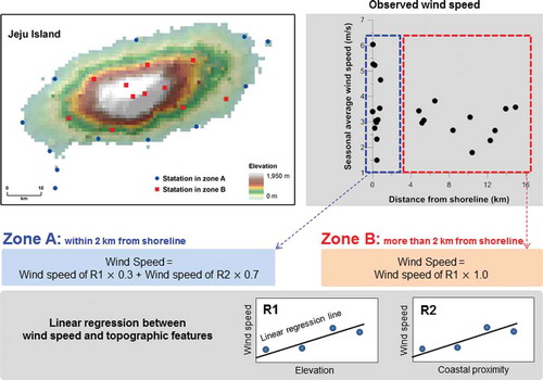
Based on an analysis of Figure 5, in the present study, the particular distance from the coast is set at 2 km. Both the wind speed determined based on the linear regression equation between wind speed and elevation and the wind speed based on the linear regression equation between wind speed and coastal proximity, have been evaluated at this distance. The final wind speed was determined by multiplying the two wind speeds with weights of 0.3 and 0.7, respectively. Wind speed greater than 2 km from the coast was estimated based on the linear regression equation between wind speed and elevation. In this case, coastal proximity is used as the weight in Equation (A2) in determining wind speed.

In the MK-PRISM for wind speed, coastal proximity affects wind speed in 2 km intervals from the coastline. The maximum effective distance of coastal proximity is 20 km from the coastline. This is because the effects of coastal proximity were found to weaken after approximately 15–20 km in Figure 4(a). Beyond this distance, the effect of coastal proximity in MK-PRISM dissipates and the effect of elevation is emphasized.

Further, a wind speed increase due to an elevation increase in Jeju Island (Figure 5) can be seen in the observation data of the two stations located higher than 1600 m above sea level. The names of these stations are Witse-Oreum (1673 m above sea level) and Jindallae-bat (1490 m above sea level). Wind speed data since 2011 were obtainable for these points. Although data from 2003–2010 were also available, they were deemed to contain errors that limited their usage (they have not been presented in this paper). As the elevation differences between stations are rather insignificant, other than these two data sets, confirming an increase in wind speed due to an increase in elevation is difficult. Hence, if the two data sets cannot be used because of outliers or lack of observations, the linear regression equation of elevation–wind speed could have a negative slope, resulting in the simulated wind speeds on mountain areas being less than the surrounding areas.

There is a possibility that this could occur more frequently in the mainland of South Korea because approximately 80% of the weather stations in South Korea are located below 200 m above sea level. Moreover, owing to coastal proximity effects, the elevation–wind speed relationship may not be appropriately simulated in areas near the coast.

Hence, if the linear regression equation of elevation–wind speed (β₁ of Equation (A7) displayed a negative slope, the slope was adjusted to a minimum positive value (β_1m of Equation (A7)). If the slope was overly steep, the value was adjusted to a maximum value (β_1x of Equation (A7)). According to Park and Jang (2015), this adjustment process is not effective in controlling a sudden change of the slope appearing in similar land surfaces. This study adjusted the slope using Equation (5) as Park and Jang (2015) suggested.

(5)

where β_1xn is the new maximum allowable value of β₁, β_1x is the default maximum value, and T is the classification of landform based on the Topographic Position Index (Weiss 2001). The monthly β_1x are determined as indicated in Table 1 through parameter optimization. β_1mn is the new minimum allowable value of β₁.

3.3. Comparison of model performance

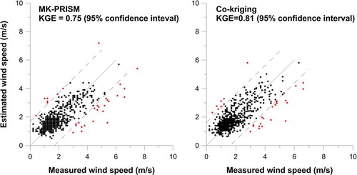
MK-PRISM and co-kriging did not demonstrate significant differences in monthly mean wind speed interpolation performance. Figure 8 illustrates the relationship between the predicted wind speed and measured wind speed for the monthly mean wind speed of February 2014, which was interpolated using MK-PRISM and co-kriging. Whereas both MK-PRISM and co-kriging significantly underestimated or overestimated a small number of points, the majority of the points generally converged and were distributed along the 1:1 ideal regression line. The KGE of MK-PRISM and co-kriging at the 95% confidence interval were 0.75 and 0.81, respectively.

Figure 8. The KGEs of the MK-PRISM and co-kriging in monthly mean wind speed at the February 2014. The line in the center denotes 1:1 ideal regression line. The outer, dash lines denote the 95% confidence interval for an individual estimated value.

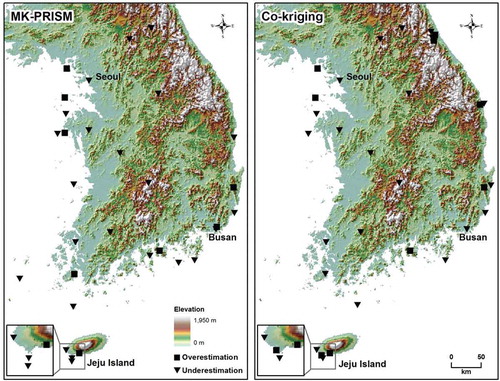
Figure 9 is the distribution of points outside the 95% confidence interval lines. Points where both MK-PRISM and co-kriging recorded significant estimation errors were mainly located in the coastal areas, islands, and mountain summits. In MK-PRISM, 23 of the 31 points were located in coastal or island areas, of which 16 were underestimated. In co-kriging, 18 of the 31 points were located in the aforementioned areas, of which 15 were underestimated. Inland, both methods generally produced underestimations; stations with significant errors were located on the mountain summits. Hence, both models tended to underestimate the high wind speed that appeared at specific mountain summits, coastal, and island observation stations.

Figure 9. Spatial distribution of points that are located outside of the 95% confidence interval lines in Figure 8.

Table 3 indicates the monthly mean KGE and RMSE of the two models at the 95% confidence interval. The average KGEs of MK-PRISM is 0.72; co-kriging is 0.75. The average RMSEs of MK-PRISM and co-kriging are 0.54 and 0.57 m/s, respectively.

Table 3. Model performances of the MK-PRISM and co-kriging in the 95% confidence interval.

Month	KGE		RMSE (m/s)
	MK-PRISM	Co-kriging	MK-PRISM	Co-kriging
January	0.74	0.77	0.61	0.65
February	0.73	0.77	0.60	0.61
March	0.69	0.74	0.61	0.64
April	0.70	0.74	0.58	0.61
May	0.70	0.73	0.48	0.51
June	0.68	0.74	0.44	0.46
July	0.72	0.73	0.53	0.55
August	0.72	0.76	0.48	0.50
September	0.73	0.76	0.46	0.49
October	0.75	0.78	0.49	0.52
November	0.73	0.76	0.59	0.62
December	0.74	0.77	0.66	0.68
Average	0.72	0.75	0.54	0.57

The minimum KGE of MK-PRISM was 0.68; the maximum was 0.75. The minimum and maximum KGE of co-kriging were 0.73 and 0.78, respectively. Both methods recorded the lowest KGE in the spring (March/April/May) and the highest in winter (December/January/February). This is because both models underestimated the value of certain stations when the highest wind speeds of the spring north-westerly seasonal wind were observed at island and coastal areas. RMSE was highest in winter (December/January/February) and spring (March/April/May) when wind speeds increase and lower in the summer (June/July/August) and autumn (September/October/November) when wind speeds decrease. Both MK-PRISM and co-kriging had an RMSE range of 0.44–0.68 m/s. The KGE of MK-PRISM and co-kriging generally had a difference of 0.03 and an RMSE difference of 0.03 m/s. In conclusion, there is no marked difference between the two models.

3.4. Comparison of wind speed maps

In the present study, monthly mean wind speed distribution maps were created for the period of March 2011–February 2014. Figure 10 depicts the monthly mean wind speed in terms of seasonal average wind speed.

Figure 10. Estimated seasonal average wind speed (2011–2014).

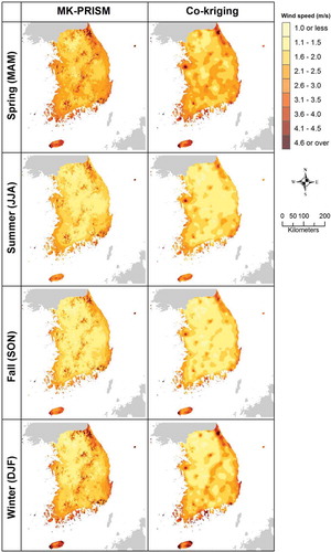
The results of MK-PRISM demonstrate that the distribution of wind speed is affected by elevation, coastal proximity, and topographic facet. The wind speed patterns are clear along the Taebaek Mountain range in Eastern South Korea. The average wind speed in the spring is high on the ridges of the eastern mountain area and the eastern aspect and low on the western aspect. High-speed winds appear along the western and southern coasts and the inland Sobaek Mountain range. Wind speeds are high on the coasts of Jeju Island and on Hanra Mountain. Wind speeds are relatively lower in the inland basins. The wind speed distribution pattern is clearest in the spring and winter.

The wind speed distribution of co-kriging was generally similar to MK-PRISM. The two, however, differed in the wind speed distribution pattern. For example, in the wind speed distribution for spring, MK-PRISM clearly differentiates the eastern aspect (the aspect closer to the East Sea) and the western aspect of the eastern mountain range. Co-kriging, conversely, does not clarify the effect of aspects on wind speed distribution. Moreover, the distribution of wind speed along the ridges of the inland mountain range is less clear than that of the MK-PRISM model.

The wind speed difference between the two models appears primarily on the eastern aspect of the eastern mountain range (Taebaek Mountain range). Other locations that indicate relatively significant differences in wind speed were the southern mountainous areas, parts of the west coast, and Jeju Island. Figure 11 illustrates the diversity in the spring season wind speed distribution of these four areas along with the respective terrain:

Figure 11. Estimated average wind speed during the spring 2011–2014.

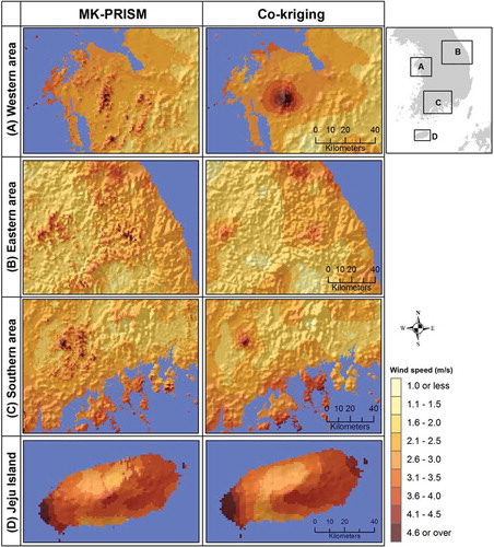
(A) In the western region, MK-PRISM effectively reproduced the high-speed winds that appear along the mountain summits, ridges, and coastlines, particularly the high-speed wind that appears near the coastline. Conversely, the high-speed winds observed in the mountain areas in co-kriging are dispersed widely among the surrounding areas. Whereas the wind speed in the coastal regions is higher than other areas, the distribution of wind speed that appears along the coastline is not well reproduced.

(B) MK-PRISM accurately reproduced the high-speed wind that appears along the ridges of the eastern region. Low-speed winds are presented in the basin area on the bottom of the figure. The wind speed distribution produced by co-kriging is generally similar to that of MK-PRISM, except that the wind speed along the ridges differs somewhat.

(C) MK-PRISM displayed relatively high-speed winds on the mountain summits, ridges, and inclines toward the coast in the southern area. Although co-kriging also displayed high-speed winds on the mountain summits and in the coastal areas, there was less continuity on the ridges.

(D) On Jeju Island, MK-PRISM effectively reproduced the high-speed winds that appear on the coasts and mountain summits, particularly the belt of high wind speeds that appear along the west-to-north, and north-to-east coasts. In co-kriging, there were no high-speed winds in the form of a belt along the coast and the vicinity of mountain summits indicated relatively low-speed winds. This may have been due to the low-speed winds observed at the middle mountainous area also affecting the mountain summit. The low-speed winds of the middle mountainous area had limited presence around the observation area and did not affect the mountain summit in MK-PRISM.

4. Discussion

In the quantitative comparison results, the KGE and RMSE of the models were similar and satisfactory. The KGE of MK-PRISM and co-kriging had 0.03 difference and the RMSE values of these two methods had 0.03 m/s difference. The distribution of points of significant error was also similar. These results demonstrate that the simulations of the MK-PRISM and co-kriging models were similar in the lowlands. This is because approximately 80% of the stations are located below 200 m and the efficiencies calculated using resampling data selected by the Jackknife method. Therefore, the simulation results of the two models do not differ significantly in the rolling lowlands where there are many available weather stations.

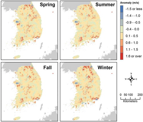
In the qualitative comparison results, the spatial distributions of wind speed were different. High-speed winds appeared continuously along the coastline and ridges in MK-PRISM. Co-kriging, conversely, did not indicate such distribution. Figure 12 displays that the difference between the two models in primarily mountainous areas. This indicates that the structural differences between the two models have a significant effect on the simulation results in areas that lack weather stations.

Figure 12. Anomaly of the estimated seasonal average wind speed between the MK-PRISM and co-kriging.

Co-kriging attempts to ensure the connectivity of the wind speed at similar elevations with observation points using a secondary variable; however, there is a limitation. For example, the result of co-kriging in Figure 11(c) illustrates the limitation clearly. A weather station located on the mountain summit is displayed in Figure 11(c). Wind speed is reduced as distance increases from the mountain summit and the result cannot reproduce the distribution of wind speed that can appear along the ridge. Although the elevation is used as a secondary variable, the effect of topography is not sufficiently represented.

The bias of the observation data also causes imperfection in co-kriging. The observation data are biased because observation points are relatively concentrated in the lowlands. This limitation of data is also found in the data of other countries, for example, the United States, England, and Wales (Daly, Neilson, and Phillips 1994; Luo, Taylor, and Parker 2008). Fortunately, observations are located on both lowlands and uplands in Jeju Island. Therefore, the positive relationship between elevation and wind speed was confirmed in Figure 5.

However, as mentioned in the text, confirming an increase in wind speed due to an increase in elevation is difficult in the majority of areas because of data bias. When there was no observation point in a mountain area, co-kriging was unable to reproduce the wind speed properly, even when the elevation was used as a secondary variable.

MK-PRISM did reproduce the relatively high wind speeds that appeared in the continuous terrain such as ridges and along the coastline. This model has three specifications: (1) MK-PRISM considers topographical similarity between target grid cell and known points with weightings of known points determined by topographical factors; (2) only a positive relationship is allowed for the slope of the linear regression line between wind speed and elevation; (3) MK-PRISM determines wind speed by strongly reflecting the effect of coastal proximity up to 2 km inland from the coast. These specifications have significant effects on the results.

Additional verification may be required to determine what model is more appropriate to represent the reality in mountainous and coastal areas. In general, wind speed increases with elevation and proximity to the coast (Luo, Taylor, and Parker 2008; Philippopoulos and Deligiorgi 2012; Robert, Foresti, and Kanevski 2013). We also know that similar wind speeds appear continuously along ridges or coastlines. Hence, the wind speed distribution presented by MK-PRISM appears to be more realistic.

The results of this study verify that the benefits of MK-PRISM are derived from the flexibility of the material and algorithms. MK-PRISM can outperform co-kriging in estimating the spatial distribution of wind speed. Furthermore, as MK-PRISM can create more combinations of topographic features than co-kriging, it has a greater chance of being practical for wind speed interpolation. This capability of MK-PRISM has significant potential for geographical information system (GIS) and remote sensing using geostatistical analysis because MK-PRISM can be an approach to reveal the spatial distribution of mineral resources (Jaber, Ibrahim, and Al-Muhtaseb 2013), soil organic carbon (Simbahan et al. 2006; Wang, Zhang, and Li 2012), groundwater (Goovaerts et al. 2005), forest biomass (Sales et al. 2007), morphological factor (Tang 2005), and sediment quality (Yan et al. 2014). However, it requires gridded data such as a satellite image that correlates with observation point data. Prior to the use MK-PRISM, it was necessary to correlate the data to be certified.

The characteristic errors that appeared in simulation results have illustrated that observation data of some stations require addressing outliers. The errors of the two models frequently appeared at observation stations located on distinctive topography. For example, the highest wind speed (6.6 m/s) and highest prediction error (2.74 m/s) in Figure 9 appear at the Gosan Station. Because this station is located on top of the western coastal cliffs of Jeju Island, strong westerly gales can be present. Conversely, other weather stations are located on the low plains, leading to lower wind speeds than the Gosan Station. Similar to the Gosan Station, the wind speeds observed on the coast are from 3.7 to 3.8 m/s, as the coastal stations are located on low plains. It is therefore difficult to predict the wind speed at the Gosan Station using the wind speed from nearby stations.

This means that the Gosan Station is not located at a point that represents the wind speed of the peripheral region. The wind speeds on Western Jeju Island in interpolation results appear to be overestimated because of the wind speed at Gosan Station (Figure 11(d)). Therefore, the wind speed at Gosan Station could be considered as an outlier in a further study.

From another perspective, island areas, including Jeju Island, may require estimation of wind speed using a model structure or parameter value different from that of the inland areas. This is because points with high estimation errors appeared mainly in island areas and the effect of coastal proximity is somewhat different in Figure 4 (south coast Jiri Mountain) and Figure 5 (Jeju Island). This will require further research.

5. Conclusions

In the present study, an MK-PRISM model was developed for wind speed interpolation. In MK-PRISM, the weighting of coastal proximity has been measured from the shoreline and continues to 20 km (2-km intervals). The measured wind speed indicated that the distance from 0 to 20 km from shoreline is an effective distance in wind speed estimation. The effect of coastal proximity is particularly emphasized in areas within 2 km from the shoreline. Further, this study controlled the allowable range of the slope of the linear regression equation based on landform classification to prevent sharp changes in wind speed distribution, despite continuous similar topography.

The quantitative evaluation based on model performances and qualitative evaluation based on wind speed maps confirmed that MK-PRISM is useful for wind speed interpolation. The distinct characteristic of MK-PRISM compared to co-kriging was that it effectively reproduced the high-speed winds that appear along the coastline and ridges, and the homogeneous low-speed wind areas of the basins in mainland South Korea.

The present study contributes to understanding the relationship between wind speed and topography by applying wind speed to MK-PRISM. The results verified that the topographic features (e.g., terrain convexity, aspect, coastal proximity) considered in MK-PRISM were important factors that control the spatial distribution of wind speed. A model based on such understanding of the relationship between factors can generate a more realistic wind speed spatial distribution than a model that simply uses the relationship between elevation and wind speed.

MK-PRISM had difficulty in reproducing the extreme high-speed winds that appear on some coasts, islands, and mountain summits in the cross-validation process. This can be resolved through future research such as model improvement, parameter differentiation according to region, and outlier management in the input data.

This finding is meaningful because it may lead to the spatial interpolation of different GIS and remote sensing data correlated with topographical features, especially in a shortage of observation data. Furthermore, the wind speed distribution map generated by MK-PRISM is practical for other geographic studies.

Acknowledgment

This work was supported by the research grant of the Kongju National University in 2014.

Disclosure statement

No potential conflict of interest was reported by the authors.

Additional information

Funding

This work was supported by the Kongju National University.

Appendix 1. MK-PRISM

MK-PRISM is a modified version of PRISM. PRISM creates a primary linear regression line between the climate value measured at the observation stations and the elevation after assigning weights to the stations used in interpolation. The climate value of the last station is estimated based on the regression line. The weight of each station is determined by the following Equation (A1):

(A1)

where W is the combined weight of a station, W_c, W_d, W_z, W_p, W_f, W_l, W_t, and W_e are the cluster, distance, elevation, coastal proximity, topographic facet, vertical layer, topographic position, and effective terrain weights, respectively, and F_d and F_z are user-specified distance and elevation weighting importance scalars (Daly et al. 2008). In MK-PRISM, the equation above is simplified (Kim et al. 2012), as in Equation (A2).

(A2)

Distance weighting is calculated by Equation (A3). Because the climate similarity between two stations generally decreases as the distance increases, the distance weighting is calculated using a formula that is inversely proportional to the square of the distance:

(A3)

where d is the lateral distance between a target cell and a known point. The calculation is conducted only for observation points located within the r radius of influence, which is the distance between the grid point and the observation point.

The topography elevation weighting is calculated by Equation (A4):

(A4)

where ∆z is the difference in elevation between a target cell and a known point. The similarity between two climates decreases as the difference in elevation increases. If the elevation difference is greater than ∆z_x, it is considered not similar. The quantities ∆z_m and ∆z_x are the minimum elevation difference and maximum elevation difference, respectively.

The topographic facet weight is calculated by Equation (A5):

(A5)

where ∆f is the difference in aspect between a target cell and a known point, B is the number of obstacles (contradicting aspects) between the two, and c is the facet weighting exponent. The appropriate value of c depends on the importance of topographic facets in the modeling region (Daly et al. 2002).

The coastal proximity weight is calculated by Equation (A6):

(A6)

where ∆p is the difference in coastal proximity between a target cell and a known point. The weight decreases as the coastal proximity difference between two points increases, as there is a greater chance of the climates being different. p_x is the maximum coastal proximity difference, above which proximity weight is zero. v is the coastal proximity weighting exponent.

After the weight is determined for each known point, the value of the target grid cell is calculated by Equation (A7):

(A7)

where Y is the predicted climate element, β₁ and β₀ are the regression slope and intercept, respectively, X is the digital elevation model (DEM) elevation at the target grid cell, β_1 m and β_1x are the minimum and maximum allowable regression slopes, w_i is a weighting value, and x_i and y_i are elevation and climate values, respectively.

Detailed explanations of PRISM and MK-PRISM can be found in Daly et al. (2008) and Kim et al. (2012), respectively.

Appendix 2. Co-kriging

Co-kriging is a method that involves interpolation by linear summation of two or more variables. In co-kriging, the primary variable is the variable to be estimated; variables other than the primary variable are called secondary variables. Co-kriging performs interpolation by composing a variogram between the primary variable and secondary variables after composing a variogram for each of the primary and secondary variables. The general formula of co-kriging is:

(B1)

where z is the primary variable, n is the total number of data used for the primary variable, n_s is the total number of secondary variables used, u_j is the jth secondary variable, m_j is the total number of data for the jth secondary variable, λ is the weight, and x is the location of each datum. The total number of variables (n_s + 1) and number of data (n + n_s × m_j) are used to estimate the value of the primary variable.

Co-kriging additionally utilizes the distribution of information of the secondary variables when there are a minimal number of primary variables and many correlated secondary variables. Because the spatial distribution of wind speed is correlated to elevation (Luo, Taylor, and Parker 2008), elevation has been used as a secondary variable in this paper.

References

- Archer, C. L., and M. Z. Jacobson. 2013. “Geographical and Seasonal Variability of the Global “Practical” Wind Resources.” Applied Geography 45: 119–130. doi:10.1016/j.apgeog.2013.07.006.
- Beier, C. M., S. A. Signell, A. Luttman, and A. T. DeGaetano. 2011. “High-Resolution Climate Change Mapping with Gridded Historical Climate Products.” Landscape Ecology 27 (3): 327–342. doi:10.1007/s10980-011-9698-8.
- Cellura, M., G. Cirrincione, A. Marvuglia, and A. Miraoui. 2008. “Wind Speed Spatial Estimation for Energy Planning in Slicily: Introduction and Statistical Analysis.” Renewable Energy 33 (6): 1237–1250. doi:10.1016/j.renene.2007.08.012.
- Choi, G. 2013. “Spatial Patterns of Seasonal Extreme Precipitation Events in Mt. Halla.” Journal of Climate Research 8 (4): 267–280. doi:10.14383/cri.2013.8.4.267.
- Choi, J., W. H. Cooke, and M. D. Stevens. 2009. “Development of a Water Budget Management System for Fire Potential Mapping.” GIScience & Remote Sensing 46 (1): 39–53. doi:10.2747/1548-1603.46.1.39.
- Cooke, W. H., G. V. Mostovoy, V. G. Anantharaj, and W. M. Jolly. 2012. “Wildfire Potential Mapping over the State of Mississippi: A Land Surface Modeling Approach.” GIScience & Remote Sensing 49 (4): 429–509. doi:10.2747/1548-1603.49.4.492.
- Daly, C., W. P. Gibson, G. H. Taylor, G. L. Johnson, and P. Pasteris. 2002. “A Knowledge-Based Approach to the Statistical Mapping of Climate.” Climate Research 22 (2): 99–113. doi:10.3354/cr022099.
- Daly, C., M. Halbleib, J. I. Smith, W. P. Gibson, M. K. Doggett, G. H. Taylor, J. Curtis, and P. P. Pasteris. 2008. “Physiographically Sensitive Mapping of Climatological Temperature and Precipitation across the Conterminous United States.” International Journal of Climatology 28 (15): 2031–2064. doi:10.1002/joc.1688.
- Daly, C., R. P. Neilson, and D. L. Phillips. 1994. “A statistical-Topographic Model for Mapping Climatological Precipitation over Mountainous Terrain.” Journal of Applied Meteorology 33 (2): 140–158. doi:10.1175/1520-0450(1994)033<0140:ASTMFM>2.0.CO;2.
- Duan, Q., S. Sorooshian, and V. K. Gupta. 1992. “Effective and Efficient Global Optimization for Conceptual Rainfall-Runoff Models.” Water Resource Research 28 (4): 1015–1031. doi:10.1029/91WR02985.
- Fadare, D. A. 2010. “The Application of Artificial Neural Networks to Mapping of Wind Speed Profile for Energy Application in Nigeria.” Applied Energy 87: 934–942. doi:10.1016/j.apenergy.2009.09.005.
- Goovaerts, P., G. AvRuskin, J. Meliker, M. Slotnick, G. Jacquez, and J. Nriagu. 2005. “Geostatistical Modeling of the Spatial Variability of Arsenic in Groundwater of Southeast Michigan.” Water Resources Research 41 (7): W07013. doi:10.1029/2004WR003705.
- Gupta, H. V., H. Kling, K. K. Yilmaz, and G. F. Martinez. 2009. “Decomposition of the Mean Squared Error and NSE Performance Criteria: Implications for Improving Hydrological Modelling.” Journal of Hydrology 377 (1–2): 80–91. doi:10.1016/j.jhydrol.2009.08.003.
- Hill, D. J. 2013. “An Assessment of Spatial Models for Daily Minimum and Maximum Air Temperature.” GIScience & Remote Sensing 50 (3): 281–300. doi:10.1080/15481603.2013.808459.
- Jaber, S. M., K. M. Ibrahim, and M. Al-Muhtaseb. 2013. “Comparative Evaluation of the Most Common Kriging Techniques for Measuring Mineral Resources Using Geographic Information Systems.” GIScience & Remote Sensing 50 (1): 93–111. doi:10.1080/15481603.2013.778550.
- Jiménez, P. A., J. F. González-rouco, E. García-bustamante, J. Navarro, J. P. Montávez, J. Vilá-Guerau De Arellano, J. Dudhia, and A. Muňoz-rolda. 2010. “Surface Wind Regionalization over Complex Terrain: Evaluation and Analysis of a High-Resolution WRF Simulation.” Journal of Applied Meteorology and Climatology 49: 268–287. doi:10.1175/2009JAMC2175.1.
- Kang, H. S., D. H. Cha, and D. K. Lee. 2005. “Evaluation of the Mesoscale Model/Land Surface Model (MM5=LSM) Coupled Model for East Asian Summer Monsoon Simulations.” Journal of Geophysical Research Atmospheres 110. doi:10.1029/2004JD005266.
- Kim, G. H., J. H. Youn, and B. S. Kim. 2010. “Producing Wind Speed Maps Using Gangwon Weather Data.” Journal of Korea Spatial Information Society 18 (1): 31–39. doi:10.9708/jksci.2010.15.8.031.
- Kim, M. K., M. S. Han, D. H. Jang, S. G. Baek, W. S. Lee, Y. H. Kim, and S. Kim. 2012. “Production Technique of Observation Grid Data of 1km Resolution.” Journal of Climate Research 7 (1): 55–68.
- Luo, W., M. C. Taylor, and S. R. Parker. 2008. “A Comparison of Spatial Interpolation Methods to Estimate Continuous Wind Speed Surfaces Using Irregularly Distributed Data Form England and Wales.” International Journal of Climatology 28: 947–959. doi:10.1002/joc.1583.
- Park, J., and D. H. Jang. 2015. “Development and Validation of MK-PRISM-Wind for Wind Speed Interpolation.” Journal of Climate Research 10 (4): 313–327. doi:10.14383/cri.2015.10.4.313.
- Park, J. C. 2009. “A Study on the Application of the National GIS and Environmental Observation Data for Assessment of Regional Water Balance: A Case of the Catchment of Guryang Stream.” Journal of the Korean Geographical Society 44 (4): 557–576.
- Park, J. C., and M. K. Kim. 2009. “A Study on the Use of a Terrain Aspect Variable in Producing the Precipitation Distribution Map applying Cokriging: A Case of Jeju Island.” Journal of the Korean Geomorphological Association 16 (3): 59–66.
- Park, J. C., and M. K. Kim. 2013. “Comparison of Precipitation Distributions in Precipitation Data Sets Representing 1 km Spatial Resolution over South Korea Produced by PRISM, IDW, and Cokriging.” Journal of the Korean Association of Geographic Information Studies 16 (3): 147–163. doi:10.11108/kagis.2013.16.3.147.
- Park, N. W., and D. H. Jang. 2008. “Mapping of Temperature and Rainfall Using DEM and Multivariate Kriging.” Journal of the Korea Geographical Society 43 (6): 1002–1015.
- Philippopoulos, K., and D. Deligiorgi. 2012. “Application of Artificial Neural Networks for the Spatial Estimation of Wind Speed in a Coastal Region with Complex.” Renewable Energy 38: 75–82. doi:10.1016/j.renene.2011.07.007.
- Phillips, D. L., and D. G. Marks. 1996. “Spatial Uncertainty Analysis: Propagation of Interpolation Errors in Spatially Distributed Models.” Ecological Modelling 91 (1–3): 213–229. doi:10.1016/0304-3800(95)00191-3.
- Pianalto, F. S., and S. R. Yool. 2013. “Monitoring Fugitive Dust Emission Sources Arising from Construction: A Remote-Sensing Approach.” GIScience & Remote Sensing 50 (3): 251–270. doi:10.1080/15481603.2013.808517.
- Reynolds, R. W., T. M. Smith, C. Liu, D. B. Chelton, K. S. Casey, and M. G. Schlax. 2007. “Daily High-Resolution-Blended Analyses for Sea Surface Temperature.” Journal of Climate 20 (22): 5473–5496. doi:10.1175/2007JCLI1824.1.
- Rhee, J., S. Park, and Z. Lu. 2014. “Relationship between Land Cover Patterns and Surface Temperature in Urban Areas.” GIScience & Remote Sensing 51 (5): 521–536. doi:10.1080/15481603.2014.964455.
- Robert, S., L. Foresti, and M. Kanevski. 2013. “Spatial Prediction of Monthly Wind Speeds in Complex Terrain with Adaptive General Regression Neural Networks.” International Journal of Climatology 33 (7): 1793–1804. doi:10.1002/joc.3550.
- Sales, M. H., C. M. Souza Jr., P. C. Kyriakidis, D. A. Roberts, and E. Vidal. 2007. “Improving Spatial Distribution Estimation of Forest Biomass with Geostatistics: A Case Study for Rondonia, Brazil.” Ecological Modelling 205 (1–2): 221–230. doi:10.1016/j.ecolmodel.2007.02.033.
- Shin, S. C., M. K. Kim, M. S. Suh, D. K. Pha, D. H. Jang, C. S. Kim, W. S. Lee, and Y. H. Kim. 2008. “Estimation on High Resolution Gridded Precipitation Using GIS and PRISM.” Atmosphere 18 (1): 71–81.
- Simbahan, G. C., A. Dobermann, P. Goovaerts, J. Ping, and M. L. Haddix. 2006. “Fine-Resolution Mapping of Soil Organic Carbon Based on Multivariate Secondary Data.” Geoderma 132 (3–4): 471–489. doi:10.1016/j.geoderma.2005.07.001.
- Simpson, J. J., G. L. Hufford, C. Daly, J. S. Berg, and M. D. Fleming. 2005. “Comparing Maps of Mean Monthly Surface Temperature and Precipitation for Alaska and Adjacent Areas of Canada Produced by Two Different Methods.” Arctic 58 (2): 137–161. doi:10.14430/arctic407.
- Skamarock, W. C., J. B. Klemp, J. Dudhia, D. O. Gill, D. M. Barker, W. Wang, and J. G. Powers. 2005. A Description of the Advanced Research WRF Version 2. NCAR Tech. Note. NCAR/TN 468+STR, 100. Boulder, CO: National Center for Atmospheric Research.
- Tang, T. 2005. “Spatial Statistic Interpolation of Morphological Factors for Terrain Development.” GIScience & Remote Sensing 42 (2): 131–143. doi:10.2747/1548-1603.42.2.131.
- Wang, K., C. Zhang, and W. Li. 2012. “Comparison of Geographically Weighted Regression and Regression Kriging for Estimating the Spatial Distribution of Soil Organic Matter.” GIScience & Remote Sensing 49 (6): 915–932. doi:10.2747/1548-1603.49.6.915.
- Weiss, A. D. 2001. “Topographic Position and Landforms Analysis.” http://www.jennessent.com/downloads/tpi-poster-tnc_18x22.pdf.
- Yan, Y., R. T. James, F. Miralles-Wilhelm, and W. Tang. 2014. “Geographically Weighted Spatial Modelling of Sediment Quality in Lake Okeechobee, Florida.” GIScience & Remote Sensing 51 (4): 366–389. doi:10.1080/15481603.2014.929258.
- Yates, S. R., and A. W. Warrick. 1987. “Estimating Soil Water Content Using Cokriging.” Soil Science Society of America Journal 51 (1): 23–30. doi:10.2136/sssaj1987.03615995005100010005x.