CryoSheds: a GIS modeling framework for delineating land-ice watersheds for the Greenland Ice Sheet

Abstract

Choice of watershed delineation technique is an important source of uncertainty for cryo-hydrologic studies of the Greenland Ice Sheet (GrIS), with different methods yielding different watersheds for a common pour point. First, this paper explores this uncertainty for the Akuliarusiarsuup Kuua River Northern Tributary, Western Greenland. Next, a standardized, semi-automated modeling framework for generating land-ice watersheds for GrIS land-terminating ice (henceforth referred to as CryoSheds) using geographic information systems (GIS) hydrologic modeling tools is presented. The framework uses ArcGIS and the ArcPy geoprocessing library to delineate two types of land-ice watersheds, namely those defined by: (1) a hydraulic pressure potential with varying water to ice overburden pressure ratios (k-value), which determines theoretical flow paths from the hydrostatic equation, using surface and bedrock digital elevation models (DEMs) and (2) a surface topography DEM alone. Lastly, a demonstration of the CryoSheds method is presented for seven remotely sensed proglacial pour points along the Aussivigssuit River (AR), Western Greenland, and its largest tributaries. GrIS meltwater runoff from these seven nested land-ice watersheds is estimated using Modele Atmospherique Regional (MAR) v.3.2 and runoff uncertainties due to watershed delineation parameter selection is estimated.

Keywords:

• Greenland Ice Sheet
• meltwater runoff
• geographic information systems
• hydrologic watershed modeling
• catchment boundary delineation

1. Introduction

Extracting hydrologic information from digital elevation models (DEMs) using geographic information systems (GIS)-based tools is common in terrestrial surface water systems where basic hydraulics dictate that water flows through preferential routes from areas of high to low elevation, both over the surface and through porous media. In such systems, GIS tools and DEMs are useful for simulating topographically defined flow routes and separating contributing hydrologic areas according to bounding watershed divides (Marks, Dozier, and Frew 1983; Moore et al. 1983; O’Callaghan and Mark 1984; Band 1986; Band et al. 2000). Recent advances in DEM generation technologies and techniques (e.g. Morlighem et al. 2011; Bamber et al. 2013; Morlighem et al. 2014; Noh and Howat 2015) have enabled similar GIS-based hydrologic routing (e.g. Yang et al. 2015, 2016) and watershed delineations for the Greenland Ice Sheet (GrIS) (e.g. Lewis and Smith 2009; Mernild, Liston, and van den Broeke 2012; Banwell, Willis, and Arnold 2013; Rennermalm et al. 2013; Smith et al. 2015; Lindbäck et al. 2015).

However, hydrologic processes in cryosphere systems differ from terrestrial systems. For ice sheets, principles of physics and hydraulics dictate that meltwater drains from areas of high to low pressure, the pattern of which is influenced by both bedrock and surface topography (Shreve 1972; Cuffey and Paterson 2010). Yet, a number of studies delineate watershed divides using surface topography alone, a direct analog for traditional terrestrial watershed delineation (e.g. Mernild and Hasholt 2009; Mernild et al. 2010; Bartholomew et al. 2011; Mernild et al. 2011; Palmer et al. 2011; Mernild, Liston, and van den Broeke 2012; Mernild and Liston 2012; Chandler et al. 2013; Cowton et al. 2013; Hasholt et al. 2013; Mikkelsen et al. 2013; Fitzpatrick et al. 2014; Hasholt, Khan, and Mikkelsen 2014; Yde et al. 2014). The hydraulic pressure potential and the surface DEM methods seek to represent different physical processes. The former uses pressure head differentials to account for subglacial runoff and routing, while surface DEM watersheds account solely for surface runoff and routing.

Watershed delineation techniques for ice sheets are further complicated by varying subglacial water pressures (e.g. Banwell, Willis, and Arnold 2013; Lindbäck et al. 2015), coarse DEM resolution, large DEM errors (especially bedrock DEM errors, see Figures S1–S4), and complex glacier geometry, which result in standard GIS toolboxes producing a number of small subbasins (primarily along the GrIS perimeter) that do not appear to be hydrologically accurate. Such uncertainties underscore the need for a standard and repeatable watershed delineation method for the GrIS. This is particularly relevant for: (1) glacial erosion estimates that are normalized by catchment area (e.g. Cowton et al. 2012); (2) runoff model calibration, validation, and comparison with field-measured proglacial river discharge (e.g. Smith et al. 2015; Lindbäck et al. 2015; Overeem et al. 2015); and (3) ocean transport studies that require accurate freshwater input volume and location information (e.g. Luo et al. 2016). The importance of this work is underscored by trends of increasing meltwater runoff (Hanna et al. 2005) and acceleration of the contribution from the GrIS to global sea level rise (Rignot et al. 2011).

The objective of this study is to offer a standardized approach for cryo-hydrologic watershed delineation of land-terminating outlet glaciers in Greenland. To achieve this, we begin by demonstrating the importance of a standardized approach by comparing glacier-surface runoff simulated by the Modèle Atmosphérique Régional (MAR) v.3.2 climate model (Tedesco, Fettweis, and Alexander 2013) with observed proglacial river outflow from 2008–2013 (Rennermalm et al. 2014) for the land-ice watershed of the Akuliarusiarsuup Kuua River Northern Tributary (AKN) (Figure 1), Western Greenland. Next, we present the CryoSheds modeling framework, which builds upon the recommendations of Smith et al. (2015) to use a multi-watershed approach by incorporating the hydraulic potential and surface DEM methods into a single modeling framework, and Banwell, Willis, and Arnold (2013) and Lindbäck et al. (2015) who propose watershed delineations that account for variations in subglacial water pressure. CryoSheds produces land-ice watersheds tributary to a defined proglacial pour point and differs from previous methods by coupling the ice sheet and proglacial zones and allowing flexible, user-defined proglacial pour points to be located anywhere between the ice edge and coastline. Finally, a feasibility demonstration of CryoSheds is shown for seven remotely sensed proglacial pour points along the Aussivigssuit River (AR), Western Greenland, and its largest tributaries (Figure 3).

Figure 1. The importance of watershed delineation method and technique is illustrated (A) for the Akuliarusiarsuup Kuua River, Northern Tributary (AKN) in Western Greenland where a long-term river gauging station (grey triangle) monitored river discharge and runoff from the Greenland Ice Sheet from 2008 to 2013 (Rennermalm et al. 2014). Only the area of the land-ice watershed below ~1600 m ice surface elevation is shown. The total observed river discharge for June, July, and August (JJA) 2008–2013 is plotted against the total MAR v.3.2 (Tedesco, Fettweis, and Alexander 2013) simulated runoff for hydraulic potential (B) and surface DEM (C) land-ice watersheds for the same time period. The dashed line notes locations where modeled and observed runoff would be equal. (D) Plots the total field measured river discharge with the total MAR runoff for JJA in each year (see Table S1 for summary of data used).

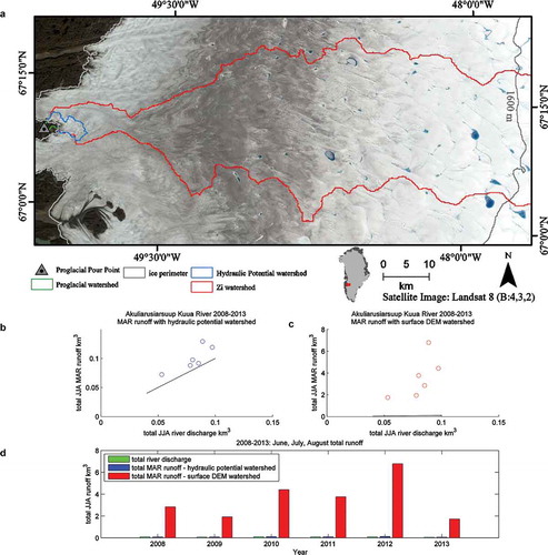
Figure 2. The final product of CryoSheds is a coupled land-ice watershed (red dashed line) that routes meltwater generated from the Greenland Ice Sheet to a proglacial pour point (triangle). To achieve this, ice subbasins (dashed grey lines) that contribute to the proglacial pour point are merged according to the modeled pour point (black circle) location and flow direction.

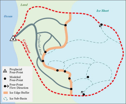
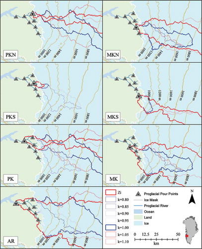
Figure 3. Map of CryoSheds land-ice watersheds for the seven proglacial pour points along the Aussivigssuit River (AR) and its major tributaries. Triangles denote proglacial pour point locations. Orange lines denote ice surface elevation contours.

2. A multi-watershed runoff comparison for the Akuliarusiarsuup Kuua River northern tributary

2.1 Study site, data, and methods

AKN is a tributary of the Watson River, which flows through Kangerlussuaq, Western Greenland. AKN remains frozen for most of the winter, yet after spring snowmelt and associated runoff from non-glaciated proglacial areas (3.62 km² of the land-ice watershed) AKN is primarily sourced by runoff from the GrIS. A long-term river discharge gauging station is located at a bridge crossing AKN ~2 km from the ice edge (Figure 1). River discharge data from this station is available at 30-minute intervals for the 2008–2013 melt seasons (Rennermalm et al. 2014). These data can be accessed on the PANGAEA Data Publisher for Earth and Environmental Science, at: https://doi.pangaea.de/10.1594/PANGAEA.838812. For this demonstration only the available data during June, July, and August (JJA), when melt is expected to be at its annual maximum, is used (summary of exact date ranges used for each year is included in Table S1).

The land-ice watershed for AKN is delineated using both hydraulic potential and surface DEM approaches (Figure 1). These approaches require (1) surface and basal DEMs; (2) a land/ice mask; and (3) a user-defined proglacial pour point (i.e. a point along a hydrologic network through which all runoff from a contributing watershed drains). For this demonstration, these datasets consist of: the IceBridge BedMachine Greenland version 2 surface DEM (spatial resolution 150 m) (Morlighem et al. 2015), which is derived from the Greenland Mapping Project (GIMP) Greenland surface DEM (Howat, Negrete, and Smith 2014); the BedMachine Greenland version 2 mass conservation bedrock DEM (Morlighem et al. 2011, 2014, 2015); the IceBridge BedMachine version 2 land cover mask, which is derived from the GIMP land-ice mask (Morlighem et al. 2015; Howat, Negrete, and Smith 2014); and the pour point location of the AKN gauging station. Land-ice watersheds are delineated following the CryoSheds modeling framework (see Section 3) assuming constant subglacial and ice overburden pressures (i.e. k = 1.00 as is assumed in Shreve 1972; Cuffey and Paterson 2010).

The gridded surface and bedrock DEMs are hosted by the National Snow and Ice Data Center (NSIDC) and are available in netcdf format at 150 m × 150 m posting in the Polar Stereographic North ESPG 3413 projection (Morlighem et al. 2015). The bedrock DEM uses a combined mass conservation and spatial interpolation approach that derives ice thickness from ice velocity calculated by satellite radar data collected between 2008 and 2009, and airborne radar surveys of ice thickness collected between 1993 and 2014 (Morlighem et al. 2011, 2014). Posted bedrock DEM errors for the GrIS range from 0 to 3490 m (Figures S1–S2). However, within the Western Greenland study area bed DEM errors range from 10 to 815 m and tend to be smaller at lower ice surface elevations within the ablation zone close to the ice edge (Figures S3–S4). The land/ice mask is bundled with the BedMachine data but is a downscaled version of the GIMP ice cover mask which classifies all of Greenland as grounded ice, floating ice, or ice-free land. This mask is created using the panchromatic band from Landsat 7 satellite imagery collected during July–September 1999–2001 and RADARSAT-1 Synthetic Aperture Radar amplitude images collected in fall 2000 (Howat, Negrete, and Smith 2014).

The total JJA runoff as measured at the AKN bridge between 2008 and 2013 is compared with total (JJA) modeled meltwater runoff from MAR v3.2 (see Table S1 for summary of exact date ranges used). MAR v3.2 uses European Center for Medium-Range Weather Forecasts (ECMWF) forcing data, a surface DEM, and an ice mask (Bamber et al. 2013) to calculate daily total runoff by solving energy balance equations for 25 km × 25 km grid cells spanning all of Greenland for the period 1958–2013 (Tedesco, Fettweis, and Alexander 2013). Runoff from grid cells intersecting AKN land-ice watersheds is summed to produce a total daily runoff estimate. For cells partially contained within AKN land-ice watersheds, the runoff contribution is weighted by the percent of each cell contained within the watershed.

To minimize bias in comparison with field data, the AKN gauge data are converted to a daily average runoff and then total daily discharge. Rennermalm et al. (2013) use the same AKN river discharge for 2008–2010 and find evidence of meltwater retention, storage, and wintertime release in the contributing ice watershed. This retention may explain some of the observed difference between river discharge and MAR runoff. However, for the purposes of this paper, we use only JJA data – collected during the active melt season. Additionally, to minimize the effects of lag time and hydrologic routing, we compare total river discharge with total MAR runoff. It is important to note that Rennermalm et al. (2013) also use a multi-watershed approach to suggest a range of possible watersheds. However, they use different input DEMs, thus it is difficult to discern if differences in results are a product of watershed delineation method or DEM source.

2.2 Land-ice watershed runoff comparison and the need for a standardized, multi-watershed approach

The land-ice watershed for AKN is 28.42 km² when derived using the hydraulic potential method, compared with 8772.5 km² when derived using the surface DEM approach. 74% of the surface DEM land-ice watershed lies above 1600 m, the approximate equilibrium-line altitude (ELA, Box and Bromwich 2004), while 0% of the hydraulic potential watershed falls above the ELA. The proglacial component of the AKN land-ice watershed is 3.62 km².

The JJA daily average discharge in the AKN river between 2008 and 2013 ranged from 3.68 to 19.22 m³ s⁻¹ with an overall average of 10.92 m³ s⁻¹ (Figure S6). The total JJA discharge ranged from 0.05 km³ in 2013 to 0.10 km³ in 2010. Total JJA MAR runoff summed across the hydraulic potential land-ice watershed ranges from 0.07 km³ in 2013 to 0.13 km³ in 2012. Total JJA MAR runoff for the surface DEM land-ice watershed ranges from 1.73 km³ in 2013 to 6.79 km³ in 2012 (Figure 1).

The significant differences between modeled runoff for the two watershed delineation methods given the same input DEMs, particularly in contrast to the field measured river discharge, underscores the need for a multi-watershed approach in order to provide a range of modeled runoff estimates. If a surface DEM approach is used, total modeled runoff overpredicts total observed river discharge by 2378.15 (in 2009)–7541.40% (in 2012). Yet, when the hydraulic potential method is used, modeled runoff overpredicts observed river discharge by 7.44 (in 2008)–45.45% (in 2012, full summary of comparisons between total JJA field measured runoff and modeled runoff is included in Table S2). It is important to emphasize that this is not intended to suggest oversimulation of runoff by MAR. Rather, there are a number of additional processes including underestimation of meltwater retention/refreezing in MAR (e.g. Harper et al. 2012) as well as en-/subglacial meltwater storage (e.g. Rennermalm et al. 2013; Smith et al. 2015) that are not accounted for here.

3. CryoSheds land-ice watershed modeling framework

The aim of CryoSheds is to generate land-ice watersheds by integrating internally drained and/or edge basins based on modeled outflow locations and directions. As such, it builds upon previous studies (e.g. Lewis and Smith 2009; Banwell, Willis, and Arnold 2013; Fitzpatrick et al. 2014; Smith et al. 2015; Lindbäck et al. 2015) by routing meltwater from the GrIS interior to proglacial pour points. CryoSheds operates in ArcGIS 10.2 and the ArcPy geoprocessing environment. Many of the GIS routines are standard ArcGIS Spatial Analyst hydrology tools, while additional routines and loops were scripted in Python using the ArcPy library. Major geoprocessing steps in CryoSheds are outlined in Figure 2 and Figure S7 and presented in the sections to follow.

3.1 Proglacial pour point snapping to DEM grid

CryoSheds defines a proglacial pour point as any user-specified location along a proglacial stream network. Each such point, when chosen for analysis, is snapped to a DEM-derived hydrologic stream network and is given a unique identifier. DEM hydrologic feature extraction reduces rivers and streams to linear sets of pixels from which vectors are constructed by connecting the centers of successive pixels in the set. To achieve this, streams are extracted from the input surface DEM (Tarboton, Bras, and Rodriguez-Iturbe 1991) and proglacial pour points are manually snapped to the stream network.

To extract streams, first a depression-free DEM is created. This step ensures that every DEM cell is a part of at least one path that routes to the edge of the DEM (Jenson and Domingue 1988). Next, the flow direction (fdr) from each pixel to one is calculated (Jenson and Domingue 1988) and the resultant fdr grid is used as the input to calculate a flow accumulation (fac) grid in which each cell contains the number of cells tributary to it. For example, a cell with a fac of zero corresponds with a topographic high, whereas cells with high fac correspond with hydrologic features recognizable as streams (Jenson and Domingue 1988). It is important to note that for many GIS applications an automated snapping procedure is sufficient. However, an automated approach is not recommended here because anomalies in networks extracted from land-surface DEMs may route meltwater into neighboring watersheds where no ice-connected hydrologic features are observed.

3.2 Land watershed delineation and ice edge assignment

The land watershed of the snapped proglacial pour point is delineated for the contributing non-ice land surface area using the depression-free land surface DEM and the fdr grid. Next, the ice edge is extracted from the BedMachine land cover mask and appropriate portions of it are assigned to each of the previously generated land watersheds. Specifically, a one-pixel polygon is generated to intersect ice pixels that have land pixels as neighbors and an identifier corresponding with the land watershed is appended to the ice edge polygon. The ice edge polygons are used to join ice subbasins and fuse land-ice watersheds (Figure 2).

3.3 Ice subbasin delineation

Ice subbasins define regions of an ice sheet or glacier that drain to a common pour point. Ice subbasins are generated entirely from an input DEM. It is important to emphasize that these are potential ice subbasins that do not necessarily reflect surface or subsurface hydrologic flow. The GIS processing steps required to generate ice subbasins are as follows:

Ice subbasins from the surface DEM are generated using techniques paralleling those applied to terrestrial systems (see Figure S7).

To generate ice subbasins using a hydraulic potential grid:

1. Clip surface DEM and basal DEM to the ice mask.

2. Remove (or fill) topographic depressions from the surface and basal DEMs.

3. Calculate the hydraulic potential grid as (following Lindbäck et al. 2015 and others):

where is the hydraulic head of the pressure grid (m), is the ratio of water pressure to ice overburden pressure , is the density of ice (assumed to be a constant 917 kg m^−g), is the density of water (assumed to be a constant 1000 kg m^−g), is the ice thickness (m), and is the bed elevation (m). Note that the term is not in the equation above but is referred to in following sections and is defined as the elevation of the ice sheet surface (m). The hydraulic potential method assumes: (1) that water flows down the steepest subglacial gradient (Banwell, Willis, and Arnold 2013; Shreve 1972), (2) that meltwater generated at the surface of the GrIS reaches the bed and drains along an impermeable ice-bed interface (Bjornsson 1986; Banwell, Willis, and Arnold 2013).

1. Calculate the fdr for each cell of the hydraulic potential grid.

2. Generate ice subbasins. It is important to note that fdr and subbasin divides are dominated by surface topography except where the bed is significantly steeper than the surface (Lewis and Smith 2009; Mernild and Liston 2012).

3.4 K-value selection

It is often assumed that k = 1 is a reasonable steady-state approximation for ice sheets and glaciers (Shreve 1972; Cuffey and Paterson 2010; Lewis and Smith 2009; Bamber et al. 2013; Smith et al. 2015). However, recent studies (e.g. Rippin et al. 2003; Banwell, Willis, and Arnold 2013; Lindbäck et al. 2015; Chu, Creyts, and Bell 2016) note that and vary both in space and time and propose accounting for this by allowing k to vary (or equivalent constant if different notation is used). If k = 1, is equal to overburden pressure (Banwell, Willis, and Arnold 2013), drainage is dominated by ice surface topography and subglacial channels are assumed to be water filled (Lindbäck et al. 2015). Direct borehole measurements find that when sufficient surface melt is available, k can exceed 1, but it is assumed that these extreme pressures are not achievable across the entire bed (Flowers and Clarke 1999). As k approaches 0, drainage is increasingly influenced by bedrock topography. Along the west coast of the GrIS, at ~69° north latitude, (Banwell, Willis, and Arnold 2013) find the optimal k for their watershed of interest during May–August 2005 to be 0.925. In contrast, (Lindbäck et al. 2015) look at two neighboring watersheds at ~67° north latitude – also along the west coast of the GrIS – and use nearby borehole measurements to suggest that k varies from 0.90 to 1.10. The necessary field measurements required to constrain k for the entire GrIS remain sparse. Given this, we propose varying k to provide a reasonable range from which watershed uncertainty due to changes in and can be quantified.

3.5 Defining ice subbasin modeled meltwater pour points

CryoSheds defines the pour point of each ice subbasin as the grid cell with the greatest fac in the basin. To extract ice subbasin pour points, a constant value raster is generated for each ice subbasin in which each cell is set equal to the maximum fac. Next, the raster calculator tool is used to generate a difference raster (i.e. the subtraction of the constant value raster from the fac raster). This yields a mask of each ice subbasin in which any grid cell with a value of zero is the modeled pour point for the given ice subbasin in which it is contained. These modeled pour points are used, in combination with the fdr at the pour point, to merge ice subbasins into land-ice watersheds.

3.6 Land-ice watershed delineation

To merge land-ice watersheds, CryoSheds adopts the following five-step approach (Figure 2 and Figure S7):

1. The ice edge polygon is intersected with ice subbasin modeled pour points (Section 3.5). Then, the proglacial pour point identifier (see Section 3.1) is joined to intersecting modeled pour points and the corresponding ice subbasins for each proglacial pour point are selected.

2. For each proglacial pour point, ice subbasins intersecting with the pour points selected in Step 1 are merged.

3. Unmerged, internally drained ice subbasins are identified and categorized as being contained within edge-terminating ice subbasins or as falling along the border between watersheds. These subbasins are merged with a corresponding land-ice watershed in step #5.

4. Contained ice subbasins are merged with the proper corresponding edge-terminating ice subbasins that are identified in Section 3.6 step 1 and merged in Section 3.6 step 2.

5. For remaining ice subbasins that are not removed by depression filling routines in 3.3, that have pour points falling outside of the ice edge polygon extent and that have pour points falling along the boundary of a land-ice watershed, a custom iterative growing routine is invoked. This routine starts by searching for non-contained internally drained ice subbasin pour points. If a pour point is found, the fdr at that pixel is determined and is followed until the path intersects the ice watershed of interest, another ice watershed, an ice-free land surface or the ocean. If it is determined that the non-contained ice subbasin drains into the ice watershed then the subbasin is merged with the corresponding ice watershed. This ice watershed growing process is repeated until all non-contained ice subbasins that share a boundary with the ice watershed are checked.

4. CryoSheds demonstration for the Aussivigssuit River land-ice watershed, Western Greenland

4.1 Study site, data, and methods

The CryoSheds modeling framework is demonstrated for the AR in Western Greenland and its major tributaries. The AR pour point is located at 66.84° latitude, −50.72° longitude, ~19 km south of Kangerlussuaq, Greenland (Figure 3). The AR proglacial river network and contributing watershed was selected because: (1) the southwest GrIS has very high meltwater runoff (Vernon et al. 2013), (2) much of the southwest GrIS is land terminating, (3) the AR watershed has varied ice surface and bedrock topography (Figure S5), and (4) is representative of many other large proglacial river networks in Greenland in that direct river outflow measurements are not (to our knowledge) readily available and thus modeling and remote sensing provide the most feasible mechanism for estimating and constraining watershed extent and runoff estimates.

For this demonstration, CryoSheds is run for seven proglacial pour points with k varying from k = 0.80 to k = 1.10 at 0.05 increments. The result is eight potential land-ice watersheds, seven generated using the hydraulic potential method with varying k and one generated using a surface DEM alone. These seven proglacial pour points were visually identified using a 30 m resolution Landsat-8 OLI image (Scene ID LC80070132014218LGN00) collected on 6 August 2014 (Figure 3). The proglacial pour points were mapped so as to represent the AR land-ice watershed and the nested watersheds corresponding with its northern tributary Pinguarssup Alanguata Kugssua (PK) and its southern tributary Manitsut Alanguisa Kugssuat (MK). Note that the northern and southern branches of the PK river are tributary to pour points PKN and PKS, respectively, whereas the northern and southern branches of the MK river are tributary to pour points MKN and MKS, respectively. Proglacial pour point AR is located along the main channel of the AR and is directly connected to the ocean (Figure 3). Together, these seven proglacial pour points provide an integrated view of seven nested land-ice watersheds in Southwest Greenland.

4.2 Results: areal differences between hydraulic potential and surface watersheds

For the AR drainage network, Zi-DEM land-ice watersheds tend to be larger than hydraulic potential watersheds with k = 1. For example, for the MKS proglacial pour point, the Z_i DEM land-ice watershed is 5873.18 km², while the hydraulic potential counterpart with k = 1 is 550.91 km². In contrast, for proglacial pour point AR, the Z_i DEM land-ice watershed is 27,824.81 km², while the hydraulic potential counterpart with k = 1 is 14,396.02 km². The AR land-ice watershed increases in area as k increases from k = 0.95 to k = 1.10 but the percent of the land-ice watershed that is within the ablation zone decreases. This suggests that the potential contributing ice area is larger and extends to higher ice sheet elevations when the subglacial network has a higher k and is therefore more pressurized. For four of the six other major tributaries, a similar pattern is found that the percent of the land-ice watershed that is ice increases with k or when the CryoShed is generated with a Z_i DEM, while the percent of the watershed that lies below the ELA decreases (Figure 3; Figure S8). This again suggests that there is a larger potential contributing ice area when the subglacial system is more pressurized or is dominated by surface topography. These nontrivial areal differences in ice watersheds generated with the hydraulic potential and Z_i techniques given the same proglacial pour point underscore the potential for using CryoSheds to produce a range of potential land-ice watershed areas for land-terminating sections of the GrIS.

4.3 Results: elevation extent differences between hydraulic potential and surface watersheds

In addition to areal differences, Z_i. land-ice watersheds tend to extend to higher elevations than hydraulic potential land-ice watersheds with k = 1. For example, for MKS, the maximum Z_i in the Z_i DEM land-ice watershed is 2512 m, while the maximum Z_i in the hydraulic potential with k = 1 land-ice watershed is 1295 m. This trend is the same for all land-ice watersheds except PKS. It is also interesting to note that the largest land-ice watersheds (AR, MK, and PK) tend to extend to higher Z_i elevations when / ≥ 1. That is, these largest potential land-ice watersheds not only tend to be bigger in size but also extend to higher Z_i elevations when the subglacial drainage system is more pressurized (Figure 3; Figure S9). These differences further support the utility of a standardized, multi-watershed approach that produces a spectrum of potential solutions for a given proglacial pour point.

4.4 Results: meltwater runoff uncertainty based on k-value selection and watershed generation method

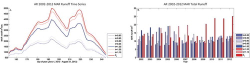
Choice of watershed generation method is particularly important for SMB runoff studies that estimate the amount of meltwater produced by a given watershed (Figure 4). For example, for the AR land-ice watershed, we find that annual total MAR SMB runoff for 2002–2012 for hydraulic potential watersheds with k = 1 ranges from 9.04 to 19.09 km³, while the runoff from Z_i land-ice watersheds ranges from 12.15 to 25.14 km³. For the same time period, MAR runoff in PK and MK hydraulic potential land-ice watersheds with k = 1 ranges between 2.14–9.60 km³ and 3.20–12.68 km³, respectively.

Figure 4. The MAR modeled runoff for different Aussivigssuit River (AR) land-ice watersheds for hydraulic potential with k-values varying between k = 0.80 and k = 1.10 and surface DEM methods is calculated for all years between 2002 and 2012. (A) Plots the MAR runoff daily time series for each watershed configuration during the 2012 melt season (1 June 2012 through 31 August 2012). (B) Denotes the total annual MAR runoff for each watershed configuration (similar to Lindbäck et al. 2015).

Furthermore, we find that variations in / have a strong influence on total runoff variability. For example, in 2008, one of the years with relatively low total SMB runoff, the hydraulic potential watershed with k = 0.95 is found to produce 14.29 km³ of runoff, the most of any watershed variant in that year. Comparatively, the watershed with k = 0.85 is found to produce 8.49 km³ of runoff, the least of any watershed variant in 2008. Thus, in the AR land-ice watershed in 2008, varying / results in a 5.8 km³ range in total MAR SMB runoff due solely to variations in watershed generation method and k-value selection (Figure 4). Given the absence of available in situ data for direct k-value calibration, we recommend using a multi-watershed approach with a spectrum of potential solutions for constraining GrIS modeled runoff estimates.

5. Discussion and conclusions

The CryoSheds modeling framework presented here offers new utility to the GrIS science community that currently lacks a standard procedure for generating land-ice watersheds that route meltwater to a user defined proglacial pour point. There does not appear to be an algorithmic explanation for differences observed between hydraulic potential with k = 1 and Z_i land-ice watersheds; but they are unsurprising as the two approaches simulate different physical processes. Two possible explanations are (1) differences in root data sources between Z_i and Z_b DEMs, which may cause grid disagreements when the two datasets are merged into a hydraulic pressure grid and results are compared with the Z_i DEM watersheds and (2) bedrock topography may be sufficiently steep relative to the surface topography, such that the hydraulic potential watershed divides are dominated by bedrock rather than surface topography.

It is also important to make note of other methods that are used to resolve glacier watersheds. For example, both Bolch, Menounos, and Wheate (2010) and Kienholz, Hock, and Arendt (2013) establish algorithms that use GIS-based watershed modeling tools that are used to inventory glaciers in Alaska and Canada. Pfeffer et al. (2014) apply these algorithms to assist in generating a global inventory of glaciers outside of the polar ice sheets. While noteworthy, these algorithms differ from CryoSheds in a number of ways. In particular, CryoSheds (1) offers an integrated solution that accounts for subglacial drainage; (2) offers an integrated solution that accounts for changes in subglacial pressures (k); (3) aggregates ice subbasins using glacier outflow and hydrologic flow directions; and (4) delineates contributing hydrologic areas from flexibly located, user-defined proglacial pour points.

There are also two key GrIS-specific watershed delineation techniques that, in part, provide a foundation for CryoSheds and are important to discuss. First, Banwell, Willis, and Arnold (2013) develop a distributed hydrologic model that routes water to the ice edge for a glacier in Northwest Greenland. A central contribution of this work that CryoSheds builds up is that k = 1 is not necessarily an optimal steady-state solution and thus variation in k should be considered. Second, Lindbäck et al. (2015) similarly compare modeled GrIS meltwater runoff with observed proglacial river outflow for neighboring land-terminating glaciers in Western Greenland, also using the hydraulic potential method. They vary k and find evidence that subglacial drainage pathways switch between neighboring glaciers seasonally and attribute this switching to changes in subglacial water pressure. Both of these studies rely on proglacial river discharge for calibration and validation of k. However, such field data in Greenland are scarce and thus is not practical for a semi-automated watershed algorithm like CryoSheds. Therefore, we submit that the important contributions of CryoSheds are in its GIS-based innovations to enable: (1) flexible location of user-defined proglacial pour points from which contributing land and ice watershed areas can be mapped, (2) seamless integration of subglacial water pressure variabilities, and (3) an ice subbasin merging technique that is based both on glacier outflow locations and DEM-derived hydrologic flow directions.

In conclusion, the CryoSheds modeling framework offers a flexible, standardized toolkit for generating watersheds for cryo-hydrologic systems. The nontrivial differences between the surface DEM and hydraulic potential approaches observed in these demonstrations suggest that future research should incorporate additional empirical datasets, particularly hydrologic outflow in proglacial rivers to determine which approach and ranges of k are reasonable for the purpose of delineating cryo-hydrologic watersheds for the GrIS. Until then, we suggest considering multiple watershed types simultaneously as end-member possibilities (as generated here using CryoSheds), in favor of any single delineation alone.

Acknowledgments

This work was supported by NASA Cryosphere [NNX14AH93G]; NASA Earth and Space Science Fellowship (NESSF) [NNX14AP57H]; UCLA Graduate Research Mentorship Program. Vena Chu and Jida Wang kindly provided important critical comments and suggestions at different stages of this research. We also thank the contributions of two anonymous reviewers and Prof. Graham Cogley whose thorough comments and detailed reviews helped greatly improve this work.

Disclosure statement

No potential conflict of interest was reported by the authors.

Supplemental data

Supplemental data for this article can be accessed here.

Additional information

Funding

This work was supported by NASA Cryosphere [NNX14AH93G]; NASA Earth and Space Science Fellowship (NESSF) [NNX14AP57H]; UCLA Graduate Research Mentorship Program.

References

- Bamber, J. L., M. J. Siegert, J. A. Griggs, S. J. Marshall, and G. Spada. 2013. “Paleofluvial Mega-Canyon Beneath the Central Greenland Ice Sheet.” Science 341 (6149): 997–999. doi:10.1126/science.1239794.
- Band, L. E. 1986. “Topographic Partition of Watersheds with Digital Elevation Models.” Water Resources Research 22 (1): 15–24. doi:10.1029/WR022i001p00015.
- Band, L. E., C. L. Tague, S. E. Brun, D. E. Tenenbaum, and R. A. Fernandes. 2000. “Modelling Watersheds as Spatial Object Hierarchies: Structure and Dynamics.” Transactions in GIS 4 (3): 181–196. doi:10.1111/1467-9671.00048.
- Banwell, A. F., I. C. Willis, and N. S. Arnold. 2013. “Modeling Subglacial Water Routing at Paakitsoq, W Greenland.” Journal of Geophysical Research: Earth Surface 118 (3): 1282–1295. doi:10.1002/jgrf.20093.
- Bartholomew, I., P. Nienow, A. Sole, D. Mair, T. Cowton, S. Palmer, and J. Wadham. 2011. “Supraglacial Forcing of Subglacial Drainage in the Ablation Zone of the Greenland Ice Sheet.” Geophysical Research Letters 38 (8). doi:10.1029/2011GL047063.
- Bjornsson, H. 1986. “Delineation Of Glacier Drainage Basins On Western Vatnajokull.” Annals of Glaciology 8: 19–21.
- Bolch, T., B. Menounos, and R. Wheate. 2010. “Landsat-Based Inventory of Glaciers in Western Canada, 1985–2005.” Remote Sensing of Environment 114 (1): 127–137. doi:10.1016/j.rse.2009.08.015.
- Box, J. E., and D. H. Bromwich. 2004. “Greenland Ice Sheet Surface Mass Balance 1991–2000: Application of Polar MM5 Mesoscale Model and in Situ Data.” Journal of Geophysical Research 109 (D16). doi:10.1029/2003JD004451.
- Chandler, D. M., J. L. Wadham, G. P. Lis, T. Cowton, A. Sole, I. Bartholomew, J. Telling, et al. 2013. “Evolution of the Subglacial Drainage System beneath the Greenland Ice Sheet Revealed by Tracers.” Nature Geoscience 6 (3): 195–198. doi:10.1038/ngeo1737.
- Chu, W., T. T. Creyts, and R. E. Bell. 2016. “Rerouting of Subglacial Water Flow between Neighboring Glaciers in West Greenland: Subglacial Flow Rerouting in Greenland.” Journal of Geophysical Research: Earth Surface. doi:10.1002/2015JF003705.
- Cowton, T., P. Nienow, I. Bartholomew, A. Sole, and D. Mair. 2012. “Rapid Erosion beneath the Greenland Ice Sheet.” Geology 40 (4): 343–346. doi:10.1130/G32687.1.
- Cowton, T., P. Nienow, A. Sole, J. Wadham, G. Lis, I. Bartholomew, D. Mair, and D. Chandler. 2013. “Evolution of Drainage System Morphology at a Land-Terminating Greenlandic Outlet Glacier.” Journal of Geophysical Research: Earth Surface 118 (1): 29–41. doi:10.1029/2012JF002540.
- Cuffey, K., and W. S. B. Paterson. 2010. The Physics of Glaciers. 4th ed. Burlington, MA: Butterworth-Heinemann.
- Fitzpatrick, A. A. W., A. L. Hubbard, J. E. Box, D. J. Quincey, D. van As, A. P. B. Mikkelsen, S. H. Doyle, C. F. Dow, B. Hasholt, and G. A. Jones. 2014. “A Decade (2002–2012) of Supraglacial Lake Volume Estimates across Russell Glacier, West Greenland.” The Cryosphere 8 (1): 107–121. doi:10.5194/tc-8-107-2014.
- Flowers, G. E., and G. K. C. Clarke. 1999. “Surface and Bed Topography of Trapridge Glacier, Yukon Territory, Canada: Digital Elevation Models and Derived Hydrauli c Geometry.” Journal of Glaciology 45 (149): 165–174.
- Hanna, E., P. Huybrechts, I. Janssens, J. Cappelen, K. Steffen, and A. Stephens. 2005. “Runoff and Mass Balance of the Greenland Ice Sheet: 1958–2003.” Journal of Geophysical Research 110: D13. doi:10.1029/2004JD005641.
- Harper, J., N. Humphrey, W. T. Pfeffer, J. Brown, and X. Fettweis. 2012. “Greenland Ice-Sheet Contribution to Sea-Level Rise Buffered by Meltwater Storage in Firn.” Nature 491 (7423): 240–243. doi:10.1038/nature11566.
- Hasholt, B., S. A. Khan, and A. B. Mikkelsen. 2014. “GPS Based Surface Displacements – a Proxy for Discharge and Sediment Transport from the Greenland Ice Sheet.” The Cryosphere Discussions 8 (4): 3829–3850. doi:10.5194/tcd-8-3829-2014.
- Hasholt, B., A. B. Mikkelsen, M. H. Nielsen, and M. A. Larsen. 2013. “Observations of Runoff and Sediment and Dissolved Loads from the Greenland Ice Sheet at Kangerlussuaq, West Greenland, 2007 to 2010.” Zeitschrift Für Geomorphologie, Supplementary Issues 57 (2): 3–27. doi:10.1127/0372-8854/2012/S-00121.
- Howat, I. M., A. Negrete, and B. E. Smith. 2014. “The Greenland Ice Mapping Project (GIMP) Land Classification and Surface Elevation Data Sets.” The Cryosphere 8 (4): 1509–1518. doi:10.5194/tc-8-1509-2014.
- Jenson, S. K., and J. O. Domingue. 1988. “Extracting Topographic Structure from Digital Elevation Data for Geographic Information-System Analysis.” Photogrammetric Engineering and Remote Sensing 54 (11): 1593–1600.
- Kienholz, C., R. Hock, and A. A. Arendt. 2013. “A New Semi-Automatic Approach for Dividing Glacier Complexes into Individual Glaciers.” Journal of Glaciology 59 (217): 925–937. doi:10.3189/2013JoG12J138.
- Lewis, S. M., and L. C. Smith. 2009. “Hydrologic Drainage of the Greenland Ice Sheet.” Hydrological Processes 23 (14): 2004–2011. doi:10.1002/hyp.7343.
- Lindbäck, K., R. Pettersson, A. L. Hubbard, S. H. Doyle, D. van As, A. B. Mikkelsen, and A. A. Fitzpatrick. 2015. “Subglacial Water Drainage, Storage, and Piracy beneath the Greenland Ice Sheet.” Geophysical Research Letters 42 (18): 7606–7614. doi:10.1002/2015GL065393.
- Luo, H., R. M. Castelao, A. K. Rennermalm, M. Tedesco, A. Bracco, P. L. Yager, and T. L. Mote 2016. “Oceanic Transport of Surface Meltwater from the Southern Greenland Ice Sheet.” Nature Geoscience. doi:10.1038/ngeo2708.
- Marks, D., J. Dozier, and J. Frew. 1983. “Automated Basin Delineation from Digital Terrain Data.” NASA Goddard Space Flight Center.
- Mernild, S. H., and B. Hasholt. 2009. “Observed Runoff, Jökulhlaups and Suspended Sediment Load from the Greenland Ice Sheet at Kangerlussuaq, West Greenland, 2007 and 2008.” Journal of Glaciology 55 (193): 855–858. doi:10.3189/002214309790152465.
- Mernild, S. H., and G. E. Liston. 2012. “Greenland Freshwater Runoff. Part II: Distribution and Trends, 1960–2010.” Journal of Climate 25 (17): 6015–6035. doi:10.1175/JCLI-D-11-00592.1.
- Mernild, S. H., G. E. Liston, C. A. Hiemstra, J. H. Christensen, M. Stendel, and B. Hasholt. 2011. “Surface Mass Balance and Runoff Modeling Using HIRHAM4 RCM at Kangerlussuaq (Søndre Strømfjord), West Greenland, 1950–2080.” Journal of Climate 24 (3): 609–623. doi:10.1175/2010JCLI3560.1.
- Mernild, S. H., G. E. Liston, K. Steffen, M. van den Broeke, and B. Hasholt. 2010. “Runoff and Mass-Balance Simulations from the Greenland Ice Sheet at Kangerlussuaq (Søndre Strømfjord) in a 30-Year Perspective, 1979–2008.” The Cryosphere 4 (2): 231–242. doi:10.5194/tc-4-231-2010.
- Mernild, S. H., G. E. Liston, and M. van den Broeke. 2012. “Simulated Internal Storage Buildup, Release, and Runoff from Greenland Ice Sheet at Kangerlussuaq, West Greenland.” Arctic, Antarctic, and Alpine Research 44 (1): 83–94. doi:10.1657/1938-4246-44.1.83.
- Mikkelsen, A. B., B. Hasholt, N. T. Knudsen, and M. H. Nielsen. 2013. “Jökulhlaups and Sediment Transport in Watson River, Kangerlussuaq, West Greenland.” Hydrology Research 44 (1): 58. doi:10.2166/nh.2012.165.
- Moore, G. K., L. G. Baten, G. J. Allord, and C. J. Robinove. 1983. “Application of Digital Mapping Technology to the Display of Hydrologic Information; a Proof-of-Concept Test in the Fox-Wolf River Basin, Wisconsin.” Report 83–4142. Water-Resources Investigations Report. USGS. USGS Publications Warehouse. http://pubs.er.usgs.gov/publication/wri834142
- Morlighem, M., E. Rignot, J. Mouginot, H. Seroussi, and E. Larour. 2014. “Deeply Incised Submarine Glacial Valleys Beneath the Greenland Ice Sheet.” Nature Geoscience 7 (6): 418–422. doi:10.1038/ngeo2167.
- Morlighem, M., E. Rignot, J. Mouginot, H. Seroussi, and E. Larour. 2015. IceBridge BedMachine Greenland, Version 2, Bedrock Altitude, Ice Surface Elevation, Ice Thickness Mask. Boulder, CO: NASA DAAC at the National Snow and Ice Data Center. doi:10.5067/AD7B0HQNSJ29.
- Morlighem, M., E. Rignot, H. Seroussi, E. Larour, H. Ben Dhia, and D. Aubry. 2011. “A Mass Conservation Approach for Mapping Glacier Ice Thickness.” Geophysical Research Letters 38 (19): n/a-n/a. doi:10.1029/2011GL048659.
- Noh, M.-J., and I. M. Howat. 2015. “Automated Stereo-Photogrammetric DEM Generation at High Latitudes: Surface Extraction with TIN-Based Search-Space Minimization (SETSM) Validation and Demonstration over Glaciated Regions.” GIScience & Remote Sensing 52 (2): 198–217. doi:10.1080/15481603.2015.1008621.
- O’Callaghan, J. F., and D. M. Mark. 1984. “The Extraction of Drainage Networks from Digital Elevation Data.” Computer Vision, Graphics, and Image Processing 28 (3): 323–344. doi:10.1016/S0734-189X(84)80011-0.
- Overeem, I., B. Hudson, E. Welty, A. Mikkelsen, J. Bamber, D. Petersen, A. Lewinter, and B. Hasholt. 2015. “River Inundation Suggests Ice-Sheet Runoff Retention.” Journal of Glaciology 61 (228): 776–788. doi:10.3189/2015JoG15J012.
- Palmer, S., A. Shepherd, P. Nienow, and I. Joughin. 2011. “Seasonal Speedup of the Greenland Ice Sheet Linked to Routing of Surface Water.” Earth and Planetary Science Letters 302 (3–4): 423–428. doi:10.1016/j.epsl.2010.12.037.
- Pfeffer, W. T., A. A. Arendt, A. Bliss, T. Bolch, J. G. Cogley, A. S. Gardner, J.-O. Hagen, et al. 2014. “The Randolph Glacier Inventory: A Globally Complete Inventory of Glaciers.” Journal of Glaciology 60 (221): 537–552. doi:10.3189/2014JoG13J176.
- Rennermalm, A. K., L. C. Smith, V. W. Chu, J. E. Box, R. R. Forster, M. R. van den Broeke, D. van As, and S. E. Moustafa. 2013. “Evidence of Meltwater Retention Within the Greenland Ice Sheet.” The Cryosphere 7 (5): 1433–1445. doi:10.5194/tc-7-1433-2013.
- Rennermalm, A. K., L. C. Smith, V. W. Chu, S. E. Moustafa, L. H. Pitcher, and C. J. Gleason. 2014. “Proglacial River Dataset from the Akuliarusiarsuup Kuua River Northern Tributary, Southwest Greenland, 2008-2013, Version 2.0.” Pangaea. doi:10.1594/PANGAEA.838812.
- Rignot, E., I. Velicogna, M. R. van den Broeke, A. Monaghan, and J. T. M. Lenaerts. 2011. “Acceleration of the Contribution of the Greenland and Antarctic Ice Sheets to Sea Level Rise.” Geophysical Research Letters 38 (5): n/a-n/a. doi:10.1029/2011GL046583.
- Rippin, D., I. Willis, N. Arnold, A. Hodson, J. Moore, J. Kohler, and H. BjöRnsson. 2003. “Changes in Geometry and Subglacial Drainage of Midre Lovénbreen, Svalbard, Determined from Digital Elevation Models: Changes in glacier geometry from dems.” Earth Surface Processes and Landforms 28 (3): 273–298. doi:10.1002/esp.485.
- Shreve, R. L. 1972. “Movement of Water in Glaciers.” Journal of Glaciology 11 (62): 205–214.
- Smith, L. C., V. W. Chu, K. Yang, C. J. Gleason, L. H. Pitcher, A. K. Rennermalm, C. J. Legleiter, et al. 2015. “Efficient Meltwater Drainage through Supraglacial Streams and Rivers on the Southwest Greenland Ice Sheet.” Proceedings of the National Academy of Sciences 112 (4): 1001–1006. doi:10.1073/pnas.1413024112.
- Tarboton, D. G., R. L. Bras, and I. Rodriguez-Iturbe. 1991. “On the Extraction of Channel Networks from Digital Elevation Data.” Hydrological Processes 5 (1): 81–100. doi:10.1002/hyp.3360050107.
- Tedesco, M., X. Fettweis, and P. Alexander. 2013. MAR v3.2 Regional Climate Model Data for Greenland (1958-2013). NSF Arctic Data Center. doi:10.5065/D6JH3J7Z.
- Vernon, C. L., J. L. Bamber, J. E. Box, M. R. van den Broeke, X. Fettweis, E. Hanna, and P. Huybrechts. 2013. “Surface Mass Balance Model Intercomparison for the Greenland Ice Sheet.” The Cryosphere 7 (2): 599–614. doi:10.5194/tc-7-599-2013.
- Yang, K., L. C. Smith, V. W. Chu, C. J. Gleason, and M. Li. 2015. “A Caution on the Use of Surface Digital Elevation Models to Simulate Supraglacial Hydrology of the Greenland Ice Sheet.” IEEE Journal of Selected Topics in Applied Earth Observations and Remote Sensing 8 (11): 5212–5224. doi:10.1109/JSTARS.2015.2483483.
- Yang, K., L. C. Smith, V. W. Chu, L. H. Pitcher, C. J. Gleason, A. K. Rennermalm, and M. Li. 2016. “Fluvial Morphometry of Supraglacial River Networks on the Southwest Greenland Ice Sheet.” GIScience & Remote Sensing 53 (4): 459–482. doi:10.1080/15481603.2016.1162345.
- Yde, J. C., N. T. Knudsen, B. Hasholt, and A. B. Mikkelsen. 2014. “Meltwater Chemistry and Solute Export from a Greenland Ice Sheet Catchment, Watson River, West Greenland.” Journal of Hydrology 519: 2165–2179. doi:10.1016/j.jhydrol.2014.10.018.