Curve matching approaches to waveform classification: a case study using ICESat data

Abstract

Light Detection and Ranging (LiDAR) waveforms are being increasingly used in many forest and urban applications, especially for ground feature classification. However, most studies relied on either discretizing waveforms to multiple returns or extracting shape metrics from waveforms. The direct use of the full waveform, which contains the most comprehensive and accurate information has been scarcely explored. We proposed to utilize the complete waveform to test its ability to differentiate between objects having distinct vertical structures using curve matching approaches. Two groups of curve matching approaches were developed by extending methods originally designed for pixel-based hyperspectral image classification and object-based high spatial image classification. The first group is based on measuring the curve similarity between an unknown waveform and a reference waveform, including curve root sum squared differential area (CRSSDA), curve angle mapper (CAM), and Kullback–Leibler (KL) divergence. The second group assesses the curve similarity between an unknown and reference cumulative distribution functions (CDFs) of their waveforms, including cumulative curve root sum squared differential area (CCRSSDA), cumulative curve angle mapper (CCAM), and Kolmogorov–Smirnov (KS) distance. When employed to classify open space, trees, and buildings using ICESat waveform data, KL provided the highest average classification accuracy (87%), closely followed by CCRSSDA and CCAM, and they all significantly outperformed KS, CRSSDA, and CAM based on 15 randomized sample sets.

Keywords:

• waveform
• classification
• curve matching
• ICESat/GLAS

1. Introduction

Light Detection and Ranging (LiDAR) is an active remote sensing technology which uses visible, near-infrared, or shortwave infrared laser beams to measure ground elevation, while also providing information on the vertical structure of geographical objects. There are two types of LiDAR data: discrete-return LiDAR and full-waveform LiDAR (Ussyshkin and Theriault 2011). Currently, discrete-return LiDAR data are the mainstream commercial product and a great number of off-the-shelf tools are available for processing discrete-return LiDAR (Ussyshkin and Theriault 2011). Up to six returns per transmitted laser pulse are typically recorded, and these typically have x, y, elevation, and intensity measured for each (Sasaki et al. 2012; Zhou 2013).

Full waveform, a relatively new LiDAR product, records the quasi-continuous time-varying strength of the return signal from the illuminated area (called the waveform footprint) using small time intervals (e.g. 1 nanosecond). Waveform LiDAR has become increasingly popular in the last decade and it is able to provide thousands of measurements for each transmitted laser pulse (Mallet et al. 2011; Ussyshkin and Theriault 2011; Alexander et al. 2010). Since waveform data provide finer vertical resolution, they offer an enhanced capability to reflect the vertical structures of geographical objects (Wagner et al. 2008; Farid et al. 2008). The shape of a waveform is the result of interaction between the transmitted laser pulse and intercepted object surfaces within the footprint (Alexander et al. 2010; Pirotti 2010). For example, waveforms over trees are influenced by characteristics such as tree density, structure, and vegetation phase. Given that discrete-return LiDAR provides no more than six measurements in its vertical profile which may be separated by a few meters in vertical distance, LiDAR waveform provides a better 3D profile of an object (Ussyshkin and Theriault 2011).

Because of free availability, regular repetition, and global coverage, the large-footprint waveform data from the Geoscience Laser Altimeter System (GLAS) onboard the Ice, Cloud, and land Elevation Satellite (ICESat) have been widely used. Previous applications especially focused on forest studies (Harding and Carabajal 2005; Lee et al. 2011; Sun et al. 2008; Lefsky et al. 2007; Wang et al. 2012) and building model reconstruction in urban environments (Gong et al. 2011; Cheng et al. 2011). For these studies, the first step usually involves identifying waveforms over trees or buildings and separating them from those over other land cover classes. These analyses can be very time-consuming and labor-intensive because the first step is usually achieved through visual interpretation (sometimes with the aid of existing land use land cover information) (Gong et al. 2011; Cheng et al. 2011). Our previous study has demonstrated the ability of full waveforms alone to differentiate between trees, buildings, and open space using a Kolmogorov–Smirnov (KS) distance-based curve matching approach (Zhou et al. 2015), which outperformed the widely used metrics-based approach. This current study is a continuing effort on curve matching approach-based research, but with a focus on the comparison of different curve matching approaches that we developed for waveform classification. If these approaches are demonstrated to be successful, they could be potentially used to improve the research in forest and urban studies that primarily employ 2D remotely sensed imagery by incorporating the vertical structure information that the waveforms provide.

2. Background

In general, a LiDAR waveform may have one or many echoes, where one echo is a peak that corresponds to an individual target encountered or a cluster of objects too close to be separated, while multiple echoes often represent either multiple targets or one target with multiple components that are vertically separable within the footprint (Alexander et al. 2010). Consequently, the shapes of waveforms over multiple objects can be very complex. To perform waveform classification, existing studies have relied on simplifying the complex waveform data based on either the discretization of the full waveform into multiple returns or the derivation of metrics to characterize the waveform shapes. A large number of studies have attempted to extract more returns from full waveforms through discretization to overcome the limitations of discrete-return LiDAR, which has only a few returns and fails to adequately capture the vertical structures of geographical objects (Wagner et al. 2008; Rutzinger et al. 2008; Mallet et al. 2011; Reitberger et al. 2009; Mallet and Bretar 2009; Ussyshkin and Theriault 2011; Guo et al. 2011). Discretization of full waveform offers flexibility in that the number of returns extracted can be determined by users (Ussyshkin and Theriault 2011). The number of resultant returns can be set to be many more than that of the traditional discrete- return LiDAR. The larger number of extracted returns can better represent the vertical structure of objects. Comparatively, the number of discretized returns is also significantly less than that of the original full waveform. With manageable complexity, the discretized returns can then be analyzed by algorithms designed for traditional discrete-return LiDAR.

To avoid dealing with the complex shape of a waveform, other studies have utilized waveform-derived summary metrics such as the number of echoes, peak amplitude, echo width, skewness, and kurtosis to represent key characteristics of the waveform’s shapes (Molijn, Lindenbergh, and Gunter 2011; Mallet et al. 2011). These metrics have had varied success in differentiating land cover types. As with the discretization of waveforms, these waveform-derived metrics simplify the complexity of the complete waveforms, in this case by focusing on important shape characteristics. However, by reducing complexity, both the discretization of waveforms into multiple returns and the derivation of shape-related metrics are unable to take advantage of the entirety of information that the full waveform offers.

The complete curve of a full waveform contains substantially more information than the discretized returns or summary metrics extracted from the waveform. However, the complete waveform curves have rarely been utilized to perform classification because of the lack of appropriate approaches for dealing with their complexity. In an earlier paper (Zhou et al. 2015), we proposed a curve matching approach to directly compare waveform curves using KS distance as an alternative to the methods based on the simplification of waveforms. Preliminary results showed that this approach outperformed a widely adopted metrics-based method using waveform-derived metrics. This result suggested that curve matching approaches to waveform classification is a new direction worth in-depth exploration.

In fact, curve matching approaches are not unfamiliar to remote sensing community since they have been utilized for both pixel-based hyperspectral image classification and object-based image classifications. For pixel-based hyperspectral image classification, a spectral signature is a curve of reflectance values across an electromagnetic spectrum (Jensen 2004). The shape of a hyperspectral curve is determined by the absorptive characteristics of the material. Various methods have been developed to assess the similarity of the hyperspectral curves of pixels with those of different materials in a spectral library for identification and classification purposes, such as the spectral angle mapper (SAM) (Kruse et al. 1993), root sum squared differential area (RSSDA) (Hamada et al. 2007), and Kullback–Leibler (KL) divergence (Chang 2000).

For object-based image classification, the frequency distribution function (histogram) and cumulative distribution function (CDF) of the pixel values within an image object for a particular band were used to perform object-based feature extraction using methods extended from existing pixel-based hyperspectral image classification (Stow et al. 2012; Toure et al. 2013; Sridharan and Qiu 2013; Zhou and Qiu 2015). For example, Stow et al. (2012) proposed a Histogram Matching Root Sum Squared Differential Area (HMRSSDA) method, which was extended from the RSSDA approach (Hamada et al. 2007), to measure the similarity of object-level histogram curves for land cover and land use classification. Continuing the work of Stow et al. (2012), Toure et al. (2013) extended the SAM approach (Kruse et al. 1993) to develop a Histogram Angle Mapper (HAM) to measure the similarity of object-based histograms. Both HMRSSDA and HAM classifiers have consistently outperformed the widely adopted nearest neighbor object-based classifiers. We also developed a fuzzy KS-based classifier to assess the similarity of the reflectance values in an unknown object compared to those in a known object by using the CDF rather than the frequency histogram distribution. This approach achieved more than 10% improvements over other popular object- and pixel-based classifiers (Sridharan and Qiu 2013). Recently, we developed a KL divergence-based classifier to quantify the similarity of object-level histogram curves, which performed significantly better than HAM and HMRSSDA, though not significantly better than the KS classifier (Zhou and Qiu 2015).

A waveform is not only a curve but also can be considered as a time-varying frequency distribution function or histogram (Muss, Mladenoff, and Townsend 2011). Therefore, it is intuitive to extend both pixel-based hyperspectral image classification methods and object-based high spatial image classification approaches to waveform curves. Aside from the KS-based curve matching approach we presented in Zhou et al. (2015), we are unaware of other studies using curve matching approaches to classify complete waveforms. In this study, we developed and explored two groups of curve matching approaches by extending methods originally designed for pixel-based hyperspectral image classification or object-based high spatial image classification. The first group was designed to measure the curve similarity between an unknown waveform and reference waveform, including curve root sum squared differential area (CRSSDA), curve angle mapper (CAM), and the KL divergence. The second group was developed to assess the curve similarity between an unknown and a reference CDFs of their waveforms, including cumulative curve root sum squared differential area (CCRSSDA), cumulative curve angle mapper (CCAM), and the KS distance.

3. Study area and data

The study area is located in Dallas, Texas, bounded approximately by 97.031–96.518° W in longitude and 32.553–32.996° N in latitude. The area is characterized by a mixture of mature residential neighborhoods, and commercial and industrial buildings. ICESat waveforms are sensitive to surface terrain due to their large footprints. Since the majority of the study area is flat (slope ≤10°), the terrain is not expected to significantly influence the waveform shapes (Gong et al. 2011; Hilbert and Schmullius 2012; Duong et al. 2009) and the resulting classification.

Due to the large spacing between its footprints, ICESat waveform has not been widely used for operational land cover mapping, which usually requires contiguous coverage of the study area. However, intent of this study is to evaluate the effectiveness of the curve matching approaches for waveform classification by capitalizing the vertical structure information embedded in the data. ICESat data is employed here as a case study for the developed approaches. If proved effective, these approaches could be readily applied to other LiDAR waveform data with contiguous coverages, such as those from airborne systems.

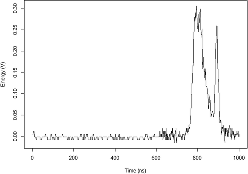
The ICESat program distributes 15 Level-1 and Level-2 data products (ranging from GLA01 to GLA15), which can be downloaded from the website of the National Snow and Ice Data Center (http://nsidc.org/data/icesat/data.html). The full waveform data were extracted from GLA01 (L1A Global Altimeter Data), the footprint shape information were calculated using the parameters in GLA05 (L1B global waveform-based range correction data), and the center location of the waveform footprints were derived from GLA14 (L2A Global Land Surface Altimetry Data). All datasets were linked by their common index and shot number. Figure 1 is an example of ICESat waveform over an area with trees.

Figure 1. An example of ICESat waveform over an area of trees.

ICESat footprints are elliptical in shape and their sizes vary from 50 to 150 m with an average size around 75 m. The approximate areas of the waveform footprints were computed using the method proposed by Gong et al. (2011). The resulting waveform footprint polygons were then converted to keyhole markup language (KML) and imported to Google Earth. The land cover conditions within the selected footprints were determined through visual interpretation of the Google Earth image. We used three general land cover categories with distinct vertical structures: buildings, trees, and open spaces. All land cover types with a flat open surface (e.g. bare land, water, roads, and parking lots) were assigned to the open space category. They were not identified as separate categories since they have generally similar vertical waveform curves, and it is very difficult to classify them using the waveform LiDAR alone. Similarly, there was no differentiation of building subtypes (such as residential or commercial), or tree subtypes (such as deciduous or coniferous). These very general land cover categories were a necessity because the large size of the ICESat footprint does not allow a more detailed level of classification (Zhou et al. 2015).

4. Methodology

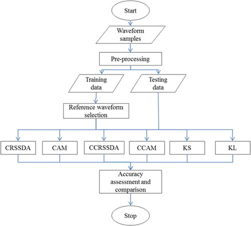
Curve matching approaches measure the curve similarity between two samples. One sample is usually with a known class (training sample) and the class of the other is predicted (testing sample). For this purpose, after applying a set of preprocessing procedures, the waveform dataset was divided into training and testing subsets. To compare the six proposed curve matching approaches, the performance difference between any two curve matching approaches was assessed with the pairwise McNemar’s chi-square significance test. The test was based on 15 randomly selected reference waveform sets, each with a total of 54 reference waveforms, comprising 19 reference waveforms for buildings, 24 for trees, and 11 for open space. The methodological steps required for this study are summarized in the flow chart in Figure 2.

Figure 2. General flowchart of methodology.

4.1. Preprocessing

A number of preprocessing steps were needed to make the waveform data suitable for the subsequent analysis. First, both GLA01 and GLA14 were converted from distributed binary format to ASCII format, and the unit of GLA01 was converted from count (0–255) to voltage. Then, the ellipsoid of GLA14 was transformed from the default TOPEX/Poseidon to the WGS84 coordinate system to match reference data. Second, unreliable outlier waveforms, such as those with a reflectivity lower than 0.1(Molijn, Lindenbergh, and Gunter 2011), or those with a signal-to-noise ratio lower than 10 (Hilbert and Schmullius 2012), were excluded because they were primarily caused by dense cloud. Finally, a noise removal procedure was applied to eliminate system noise at the beginning and end of each waveform signal. Any waveform signal value below the threshold was regarded as noise and was assigned a value of zero. The threshold was determined using the method proposed by Lefsky et al. (2007). The starting location of a waveform was defined by finding the farthest left location of the waveform where the signal was larger than the threshold value, and the ending location was identified by the rightmost location where the signal was larger than the threshold value. The earliest starting location of the reliable waveforms was the 651st ns, and the last ending location was close to the 1000th ns value (Zhou et al. 2015). Therefore, only signals over the last 350 ns (from 651st to 1000th ns) were analyzed in this study.

After preprocessing, only waveforms having a dominant type were identified as samples for each class in this study because the waveform shapes were primarily influenced by the vertical structures of the dominant land cover type within the footprints. This was relatively easy to achieve for the open space category due to common presence of large open spaces in Dallas. However, due to the likely presence of bare land, grass with a mixture of buildings and trees inside the large ICESat footprints, only waveforms where buildings or trees covered more than 50% of the area based on Google Earth image were considered as buildings or trees, respectively. The waveform footprints that did not have a single dominant land cover type, but instead had a mixture of several dominant types with none exceeding 50% in coverage were excluded from the training and testing processes because they could not be easily labeled with a single class in a hard classification such as the one used in this study. Like a mixed pixel, the classification of mixed footprints should be investigated using a fuzzy classification algorithm in the future, which, however, is not the focus of this study. If the potential of waveform curves using curve matching approaches can be demonstrated, the same methods could be extended to small footprint airborne LiDAR by segmenting point clouds or image into objects first and then synthesizing object-level pseudo-waveforms using a histogram of discrete LiDAR returns or waveforms (Zhou and Qiu 2015). Since the footprints of these objects are derived from HSR imagery through image segmentation, the mixed footprint problem would not be an issue anymore because each image segment usually has a dominant land cover type as a result of segmentation. When all the samples were identified for each class, around half of the samples for each class were randomly separated as training samples and the other half as testing samples, as shown in Table 1.

Table 1. Number of training and testing samples.

Class	No. of training samples	No. of testing samples
Building	91	92
Tree	135	135
Open space	195	196

4.2. Reference waveform selection

For the majority of existing curve matching-based classifications, each class is assumed to have a single end-member or reference sample. An end-member/reference is one of the training samples that is identified to represent relatively pure material (Jensen 2004) or is obtained by averaging all the training samples (Ghiyamat et al. 2013; Stow et al. 2012; Toure et al. 2013). This approach is meaningful when differences among the curves within the same class (within-class variation) are negligible. However, the training dataset here has a high-degree of within-class variation, especially for the tree and the building classes. This is due to varied height levels, vertical structures, or net coverages within the footprints. As a consequence, using a single end-member/reference sample is not appropriate. For complexity and resource reasons, it is also not appropriate to use all the training samples as reference waveforms since many waveforms in a training class have similar profiles. Instead, a subset of reference waveforms needs to be selected for each class. This should provide better discrimination ability than using a single end-member due to the capturing of within-class variation of the training data (Cho et al. 2010; Ghiyamat et al. 2013), while avoiding the complexity and data duplication associated with the use of all training waveforms as references.

In our previous study (Zhou et al. 2015), a principal component analysis (PCA) was used to select a small number of references from the training dataset. This avoided data duplication while also reflecting within-class variation. However, it is not appropriate in the current context to use PCA-selected reference waveforms to evaluate the performance of the six proposed curve matching approaches. The PCA-based reference selection used KS distance to measure the curve similarity when selecting references. The references selected using the KS distance may favor the performance of the KS-based approach over the other five curve matching approaches when the actual classification is performed. Therefore, to avoid biasing any of the six curve matching approaches, the reference waveform selection process should not utilize any similarity measure that is employed for subsequent classification.

For this reason, the reference waveforms were simply randomly selected from the training dataset. Our previous study (Zhou et al. 2015) showed that 10 sets of randomly selected references were able to produce results with an average overall accuracy of 82% using the KS-based approach. To increase the representativeness of the random samples, we introduced additional random sample sets in this study. Each time when a new random sample set was introduced, the average overall accuracy was calculated over all the existing sample sets and was compared with the average overall accuracy of the previous iteration. The iteration stopped when the difference of the average overall accuracies was below 0.1% for two consecutive iterations, which indicated a stable average overall accuracy. As a result, a total of 15 sets of randomly selected reference waveforms were used to evaluate the final average performance of the six curve matching approaches. In order to maintain consistency with our earlier study, each set contained the same numbers of reference waveforms for each class as those determined by the PCA analysis in our previous study (Zhou et al. 2015).

4.3. Curve matching approaches

The classification of each testing waveform was accomplished by measuring the degree of curve similarity between the waveform and each in the randomly selected set of reference waveforms. Each testing waveform was assigned to the class of the reference waveform with the highest curve similarity. Generally, to calculate the curve similarity between two waveforms, let and be a reference waveform and a testing waveform respectively, each with n time bins (n = 350 in this study), and , be their corresponding CDFs. Each of six different curve matching measurements was used to assess the similarity between r and t, as follows.

4.3.1. Curve root sum squared differential area

CRSSDA is an area-based classifier that computes curve similarity by integrating the area between a testing waveform and a reference waveform. Similar to HMRSSDA (Stow et al. 2012), which was successfully used to match object-based histogram curves to differentiate between various image objects, CRSSDA is also extended from RSSDA (Hamada et al. 2007), which was originally designed for pixel-based hyperspectral classification. The method first calculates the squared difference between two waveform curves at each time bin, then sums the squared differences across all the bins, and finally computes the square root of the total squared difference to obtain waveform curve similarity (Equation (1)).

(1)

where min and max are the start and end location of the waveform. In this study, min equals 651 and max equals 1000, because only the signals from the 651st ns to the 1000th ns are considered. A smaller value of CRSSDA indicates a higher curve similarity between two waveforms.

Additionally, we generated the CDF curves of the waveforms and used these as inputs to Equation (1). We call this new approach CCRSSDA. The performance of CRSSDA and CCRSSDA was compared to see whether the CDF curve or the original waveform curve achieved better accuracy when the area-based approaches were used for waveform classification.

4.3.2. Curve angle mapper

As with HAM (Toure et al. 2013), the CAM approach is also extended from the SAM algorithm that was originally designed to quantify the curve similarity of hyperspectral pixels. The SAM algorithm compares the curve similarity of a testing spectral to a reference spectral by calculating the angle between and in n spectral dimensions using Equation (2). A smaller value of indicates a higher similarity between the two spectra. In this study, CAM is employed to measure the curve similarity between a testing waveform and a reference waveform using the same equation, where i refers to the i^th ns and n is the total number of bins. Theoretically, can vary from to , where stands for maximum similarity and stands for minimum similarity.

(2)

Similarly, when the CDF curves of waveforms are used as inputs to Equation (2), the method becomes a new approach named CCAM. The performance of CAM and CCAM was compared to determine which achieved better discrimination accuracy.

4.3.3. Kolmogorov–Smirnov distance

The KS distance is often used to measure curve similarity by calculating the maximum absolute distance between the CDFs of two frequency distributions, as described in Equation (3) (Burt and Barber 1996).

(3)

Since a waveform can be considered as a frequency distribution function (Zaletnyik, Laky, and Toth 2010), the CDF of the waveform was first generated and the KS distance was then calculated between each testing waveform and individual reference waveforms as in Zhou et al. (2015). The value of can vary from 0 to 1, where 0 indicates maximum similarity; while 1 indicates minimum similarity. KS distance can be applied to the CDFs but not their original waveforms.

4.3.4. Kullback–Leibler divergence

The KL divergence is another technique that measures curve similarity between two probability distribution functions (Kullback and Leibler 1951). It has been widely and successfully used in image pattern recognition (Olszewski 2012) and hyperspectral image classification (Ghiyamat et al. 2013). Since an object-level spectral histogram can be considered a probability distribution function, in Zhou and Qiu (2015) we developed a KL divergence approach to quantitatively measure the curve similarity between the spectral histogram of two objects. This achieved the highest classification accuracy compared with all other object-based curve matching approaches investigated. Since a waveform also can be normalized as a probability distribution function, we applied the KL divergence approach to measure the curve similarity between r and t using Equation (4).

(4)

A smaller value of indicates a higher curve similarity. Since KL divergence is only between two probability functions, we cannot apply it to the CDF of a waveform.

4.4. Accuracy assessment

The overall performance of each curve matching approach was evaluated in terms of total percentage accuracy. A pairwise McNemar’s chi-square test (Agresti 1996) was then conducted between each pair of approaches to evaluate if the improvement of one approach over the other was statistically significant for each of the 15 trials of randomly selected references.

Since each curve matching approach uses different scales or units, the resultant measures cannot be compared directly. To address this issue, all measures were normalized using a relative curve discriminatory probability (RCDPB) as in Equation (5). This was originally employed to evaluate the performance of different hyperspectral classification methods (Ghiyamat et al. 2013).

(5)

where represents the curve similarity between t and the ith reference waveform r using any one of the curve matching approaches and m is the number of selected reference waveforms. A smaller value of RCDPB indicates a higher curve similarity between two waveforms. RCDPB was used to assess and compare the performance of the six curve matching approaches for each of the classes.

5. Results and discussion

As explained earlier, 15 sets of randomly selected reference waveforms were used to evaluate the performance of the 6 curve matching approaches. In this section, the characteristics of the waveform curves were first examined using one set of randomly selected reference waveforms as an example. The relative performance of the 6 curve matching approaches was then compared using all 15 sets of randomly selected reference waveforms.

5.1. Waveform curve characteristics

For each random sampling, a total of 54 reference waveforms were selected from 421 training samples, including 19 for buildings, 24 for trees, and 11 reference waveforms for open space. Figure 3 presents the original waveform curves and their corresponding CDF curves for one set of randomly selected reference samples.

Figure 3. Original waveform curves and their corresponding CDF curves from one random sampling result (a, c, and e are original waveforms of open space, tree, and building, respectively, and b, d, and f are their corresponding CDF).

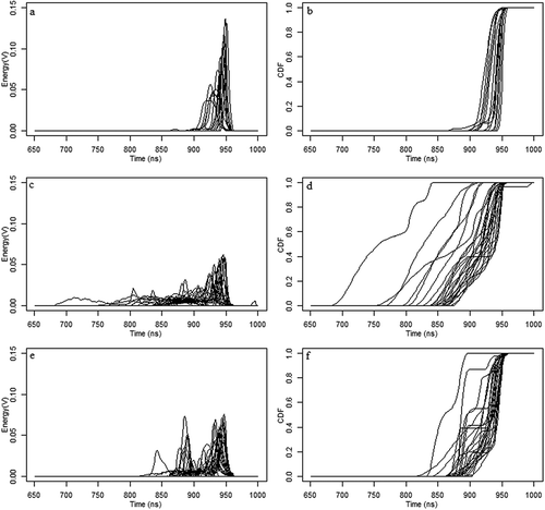
For the open space class, the within-class variation of the waveform curves is the smallest. The majority of waveforms for open space have similar single-echo shapes with late starting locations due to their low elevation and narrow echo widths because of their flat surface (Figure 3(a)). However, they differ slightly from each other in terms of the starting and ending location, the echo width, or the peak amplitude because of differences in surface elevation, slope, or material. The CDF curves of waveforms for open space generally exhibit a late rising location (where the CDF value begins to rise) and a steeply increasing edge that quickly reaches 1, with minor differences in the rising locations and the slopes of the increasing edges (Figure 3(b)). These characteristics make the waveforms for open space highly distinguishable from those for buildings and trees.

The tree class is characterized by a large within-class variation in the original waveform curves (Figure 3(c)) as well as in their corresponding CDF curves (Figure 3(d)). The original waveform curves for trees vary markedly in terms of starting location, number of echoes, and/or width and peak amplitude for each echo. This results in differences in their corresponding CDFs in terms of the rising locations, the slopes of increasing edges, and/or the areas under the CDF curves. These differences are primarily determined by tree heights, tree crown shapes, and/or the net coverage of trees within the footprints. For example, waveforms over tall trees usually have earlier starting locations, while waveforms over short trees often have relatively later starting locations, which contributes to the different rising locations in their corresponding CDF curves. Waveforms with a footprint containing multiple trees with bigger tree crowns usually have several wider echoes at high altitude, while waveforms with footprint covering trees with smaller tree crowns have several narrower echoes. Trees usually have gradually rising edges with varied degrees of slopes in their CDF curves. Overall, waveforms and their CDFs for the tree class have the highest within-class variation among the three classes. This makes it difficult to separate them visually from the waveforms in the other classes.

For the building class, Figure 3(e,f) shows moderate within-class variation, primarily due to the different types of buildings from which the waveforms were returned. There are three major types of buildings in the study area: flat-roofed, slope-roofed, and buildings surrounded by trees. Waveforms over flat-roofed buildings usually have two individual narrow echoes separated by a distance of a few meters to about 15 m. The top echo corresponds to the flat roof of the building, the bottom one corresponds to the flat ground, and the vertical interval between the two corresponds to the height of the building. Jointly, this generates a stair-step pattern (i.e. steep–flat–steep–flat) in their corresponding CDF curves, which makes it easy to separate waveforms over flat-roofed buildings from those over trees. Waveforms over slope-roofed buildings present different waveform patterns compared with those over flat-roofed buildings. Slope-roofed buildings generally have one wider echo resulting from scattering caused by the sloping roof. Consequently, the CDF curves of waveforms over slope-roofed buildings show a gradual–flat–steep–flat pattern, which are again clearly different from those over trees. However, for the buildings closely surrounded by trees, the waveform curves and their corresponding CDF curves exhibit similar patterns to those over trees, which can cause confusion between the tree and the building classes.

5.2. Performance comparison of different curve matching approaches

The average total percentage accuracy of the classification results over the 15 trials of randomly selected reference waveforms, in ascending order, was: 70% for CAM, 75% for CRSSDA, 79% for KS, 85% for CCAM and CCRSSDA, and 87% for KL.

5.2.1. Comparison of waveform-curve-based approaches

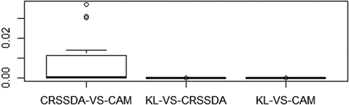
Among the three approaches that used the original waveform curve as inputs (CRSSDA, CAM, and KL), KL achieved the highest average classification accuracy in terms of total percentage accuracy. The results of McNemar’s chi-square test indicated that the performance of KL was significantly better than that of CAM and CRSSDA at a significance level of 0.0001 for all 15 trials (Figure 4). This result reconfirms the superiority of KL over HAM and HMRSSDA as in our previous study (Zhou and Qiu 2015). With respect to CRSSDA compared with CAM, Figure 4 shows that CRSSDA significantly outperformed CAM at a level of 0.01 for most of the 15 trials. This suggests that the performance of CRSSDA is in general significantly better or at least comparable to that of CAM.

Figure 4. Boxplot of the p-values of McNemar’s chi-square test among waveform-curve-based approaches across the 15 trials.

To achieve better insight, the within-class and between-class curve similarities measured by these three methods are shown in Figure 5 with all the measures normalized using RCDPB. The within-class curve similarities are obtained when the testing waveforms are from the same class as that of the reference waveforms. For example, if a testing waveform is from the building class, the within-class curve similarity for this testing waveform is the smallest RCDPB value between this testing waveform and all the reference waveforms in the building class, using a given method. After the within-class curve similarities for all the testing waveforms in the class are calculated for a given method, the boxplot of the within-class curve similarities (e.g. Building–Building) is then drawn. Similarly, the between-class curve similarities are obtained when the testing waveforms and the reference waveforms are from different classes. If a testing waveform is from the building class, the between-class curve similarity for this testing waveform to the tree class is the smallest RCDPB value between this testing waveform and all the reference waveforms in the tree class. Again, after the between-class curve similarities for all the testing waveforms in the class are calculated, the boxplot of the between-class curve similarities (e.g. Building–Tree) is produced.

Figure 5. Analysis of within-class and between-class curve similarity for the three waveform-curve-based approaches. For full colour versions of the figures in this paper, please see the online version.

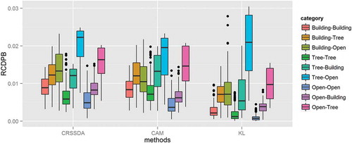
Figure 5 shows that CRSSDA, CAM, and KL differ considerably in the size of their interquartile boxes for the three within-class curve similarities (Building–Building, Tree–Tree, and Open–Open), the closeness of these boxes to the x axis, and the overlap of the boxes for within-class and between-class curve similarities. For KL, the boxes of the Building–Building, Tree–Tree, and Open–Open were much closer to the x axis and the ranges of their interquartile boxes were substantially smaller compared with those of CRSSDA and CAM. This explains why KL achieved the highest classification accuracy for all three classes. KL also had smaller overlaps of the boxes between the individual within-class and their corresponding between-class curve similarities than CRSSDA and CAM. Taking the building class as an example, there were smaller overlaps of the boxes between Building–Building and Building–Tree and between Building–Building and Building–Open for KL, while the corresponding overlaps of the boxes for CRSSDA and CAM were considerably larger. As a result, the probability that a testing waveform for the building class was misclassified as tree or open space when using KL was much lower than using CRSSDA and CAM.

In general, CRSSDA had similar patterns in their interquartile boxes to CAM in terms of their closeness to the x axis and ranges of the boxes for all the three within-class curve similarities. However, compared with CAM, CRSSDA had smaller overlaps of the boxes between the within-class and their corresponding between-class curve similarities for all the classes. Taking the open space class as an example, CRSSDA had a smaller overlap of the boxes between the within-class (Open–Open) and the between-class curve similarities (Open–Building) than CAM, even though the range of its box for the Open–Open within-class curve similarities was slightly larger than that of CAM. As a consequence, the probability of a testing sample of open space being misclassified when using CRSSDA was lower than using CAM.

5.2.2. Comparison of CDF-curve-based approaches

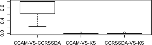
CCRSSDA, CCAM, and KS are all based on the CDF curves of the original waveforms. CCRSSDA and CCAM had similar performance, while KS performed slightly worse in terms of the average total percentage accuracy. The results of McNemar’s chi-square test indicated that there were no significant differences between the performance of CCRSSDA and CCAM and both performed significantly better than KS at the level of 0.05 (Figure 6). This is probably due to the fact that KS measures a single maximum absolute difference between two CDFs, while CCAM sums the angle differences and CCRSSDA sums the area differences of all the time bins between two CDFs.

Figure 6. Boxplot of the p-values of McNemar’s chi-square test among CDF-curve-based approaches across the 15 trials.

The within-class and between-class curve similarities measured by the three CDF-based methods are shown in Figure 7. As with the waveform-based curves, the measures were normalized using RCDPB. CCRSSDA and CCAM had similar patterns in the interquartile boxes in terms of their closeness to the x axis and the ranges of the within-class similarity boxes for all three categories. Similarly, both approaches had no major differences in the overlaps of the boxes between the within-class and the corresponding between-class curve similarities. These were consistent with the results of the McNemar’s test which showed no significant differences in performance between CCRSSDA and CCAM for all 15 trials.

Figure 7. Analysis of within-class and between-class curve similarity for the three CDF-curve-based approaches. For full colour versions of the figures in this paper, please see the online version.

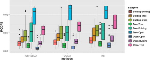
Compared with CCRSSDA and CCAM, KS had larger ranges of the boxes for the three within-class curve similarities and these boxes were farther away from the x axis. For the building class, KS had a larger overlap of the boxes between the within-class (Building–Building) and the between-class (Building–Tree) curve similarities. Consequently, the probability of a testing waveform in this class being misclassified as tree using KS was higher than using CCRSSDA and CCAM. For the tree and the open space classes, there were no overlaps of the boxes between the within-class and their corresponding between-class curve similarities for all three methods. However, compared with CCRSSDA and CCAM, KS had more extreme values above the within-class interquartile boxes that overlapped with the corresponding between-class interquartile boxes. This indicated that KS may not perform as well as CCRSSDA and CCAM for these two classes.

5.2.3. Comparison of waveform-curve-based and CDF-curve-based approaches

As mentioned above, CRSSDA, CAM and KL are based on the original waveform curves, while CCRSSDA, CCAM, and KS are based on their derived CDFs. Figure 8 shows boxplots of the results of the pairwise McNemar’s test between the three waveform-curve-based approaches and the three CDF-curve-based approaches for all 15 trials.

Figure 8. Boxplot of the p-values of McNemar’s chi-square test among waveform-curve-based and CDF-curve-based approaches across 15 trials.

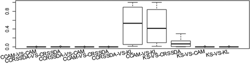
To assess the role of curve type (noncumulative versus cumulative), we specifically compared the performance of CRSSDA versus CCRSSDA and CAM versus CCAM. CRSSDA and CCRSSDA use the same root sum squared differential area-based algorithm and CAM and CCAM use the same angle mapper-based algorithm. With the CDF curves of waveform data as inputs, CCRSSDA and CCAM approaches achieved significant improvements at the level of 0.001 in classification accuracy compared with their noncumulative counterparts (Figure 8). For example, CCAM improved over CAM in average total accuracy by 15%. Regarding the within-class and between-class curve similarities (Figures 5 and 7), the within-class interquartile boxes for CCRSSDA and CCAM had smaller ranges and were much closer to the x axis for all three classes compared with CRSSDA and CAM, respectively. CCRSSDA and CCAM also had smaller overlaps between the within-class boxes and their corresponding between-class boxes for each class. Taking the building class as an example, CCRSSDA and CCAM had considerably smaller overlaps of the boxes between Building–Building and Building–Tree and between Building–Building and Building–Open compared with CRSSDA and CAM, respectively. This resulted in fewer building waveforms misclassified as trees or as open space. For a specific class, waveforms usually have similar patterns in their shapes, but may differ from each other in the local peaks and troughs, as well as the peak location and the width of each echo. CRSSDA and CAM are very sensitive to these differences, which causes these two approaches to perform relatively poorly. However, as Zhou et al. (2015) noted, the aggregation process inherent in creating CDFs tends to minimize these differences by cancelling the local peaks and troughs, thus their corresponding CDFs are more similar to each other in shape. As a consequence, the two CDF-curve-based approaches are preferable to their waveform-curve-based counterparts when the same algorithm is used for classification.

However, the CDF-curve-based approaches do not always perform better than the waveform-curve-based approaches when different algorithms are adopted. For example, KL is based on the original waveform curves, while KS is based on the CDF curves of the waveform data. KL performed significantly better than KS at the level of 0.005 for all 15 trials (Figure 8). For KL, its three within-class interquartile boxes had much smaller ranges and were closer to the x axis compared with those of KS (Figures 5 and 7). For the building class, KL did not have any overlap between the within-class and between-class interquartile boxes, while KS had a large overlap between within-class Building–Building and between-class Building–Tree. For the tree and open space classes, the within-class and between-class boxes for both KL and KS did not overlap, but KL had fewer extreme values above the within-class boxes that overlapped the between-class boxes than did KS.

Additionally, KL also achieved slightly higher average performance than CCRSSDA and CCAM, but these differences were not statistically significant at the 0.05 level (Figure 8). Finally, KS performed better or at least comparable with CRSSDA, and significantly better than CAM at the 0.005 level (Figure 8).

6. Conclusions

ICESat waveform data have been widely used for forest and urban studies by numerous researchers. Recently several studies have been conducted on ICESat waveform-based classifications. These studies were primarily based on waveform discretization and metrics derivation. In this study, we developed two groups of curve matching approaches that utilized the complete information provided by waveforms. As a case study, these approaches were applied to ICESat waveform data and were demonstrated to be effective in differentiating different classes in an urban environment. However, the set of curve matching approaches developed in this study could also be useful to process other LiDAR waveform data, including those acquired by airborne sensors with continuous coverage. To the best of our knowledge, besides our previous study (Zhou et al. 2015), we have not seen any research using complete waveform curve for land cover classification, which makes our study novel.

The shapes of the waveforms over different classes, such as tree, building, and open space, are primarily influenced by their vertical and horizontal composition within the waveform footprints. There exist considerable within-class variations due to different height levels, vertical structures, and footprint net coverage for each class. To reduce the impact of this high within-class variability on classification accuracy, multiple reference waveforms were selected by using random selection. A performance comparison of six curve matching approaches showed that KL provided the highest average classification accuracy, which was closely followed by CCRSSDA and CCAM, but there were no significant differences between any two of these methods. However, they all significantly outperformed KS, CRSSDA, and CAM. Another original finding in this study was that the two approaches based on the CDF-curve of waveforms are preferred over those based on the original waveform curves when the same algorithm is used for waveform classification. However, the CDF-curve-based approaches are not always superior to those based on original waveform curves when different algorithms are used. Future research is needed to assess if these CDF-curve-based approaches used for waveform classification would also achieve superior results when applied to pixel-based hyperspectral curves and object-based image histogram.

The use of ICESat waveforms alone for land use classification is unlikely a common practice due to the large spacing between its footprints and the presence of mixed land covers within its footprints. The primary goal of this research was to verify that the novel curve matching approaches developed in this research are able to capture vertical structure information of full waveforms for land-cover classification. The approach is likely appropriate for feature extraction from small footprint waveforms. With more and more airborne LiDAR systems now providing full waveforms with small footprints and contiguous coverage, curve matching approaches will play a more important role in complementing existing approaches to feature extraction and land cover classification. When combined with traditional remotely sensed imagery, LiDAR waveforms are expected to enhance the accuracy of traditional classification that relies on only 2D spectral information (Zhou and Qiu 2015).

However, the findings in this study may only apply to relatively flat areas similar to this study, since ICESat waveforms are sensitive to underlying terrain variation within the large footprints (Hilbert and Schmullius 2012). Future study may focus on removing the terrain effects from the ICESat waveforms in advance and then evaluate the performance of the six curve matching-based approaches to waveform-based classification over different types of terrain. In addition to the terrain effect, due to limitation of large footprint size of ICESat waveform data, waveforms with a mixture of several types with none exceeding 50% in coverage were excluded from this study. Classification of mixed ICESat footprints should be investigated using a fuzzy classification algorithm in the future. It is also important to point out that, if our proposed curve matching methods are applied to small footprint airborne LiDAR by segmenting the point clouds or the image into objects first and then synthesizing object-level pseudo-waveform using a histogram of discrete LiDAR returns or waveforms (Zhou and Qiu 2015), the mixed footprint problem would not be an issue anymore because each segment would have a dominant land cover type as a result of the segmentation process.

Acknowledgments

The authors would like to thank the National Snow and Ice Data Center by distributing ICESat data.

Disclosure statement

No potential conflict of interest was reported by the authors.

References

- Agresti, A. 1996. An Introduction to Categorical Data Analysis. New York: Wiley.
- Alexander, C., K. Tansey, J. Kaduk, D. Holland, and N. J. Tate. 2010. “Backscatter Coefficient as an Attribute for the Classification of Full-Waveform Airborne Laser Scanning Data in Urban Areas.” ISPRS Journal of Photogrammetry and Remote Sensing 65 (5): 423–432. doi:10.1016/j.isprsjprs.2010.05.002.
- Burt, J. and G. Barber. 1996. Elementary Statistics for Geographers. New York: The Guildford Press.
- Chang, C.-I. 2000. “An Information-Theoretic Approach to Spectral Variability, Similarity, and Discrimination for Hyperspectral Image Analysis.” IEEE Transactions on Information Theory 46 (5): 1927–1932. doi:10.1109/18.857802.
- Cheng, F., C. Wang, J. Wang, F. Tang, and X. Xi. 2011. “Trend Analysis of Building Height and Total Floor Space in Beijing, China Using ICESAT/GLAS Data.” International Journal of Remote Sensing 32 (23): 8823–8835. doi:10.1080/01431161.2010.547531.
- Cho, M. A., P. Debba, R. Mathieu, L. Naidoo, J. Van Aardt, and G. P. Asner. 2010. “Improving Discrimination of Savanna Tree Species through a Multiple-Endmember Spectral Angle Mapper Approach: Canopy-Level Analysis.” IEEE Transactions on Geoscience and Remote Sensing 48 (11): 4133–4142. doi:10.1109/TGRS.2010.2058579.
- Duong, H., R. Lindenbergh, N. Pfeifer, and G. Vosselman. 2009. “ICESat Full-Waveform Altimetry Compared to Airborne Laser Scanning Altimetry over the Netherlands.” IEEE Transactions on Geoscience and Remote Sensing 47 (10): 3365–3378. doi:10.1109/TGRS.2009.2021468.
- Farid, A., D. C. Goodrich, R. Bryant, and S. Sorooshian. 2008. “Using Airborne Lidar to Predict Leaf Area Index in Cottonwood Trees and Refine Riparian Water-Use Estimates.” Journal of Arid Environments 72 (1): 1–15. doi:10.1016/j.jaridenv.2007.04.010.
- Ghiyamat, A., H. Z. M. Shafri, G. A. Mahdiraji, A. R. M. Shariff, and S. Mansor. 2013. “Hyperspectral Discrimination of Tree Species with Different Classifications Using Single- and Multiple-Endmember.” International Journal of Applied Earth Observation and Geoinformation 23 (1): 177–191. doi:10.1016/j.jag.2013.01.004.
- Gong, P., Z. Li, H. Huang, G. Sun, and L. Wang. 2011. “ICESat GLAS Data for Urban Environment Monitoring.” IEEE Transactions on Geoscience and Remote Sensing 49 (3): 1158–1172. doi:10.1109/TGRS.2010.2070514.
- Guo, L., N. Chehata, C. Mallet, and S. Boukir. 2011. “Relevance of Airborne Lidar and Multispectral Image Data for Urban Scene Classification Using Random Forests.” ISPRS Journal of Photogrammetry and Remote Sensing 66 (1): 56–66. doi:10.1016/j.isprsjprs.2010.08.007.
- Hamada, Y., D. A. Stow, L. L. Coulter, J. C. Jafolla, and L. W. Hendricks. 2007. “Detecting Tamarisk Species (Tamarix spp.) in Riparian Habitats of Southern California Using High Spatial Resolution Hyperspectral Imagery.” Remote Sensing of Environment 109 (2): 237–248. doi:10.1016/j.rse.2007.01.003.
- Harding, D. J., and C. C. Carabajal. 2005. “ICESat Waveform Measurements of Within-Footprint Topographic Relief and Vegetation Vertical Structure.” Geophysical Research Letters 32 (21): 1–4. doi:10.1029/2005GL023471.
- Hilbert, C., and C. Schmullius. 2012. “Influence of Surface Topography on ICESat/GLAS Forest Height Estimation and Waveform Shape.” Remote Sensing 4 (12): 2210–2235. doi:10.3390/rs4082210.
- Jensen, J. R. 2004. Introductory Digital Image Processing: A Remote Sensing Perspective. 3rd ed. Upper Saddle River, NJ: Prentice Hall.
- Kruse, F. A., A. B. Lefkoff, J. W. Boardman, K. B. Heidebrecht, A. T. Shapiro, P. J. Barloon, and A. F. H. Goetz. 1993. “The Spectral Image Processing System (SIPS)-Interactive Visualization and Analysis of Imaging Spectrometer Data.” Remote Sensing of Environment 44 (2–3): 145–163. doi:10.1016/0034-4257(93)90013-N.
- Kullback, S., and R. Leibler. 1951. “On Information and Sufficiency.” The Annals of Mathematical Statistics 22 (1): 79–86. doi:10.1214/aoms/1177729694.
- Lee, S., W. Ni-Meister, W. Yang, and Q. Chen. 2011. “Physically Based Vertical Vegetation Structure Retrieval from ICESat Data: Validation Using LVIS in White Mountain National Forest, New Hampshire, USA.” Remote Sensing of Environment 115 (11): 2776–2785. doi:10.1016/j.rse.2010.08.026.
- Lefsky, M. A., M. Keller, Y. Pang, P. B. De Camargo, and M. O. Hunter. 2007. “Revised Method for Forest Canopy Height Estimation from Geoscience Laser Altimeter System Waveforms.” Journal of Applied Remote Sensing 1 (1). doi:10.1117/1.2795724.
- Mallet, C., and F. Bretar. 2009. “Full-Waveform Topographic Lidar: State-of-the-Art.” ISPRS Journal of Photogrammetry and Remote Sensing 64 (1): 1–16. doi:10.1016/j.isprsjprs.2008.09.007.
- Mallet, C., F. Bretar, M. Roux, U. Soergel, and C. Heipke. 2011. “Relevance Assessment of Full-Waveform Lidar Data for Urban Area Classification.” ISPRS Journal of Photogrammetry and Remote Sensing 66 (6): S71–S84. doi:10.1016/j.isprsjprs.2011.09.008.
- Molijn, R. A., R. C. Lindenbergh, and B. C. Gunter. 2011. “ICESat Laser Full Waveform Analysis for the Classification of Land Cover Types over the Cryosphere.” International Journal of Remote Sensing 32 (23): 8799–8822. doi:10.1080/01431161.2010.547532.
- Muss, J. D., D. J. Mladenoff, and P. A. Townsend. 2011. “A Pseudo-Waveform Technique to Assess Forest Structure Using Discrete Lidar Data.” Remote Sensing of Environment 115 (3): 824–835. doi:10.1016/j.rse.2010.11.008.
- Olszewski, D. 2012. “A Probabilistic Approach to Fraud Detection in Telecommunications.” Knowledge-Based Systems 26: 246–258. doi:10.1016/j.knosys.2011.08.018.
- Pirotti, F. 2010. “IceSAT/GLAS Waveform Signal Processing for Ground Cover Classification: State of the Art.” Italian Journal of Remote Sensing/Rivista Italiana di Telerilevamento 42 (2): 13–26. doi:10.5721/ItJRS20104222.
- Reitberger, J., C. Schnörr, P. Krzystek, and U. Stilla. 2009. “3D Segmentation of Single Trees Exploiting Full Waveform LIDAR Data.” ISPRS Journal of Photogrammetry and Remote Sensing 64 (6): 561–574. doi:10.1016/j.isprsjprs.2009.04.002.
- Rutzinger, M., B. Höfle, M. Hollaus, and N. Pfeifer. 2008. “Object-Based Point Cloud Analysis of Full-Waveform Airborne Laser Scanning Data for Urban Vegetation Classification.” Sensors 8 (8): 4505–4528. doi:10.3390/s8084505.
- Sasaki, T., J. Imanishi, K. Ioki, Y. Morimoto, and K. Kitada. 2012. “Object-Based Classification of Land Cover and Tree Species by Integrating Airborne Lidar and High Spatial Resolution Imagery Data.” Landscape and Ecological Engineering 8 (2): 157–171. doi:10.1007/s11355-011-0158-z.
- Sridharan, H., and F. Qiu. 2013. “Developing an Object-Based Hyperspatial Image Classifier with a Case Study Using Worldview-2 Data.” Photogrammetric Engineering & Remote Sensing 79 (11): 1027–1036. doi:10.14358/PERS.79.11.1027.
- Stow, D. A., S. I. Toure, C. D. Lippitt, C. L. Lippitt, and C.-R. Lee. 2012. “Frequency Distribution Signatures and Classification of Within-Object Pixels.” International Journal of Applied Earth Observation and Geoinformation 15 (1): 49–56. doi:10.1016/j.jag.2011.06.003.
- Sun, G., K. J. Ranson, D. S. Kimes, J. B. Blair, and K. Kovacs. 2008. “Forest Vertical Structure from GLAS: An Evaluation Using LVIS and SRTM Data.” Remote Sensing of Environment 112 (1): 107–117. doi:10.1016/j.rse.2006.09.036.
- Toure, S. I., D. A. Stow, J. R. Weeks, and S. Kumar. 2013. “Histogram Curve Matching Approaches for Object-Based Image Classification of Land Cover and Land Use.” Photogrammetric Engineering & Remote Sensing 79 (5): 433–440. doi:10.14358/PERS.79.5.433.
- Ussyshkin, V., and L. Theriault. 2011. “Airborne Lidar: Advances in Discrete Return Technology for 3D Vegetation Mapping.” Remote Sensing 3 (12): 416–434. doi:10.3390/rs3030416.
- Wagner, W., M. Hollaus, C. Briese, and V. Ducic. 2008. “3D Vegetation Mapping Using Small-Footprint Full-Waveform Airborne Laser Scanners.” International Journal of Remote Sensing 29 (5): 1433–1452. doi:10.1080/01431160701736398.
- Wang, X., X. Cheng, Z. Li, H. Huang, Z. Niu, X. Li, and P. Gong. 2012. “Lake Water Footprint Identification from Time-Series ICESat/GLAS Data.” IEEE Geoscience and Remote Sensing Letters 9 (3): 333–337. doi:10.1109/LGRS.2011.2167495.
- Zaletnyik, P., S. Laky, and C. Toth. 2010. “LIDAR Waveform Classification using Self-Organizing Map.” American Society for Photogrammetry and Remote Sensing Annual Conference, San Diego, USA, April 26–30.
- Zhou, W. 2013. “An Object-Based Approach for Urban Land Cover Classification: Integrating Lidar Height and Intensity Data.” IEEE Geoscience and Remote Sensing Letters 10 (4): 928–931. doi:10.1109/LGRS.2013.2251453.
- Zhou, Y., and F. Qiu. 2015. “Fusion of High Spatial Resolution Worldview-2 Imagery and Lidar Pseudo-Waveform for Object-Based Image Analysis.” ISPRS Journal of Photogrammetry and Remote Sensing 101: 221–232. doi:10.1016/j.isprsjprs.2014.12.013.
- Zhou, Y., F. Qiu, A. A. Al-Dosari, and M. S. Alfarhan. 2015. “IceSat Waveform-Based Land-Cover Classification Using a Curve Matching Approach.” International Journal of Remote Sensing 36 (1): 36–60. doi:10.1080/01431161.2014.990648.