Temporal replication of the national land cover database using active machine learning

Abstract

Regional and national level land cover datasets, such as the National Land Cover Database (NLCD) in the United States, have become an important resource in physical and social science research. Updates to the NLCD have been conducted every 5 years since 2001; however, the procedure for producing a new release is labor-intensive and time-consuming, taking 3 or 4 years to complete. Furthermore, in most countries very few, if any, such releases exist, and thus there is high demand for efficient production of land cover data at different points in time. In this paper, an active machine learning framework for temporal updating (or backcasting) of land cover data is proposed and tested for three study sites covered by the NLCD. The approach employs a maximum entropy classifier to extract information from one Landsat image using the NLCD, and then replicate the classification on a Landsat image for the same geographic extent from a different point in time to create land cover data of similar quality. Results show that this framework can effectively replicate the land cover database in the temporal domain with similar levels of overall and within class agreement when compared against high resolution reference land cover datasets. These results demonstrate that the land cover information encapsulated in the NLCD can effectively be extracted using solely Landsat imagery for replication purposes. The algorithm is fully automated and scalable for applications at landscape and regional scales for multiple points in time.

Keywords:

• active machine learning
• maximum entropy
• temporal replication
• National Land Cover Database (NLCD)
• information extraction

1. Introduction

Land cover data have taken an important role in geographic research where integration with other data sources allows for analyses at landscape, regional, and even global scales to carry out studies on topics ranging from urbanization (e.g., Galster et al. 2006; Shrestha et al. 2012) to landscape ecology (e.g., Driscoll et al. 2005; Montgomery et al. 2014). In order to assess changes in the landscape using land cover data, sufficient temporal coverage is necessary (e.g., Fall et al. 2010). Most regional or national land cover products are produced for only one or two points in time. Other products – such as the National Land Cover Database (NLCD) in the United States – cover extended time periods but are generally released at intervals between 5 and 10 years, which leaves researchers with an inhibitive, coarse temporal resolution. Furthermore, national level land cover datasets are expensive to produce and often take a number of years to complete. The above aspects illustrate an urgent need for land cover data for alternate points in time (to cover longer time periods), in particular where there are no national efforts on long-term land cover mapping in place, and at fine temporal resolution.

In principle, the fine temporal resolution and broad temporal extent of remote-sensing imagery – particularly from Landsat missions – allow for continuous monitoring of the Earth’s surface over extensive periods of time (e.g., the first Landsat was launched in 1972). However, while such imagery could potentially be used to produce annual land cover data, regional and national level classifications generally rely on significant amounts of ancillary data to achieve acceptable accuracy levels (e.g., Büttner and Kosztra 2007; Homer et al. 2007). Thus, the process of temporal updating of such land cover datasets, which is usually based on detecting areas that have changed since the previous release and reclassifying these areas (e.g., Fry et al. 2011; Jin et al. 2013), is labor-intensive, time-consuming, and data-demanding. In order to generate broad scale land cover data at finer temporal resolutions and of similar accuracy, this process needs to be streamlined and automated. The integration of ancillary data in the classification process encapsulates a rich knowledge base in the land cover data, which presents an opportunity for information extraction approaches. The research presented here aims to advance this field by establishing a formal methodological foundation for temporal replication of an existing land cover dataset using image cross-decomposition and active machine learning. Previous work conducted by the authors developed a methodology for spatial extrapolation of the NLCD (Maclaurin and Leyk 2016), which this paper builds upon and extends into the temporal domain. Replication of land cover data at different points in time presents a unique set of challenges including temporal differences in vegetation productivity (e.g., due to drought or disease), varying states of agricultural land (e.g., fallow, production, or harvested), and modifications to the built environment. The classifier must be able to distinguish between variability within certain land cover classes and conversion to a different class (i.e., land cover change). Thus, the training sample from the source image must be selected in a way that it can be used to effectively classify the target image (i.e., temporal domain adaptation).

A broad body of research has addressed domain adaptation for image classification in the spatial and temporal domains. Signature extension has been used in remote sensing to apply a supervised classification to a series of Landsat scenes (spanning either space or time) after extensive radiometric correction (Olthof, Butson, and Fraser 2005). Such an approach effectively extracts information from the classified scene and applies it to the series of imagery. However, the procedure is still highly dependent on an interpreter throughout the classification process and therefore cannot be fully automated. In the field of machine learning, methods for extracting information from source data to classify target data have been developed and broadly applied (Huang et al. 2010; Sebastiani 2002). However, machine learning methods have only recently been tested in similar ways for extending a land cover classification in the spatial or temporal domains. Alajlan et al. (2014) proposed an approach for improving the generalizability of training data to classify continental scale land cover data. Persello and Bruzzone (2012) developed a method to apply the training sample describing a land cover classification collected from a source image to classify a target image, i.e., to spatially extrapolate the training sample. In the temporal domain, Bruzzone and Marconcini (2009) proposed a domain adaptation support vector machine (SVM) approach that could potentially be used for temporal updating of land cover data. Using Landsat 5 Thematic Mapper (TM) imagery for a small study area, the authors used a training sample from one point in time to classify an image from a later point in time.

Overall, most of the relevant research has focused on theoretical approaches, making use of synthetic land cover data. Here we expand on this body of research in an applied context to replicate an existing land cover dataset – the NLCD – for a different point in time. We propose an active machine learning framework using a maximum entropy classifier to extract information from one Landsat image using the NLCD for one point in time to train the algorithm, and then reproduce the classification using a Landsat image from a different point in time. The approach rests on the central idea that information encapsulated in the NLCD – a rich knowledge base created through the incorporation of ancillary data sources and a labor-intensive classification procedure, as described earlier – can be extracted for temporal replication of the database. This would make it possible to automate the production of NLCD-comparable datasets for different points in time and would facilitate future updates to large scale land cover datasets.

2. Background

2.1. Partial least squares (PLS) cross-decomposition to improve bi-temporal image comparison

Cross-decomposition algorithms model the correlation structures between two matrices to produce an orthogonal transformation that minimizes the variation in each matrix that is not correlated to the other (Trygg and Wold 2002). Cross-decomposition is a variation of principal component analysis (PCA), which applies a joint transformation on two multivariate datasets. Canonical correlation analysis (CCA) and PLS implementations have been used widely in remote sensing to maximize comparability between two images. Nielsen (2002) demonstrated the efficacy of cross-decomposition for multi-temporal image analysis using Landsat TM data. Canty, Nielsen, and Schmidt (2004) developed a change detection algorithm – multivariate alteration detection (MAD) – based on a CCA cross-decomposition of bi-temporal images. Wolter et al. (2008) used PLS to determine the relationship between in situ sampled data and Landsat imagery.

PLS can be used to jointly decompose two sets of variables into maximally correlated pairs of transformed variables to ensure comparability for further modeling (Geladi 1988; Nielsen 2002). Specifically, in this study the canonical form of two block PLS (designated PLS-C2A) developed by Wold (1975) was applied, which models the cross-covariance of two matrices (Wegelin 2000). Two bi-temporal images, time₁ and time₂, are decomposed based on pairs of latent (or hidden) variables (ξ₁,ω₁), …, (ξ_i,ω_i) such that each pair is orthogonal. The latent variables are essentially pairs of coefficient vectors used to perform the joint image decomposition. This maximizes the covariance of the first pair of latent variables, Cov(ξ₁,ω₁). The subsequent pairs of latent variables are obtained iteratively such that the pairs of transformed components (of the time₁ and time₂ images) are mutually orthogonal and each pair is maximally correlated (Wegelin 2000). The PLS cross-decomposition produces an orthogonal space where the first few transformed components explain most of the shared variance between the time₁ and time₂ images. Given that the decomposed components are linear combinations of the bi-temporal image pair, PLS effectively reduces dimensionality and reduces noise in the original images (Nguyen and Rocke 2004).

2.2. Maximum entropy for modeling incomplete information

Maximum entropy (MaxEnt) models have been used extensively to work with incomplete information in machine learning (Berger, Pietra, and Pietra 1996) and in research with a geographic focus (Kapur 1989). MaxEnt has been applied broadly in ecology for modeling species distributions (Baldwin 2009; Phillips, Anderson, and Schapire 2006), and more recently it has been applied in demographic modeling (Leyk, Nagle, and Buttenfield 2013; Ruther et al. 2013). In remote sensing, maximum entropy models have been used in land cover classification with aerial photography (Li and Guo 2010) and Landsat TM imagery (Alexakis et al. 2012; Maclaurin and Leyk 2016), in multi-seasonal habitat mapping in Germany (Stenzel et al. 2014), and in country-level forest biomass mapping in Mexico (Rodríguez-Veiga et al. 2014). MaxEnt models are general-purpose statistical approaches based on the principle that predictions should be based on what is known while making no assumptions about what is unknown (Jaynes 1957). A MaxEnt model estimates the probability distribution for the outcome variable with maximum entropy (i.e., the most uniform) conditioned on a set of constraints, which represent the known information. In the context of land cover classification, MaxEnt estimates the conditional probability distribution p(y = c|x) that pixel y belongs to class c given the pixel vector values x from the finite set X of the underlying remote sensing data. While satisfying the constraints on p(y|x), derived from the training sample for class c, the estimated conditional distribution is as uniform as possible (Li and Guo 2010). MaxEnt is a general-purpose probability based classification method that can readily be applied in complex machine learning frameworks (e.g., Maclaurin and Leyk 2016), and thus represents a promising approach for the problem of temporal replication of land cover data.

2.3. Active machine learning for land cover classification

In the machine learning literature, active learning is a semi-supervised framework, which allows the classifier to compile the training sample following predefined criteria, rather than relying on manual selection or random sampling (Thompson, Califf, and Mooney 1999). This is generally an iterative procedure in which the classifier identifies the best candidates to add to a training sample S from a pool of potential training data based on a specified heuristic (Settles 2010). In such a framework, margin sampling is an effective heuristic which determines potential instances to be added to the training sample by selecting those that have the highest confusion among classes predicted by the classifier (e.g., the MaxEnt model) in the prior iteration. In margin sampling, the highest and second highest predicted class probabilities for each instance in the potential training data pool are differenced and instances with the lowest differences (i.e., highest confusion) are candidates to add to S (Scheffer, Decomain, and Wrobel 2001). The margin sampling heuristic within an active learning framework allows the classifier to effectively separate classes by labeling and adding instances along class boundaries and thus helps the classifier resolve ambiguous cases in the next iteration. This approach rests on the assumption that labeling high confusion instances will help distinguish between classes better than labeling instances with the lowest confusion (i.e., the most pure examples from each class). Research in natural language processing and in remote sensing has demonstrated the strength of an approach based on this assumption (Foody and Mathur 2006; Juszczak and Duin 2003).

Traditionally, active learning has been used mainly in computer vision and natural language processing (Settles 2010). Only recently has active learning been applied in remote sensing image classification. Approaches have been developed to improve land cover classification (Tuia et al. 2009) and to address the problem of domain adaptation between source and target data (Maclaurin and Leyk 2016; Persello and Bruzzone 2012; Persello 2013). Tuia, Pasolli, and Emery (2011) used active learning and a clustering-based strategy to discover classes that were not represented in the training area. Active learning has also been used for semi-supervised image segmentation in hyperspectral imagery (Li, Bioucas-Dias, and Plaza 2010). This growing area of research on active learning frameworks within the remote sensing community has shown promising results (Crawford, Tuia, and Yang 2013). For this reason, the methodology described here expands on this body of work by implementing margin sampling within an active learning maximum entropy framework for temporal replication of existing land cover data using only remote-sensing imagery.

2.4. The national land cover database

Developed by the United States Geological Survey (USGS), the NLCD represents the highest quality land cover data at 30 m resolution available for the conterminous U.S. released for multiple points in time starting in 1992. The database has been applied extensively in research ranging from demographic modeling (e.g., Chi 2010; Leyk et al. 2014) to wildlife conservation and landscape ecology (e.g., Driscoll et al. 2005; Montgomery et al. 2014). NLCD classes are based on the Anderson land classification scheme (Anderson 1976), which is a hierarchical system for categorizing land cover types. General categories (level I), such as developed land or forest, are further divided into more specific (level II) classes, e.g., developed land is broken down into four level II classes: open space developed, and low, medium, and high intensity developed land (Homer et al. 2004). In this paper, we focus on temporally replicating the NLCD for level I classes. The NLCD 2001 was based on a decision tree classification framework using Landsat 5 TM and Landsat 7 ETM+ imagery and a number of ancillary datasets (Homer et al. 2004). The underlying Landsat imagery represented three periods in the phenological cycle to capture seasonal differences: spring, leaf-on, and leaf-off. Spatial clusters were created from the input images using decision trees and then ancillary data and high resolution aerial photography were used to place the clusters into meaningful classes (Homer et al. 2007). In a post-processing step, roads from U.S. Census TIGER files were burned in to the NLCD and classified as developed (level I) and open space developed (level II) land.

Since the 2001 release, subsequent versions for 2006 and 2011 have been produced; these three releases are the focus in this study. These releases are updates based on detecting change and reclassification of change pixels (Fry et al. 2011; Jin et al. 2013). While the database is released at 30 m resolution, the USGS recommends that it not be used at local scales (Homer et al. 2007), as accuracy levels do not support such analyses. The USGS conducted a validation on the 2001 and 2006 releases, showing level I accuracies of 85% and 84%, respectively (Wickham et al. 2010, 2013). Assessment of the NLCD 2011 had not been conducted at the time of writing. Independent research has documented limitations of the database in specific applications (e.g., Smith et al. 2010; Thogmartin et al. 2004; Wardlow and Egbert 2003). Hollister et al. (2004) identified scale dependence in an accuracy assessment of the database, with accuracy increasing when assessed on larger geographic extents. Furthermore, the assessment of the NLCD 2001 conducted by the USGS found significant regional variation ranging from 71% to 91% for level I classification accuracy (Wickham et al. 2010). Producer’s and user’s accuracies for the NLCD 2001 varied from as low as 19% to over 99% (Wickham et al. 2010). Given this body of research, significant regional variation, across-class variation, and scale dependence in NLCD accuracy should be expected. These are relevant points in this study because the NLCD represents a land cover classification with considerable class-level variation and misclassification rates. As a natural consequence, a replication framework that is trained on such imperfect databases will likely show some expected behavior. First, the classification accuracy of the replicated data may be similar but depending on inherent NLCD-class variability can also deviate from NLCD class accuracies. Furthermore, it cannot be expected that the replicated data will show considerable improvement over NLCD, which this study is attempting to replicate. In other words, the inherent quality issues of the NLCD may be the reason why a replication framework will be unable to generate the exact same or improved data quality. However, this study is an attempt to explore these aspects.

3. Study areas, data, and preprocessing

Three study sites were selected to assess the replication algorithm under different landscape conditions and scenarios of change (Figure 1). Selection of study sites was based on the availability of high resolution land cover datasets used to assess the replication results. Mid-summer Landsat 5 TM surface reflectance corrected image pairs (Masek et al. 2006) were used for all three study sites. The years chosen for temporal replication were also based on (and constrained to) the year of production of each reference dataset, as explained in the following.

Figure 1. The NLCD is shown at Anderson level I for the three study areas. White regions in the Tompkins, NY (TMPKNS) site are masked out clouds; these areas were excluded from the analysis.

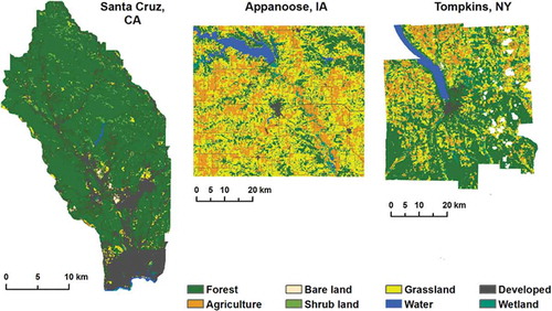
The first site covers the San Lorenzo river basin in Santa Cruz County, California. The river basin is dominated by forest with the city of Santa Cruz occupying the southern part of the study area. The site covers an area of 387 square km. Over the study period from 2001 to 2011, the river basin had a decrease in forested and agricultural area and an increase in developed and shrub land. However, the study period was reversed (i.e., the opposite direction was used for replication over time) because the reference dataset is from 2001; this provides an example of projecting backwards in time with the algorithm and thus an interesting experiment regarding its flexibility, i.e., 2011 was used as time₁ and 2001 was time₂. The Landsat scenes used for this site were captured on 5 August 2001 and 1 August 2011. The reference dataset was the 2001 high resolution Coastal Change Analysis Program (C-CAP) land cover dataset, which was produced from 4 m Quickbird imagery using an object based classification method. No formal assessment of the dataset has been conducted; however, it was reviewed extensively by NOAA analysts for logical and positional consistency using high resolution aerial photography (NOAA, 2008). The dataset was reclassified to match the NLCD level I classes and then resampled to 30 m resolution using a majority rule.

The second site covers Appanoose County, Iowa (1339 square km), which is a heterogeneous landscape dominated by grassland and agriculture, with some forest, shrub land, and a small presence of developed area. The study period is from 2001 to 2011, during which the county saw a decrease in forest, shrub, grassland, and water and an increase in agriculture and developed land. Landsat scenes were from 7 August 2001 and 4 September 2011. Time₂ was selected as 2011 to coincide as close as possible to the reference dataset, which was developed by the Iowa Department of Natural Resources for 2009, based on one meter resolution multispectral aerial photography from the National Agricultural Imagery Program (NAIP). An initial ISODATA unsupervised classification resulted in 250 classes, which were later refined with a supervised maximum likelihood classifier into 15 final classes. While completeness and logical consistency were ensured, formal accuracy assessment has not been conducted (Iowa DNR, 2012). We reclassified the dataset to match the NLCD level I classes and resampled it to 30 m resolution based on a majority rule.

Tompkins County, New York is the third study site, which covers 1257 square km. The city of Ithaca is the county seat and the surrounding area is forested with significant amounts of cropland and grassland. Tompkins County presents a rather heterogeneous landscape, similar to the APPNS site. The Tompkins study period was shorter because reference data were only available for 2007. During the study period from 2001 to 2006 the county saw a decrease in forest, shrub and grassland and an increase in agriculture and developed land. The Landsat scenes used for this site were captured on 7 June 2001 and 5 June 2006. The reference dataset from 2007 was produced by the Tompkins County Planning Department (TCPD) by manual interpretation of vector land cover polygons from color digital ortho-imagery and ancillary data from wetland, hydrology, parcel, and planning data (TCPD, 2009). Classes were reclassified to match level I of the NLCD and then polygons were converted to a raster dataset with 30 m resolution.

Semantic differences between the NLCD and the reference land cover datasets likely exist and this was an additional reason for applying the proposed framework on the Anderson level 1 classes. The definition of evergreen forest, for example, varied slightly between the CCAP and the NLCD. The CCAP classification defined evergreen forest as areas with more than 67% of trees that do not drop their leaves seasonally. The NLCD uses a similar definition with a threshold of more than 75%. Aggregating to Anderson level 1 classes (e.g., combining all forest classes) reduces the semantic differences between the NLCD and the reference datasets.

4. Methods

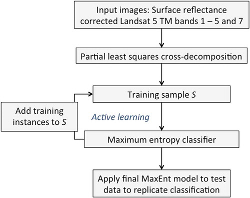
The information extraction algorithm for extending the NLCD in the temporal domain is described in this section (Figure 2). In Section 4.1, an approach is described to reduce residual differences (after atmospheric correction) between pairs of Landsat images (time₁ and time₂) in each study area, which maximizes comparability and thus applicability of the classification framework to the image pair. Section 4.2 explains the maximum entropy model used as the classifier in the active learning framework. A method for excluding likely misclassified NLCD pixels from the training sample collected from the time₁ image is then described in Section 4.3. Section 4.4 describes the components of the active learning routine applied to classify the image from time₂.

Figure 2. Flowchart of methods.

4.1. Improving image comparability through PLS cross-decomposition

Surface reflectance corrected Landsat image pairs were used for all three sites to minimize artifacts introduced by atmospheric and illumination conditions and sensor viewing geometry. While this correction significantly improves comparability for bi-temporal image analysis (Masek et al. 2006), residual variation from these sources can still persist between the two images. Environmental, on-the-ground variation – such as differences in productivity of vegetation or varying states of agricultural land – can further impair effective extraction of information from the image at time₁ used subsequently for replication at time₂. A PLS cross-decomposition was, therefore, applied to the Landsat image pairs for each study area to reduce residual differences attributable to the remote sensor and environmental variation. Similar to a PCA transformation, except applied jointly to two multispectral images, PLS captures the majority of the correlated variability between images in the first few transformed components and isolates the uncorrelated variability between the two images to the last components (Nielsen 2002; Wegelin 2000). PLS cross-decomposition, therefore, had two benefits: bi-temporal image pairs were transformed into maximally correlated component pairs and the dimensionality (i.e., the number of transformed bands) was reduced (Nguyen and Rocke 2004). For each study site, the PLS was applied to the image pair and the first three components in the transformed space were used to further refine the training sample in the procedure described in Section 4.3.

4.2. Maximum entropy model for information extraction

The training sample consisted of pixel vectors from the time₁ cross-decomposed image (Section 4.1) paired with the corresponding NLCD labels from time₁. Starting with the most uniform distribution (i.e., all values had equal probability of occurrence), the unknown distribution was constrained by a set of real-valued functions (f₁, f₂,…, f_n), which were derived from the training sample (Li and Guo 2010). In this fitting procedure, the MaxEnt model has a tendency to overfit the distribution to the constraints, which can produce poor predictions. Regularization is a way of solving the MaxEnt model that avoids overfitting by minimizing a specified loss function and allowing the model to approximate the properties specified by the constraints (Dudík, Phillips, and Schapire 2007; Maclaurin and Leyk 2016). MaxEnt classification was implemented using the LIBLINEAR library (Fan et al. 2008), with L2 regularization to minimize the loss function for l training vectors as follows:

where y is the class label, the training vector x is from the cross-decomposed image, and w is a weights vector generated by the model (w^T indicates the transpose of w). The LIBLINEAR library implementation of MaxEnt can produce a multiclass classification from multiple one-vs.-rest classifiers by normalizing the conditional probabilities for k classes with the following heuristic:

where the training vector is x and w is the weights vector (Fan et al. 2008). MaxEnt was used in two different ways here: as a binary classifier to filter out likely misclassified pixels from the potential training data pool (Section 4.3) and in the multiclass active learning framework described in Section 4.4 to actually replicate the NLCD from time₁ to time₂.

4.3. Removing likely misclassified training pixels to improve learning capabilities

Since producer’s and user’s accuracies for individual NLCD 2001 classes vary from as low as 19.4% to over 99% in the NLCD validation regions in which the three study areas are located (Wickham et al. 2010), misclassified pixels were expected to limit the efficacy of the extraction algorithm. To address this, we implemented a simple approach to filter out pixels from each NLCD class that were likely misclassified and would thus impede the learning process. The following procedure was applied separately for each of the eight level I classes. The MaxEnt classifier was used to produce probability estimates for the decomposed time₁ image, trained on all time₁ NLCD pixels for class y. Then, a probability threshold was selected by maximizing agreement between pixels with probabilities above this threshold and the NLCD pixels for class y. Pixels above this threshold were selected from the time₁ image for each class to produce the time₁ training data. For example, all forest pixels from the time₁ NLCD were used to estimate probability membership to forest for each pixel in the time₁ image. Next, a probability threshold was iteratively increased from 0 to 1 in increments of 0.01. A threshold was selected that produced the highest agreement between the NLCD forest pixels and the pixels with a probability above the threshold. The pixels above this threshold formed the time₁ training data for the forest class. This filtering approach effectively removed likely misclassified pixels from the time₁ image training data and was intended to improve the learning process described in Section 4.4. The remaining time₁ pixels (i.e., the training data) and the time₂ image pixels (i.e., the test data) were combined into one matrix (referred to hereafter as the input image). This was done to train the MaxEnt model on the NLCD labels from the time1 image and then fit the model to the time₁ and time₂ data together, rather than fitting to time₁ and then using the model to predict probabilities for time₂. Research by Tuia, Pasolli, and Emery (2011) showed that fitting the machine learning model to both images improved the prediction results. In our initial tests, we also found that fitting the data together produced a more generalizable and reproducible model and improved predictions for time₂.

4.4. Active learning for temporal land cover data replication

The training sample S was initiated with 50 pixels randomly sampled for each class from the potential training data pool (i.e., from the time₁ portion) in the input image. The MaxEnt model was then fit to S, producing eight normalized probability surfaces (Section 4.2). Using the margin sampling heuristic, the highest and second highest probabilities were differenced for each pixel in the training data pool of the input image in order to identify pixels with the highest confusion among classes. For each class, P pixels with the smallest differences (highest confusion), given that one of the highest probabilities actually belonged to the class, were added to S. The number of pixels, P, was based on a weighting strategy to increase the sample size of poorly performing classes. This approach improved the classification of these classes because it provided additional examples of problematic pixels on which the MaxEnt model was trained. The algorithm was allowed to add a total of 400 pixels per iteration distributed among the eight classes (i.e., 50 pixels on average per class per iteration). Sensitivity to the total number of pixels added in each iteration was tested using 200, 400, 600, and 800 pixels, and 400 provided the best results based on the final overall agreement with the NLCD. The proportion of the 400 pixels allocated to each class for the next iteration was calculated as a function of each class’s performance in replicating the NLCD for the training portion of the input image in that iteration. The number of pixels P from class k added to S was

where the average commission and omission error (ACOE_k) (Liu, Frazier, and Kumar 2007) was calculated for class k by comparing the replicated land cover classification for that iteration to the time₁ NLCD. The PLS cross-decomposition (Section 4.1) and filtering of likely misclassified pixels (Section 4.3) improved the generalizability of the MaxEnt model from the source to the target pixels. Because of this, the ACOE was a good indicator of how well the model would replicate the NLCD for the test pixels, and thus an effective metric for the weighting strategy.

As described earlier, P_k pixels – for each class k – with the smallest probability differences were added to S and the algorithm continued to the next iteration. The weighting strategy improved classification results for low prevalence classes more effectively compared to a fixed number for P by increasing the sample size specifically for those classes. The active learning routine was repeated until the change in overall agreement between the classified training portion of the input image and the NLCD training labels fell below a specified threshold or a maximum number of iterations were reached, whichever occurred first. The change in overall agreement was calculated within a window of the previous 25 iterations to account for variation from iteration to iteration. For this experiment, the threshold change in overall agreement was set at 0.01% and a maximum of 1000 iterations were allowed.

5. Results

The NLCD at time₂ was compared against the reference dataset as a baseline for the assessment of the replicated land cover dataset (RLCD) produced here. The overall agreement (OA) between the time₂ NLCD and reference data was 77.6%, 52.5%, and 63.7% for the SNTCRZ, APPNS, and TMPKNS sites, respectively. The reader may be reminded that the objective of the proposed methodology was to replicate similar levels of agreement as the time₂ NLCD and thus produce data of similar quality for different points in time. Therefore, the more similar the NLCD-reference and RLCD-reference agreements are the more successful the temporal replication would be. Overall agreement between the RLCD and the reference data was 85.8%, 51.8%, and 43.5% for SNTCRZ, APPNS, and TMPKNS, respectively. Temporal replication showed slightly higher agreement over the time₂ NLCD for the SNTCRZ site, very similar agreement for the APPNS site, and lower agreement for the TMPKNS site. Comparing the OA between the NLCD and the RLCD showed similar levels of agreement as the NLCD and RLCD compared to the reference: 89.5%, 58.5%, and 47.2% for STNCRZ, APPNS, and TMPKNS, respectively (Table 1).

Table 1. Overall agreement (OA) for the RLCD and NLCD compared to the reference data, and the RLCD–NLCD OA for all pixels in each study area.

	OA all pixels			OA change pixels
Study site	NLCD-ref. (%)	RLCD-ref. (%)	RLCD–NLCD (%)	NLCD-ref. (%)	RLCD-ref. (%)	RLCD–NLCD (%)
SNTCRZ	77.6	85.8	89.5	33.3	56.6	59.5
APPNS	52.5	51.8	58.5	32.0	39.8	36.7
TMPKNS	63.7	43.5	47.2	41.8	36.9	36.3

OA is also shown for only change pixels between time₁ and time₂ based on the two NLCD releases.

As described in Section 2.3, the NLCD 2006 and 2011 were updates of the previous release, where change pixels were identified and then reclassified, and thus the updated NLCD versions were exactly the same as the previous release for non-change pixels. We therefore also assessed the NLCD at time₂ and RLCD for only the pixels that changed between two releases of the NLCD. Overall agreement compared to the reference datasets for the NLCD at time₂ were 33.3%, 32.0%, and 41.8% for the STNCRZ, APPNS, and TMPKNS sites, respectively. For the RLCD-reference, OA was 56.6%, 39.8%, and 36.9% for the three sites, respectively (Table 1), and thus achieved comparable results. The RLCD showed higher agreement in comparison to the time₂ NLCD for the SNTCRZ and APPNS sites, and agreement was slightly lower for the TMPKNS site.

Qualitatively, the RLCD replicated the major landscape characteristics well in all three study sites (Figures 3–5) when compared to the NLCD of time₂. The methodology effectively captured major urban areas, water bodies, and dominant landscape features (e.g., vegetation corridors, agricultural and grassland areas, etc.). Within class producer’s and user’s agreements between RLCD and reference were consistent with the time₂ NLCD-reference agreements for most classes (Table 2). Wetland in general was replicated poorly compared to the NLCD. Bare land was challenging in the APPNS and TMPKNS sites, though time₂ NLCD-reference agreement was quite low to start with. The developed class was replicated well for the SNTCRZ and APPNS sites, yet posed a challenge for the TMPKNS site. Producer’s agreement was lower for the APPNS and TMPKNS sites, yet user’s agreement was higher. For most classes in all three sites, producer’s and user’s agreements balanced performance of the RLCD compared to the time₂ NLCD.

Table 2. Producer’s (PA) and user’s (UA) agreement (as percentages) for the NLCD and RLCD compared to the reference datasets.

	SNTCRZ				APPNS				TMPKNS
	NLCD		RLCD		NLCD		RLCD		NLCD		RLCD
Class	PA	UA	PA	UA	PA	UA	PA	UA	PA	UA	PA	UA
Forest	83.4	93.1	94.3	92.8	66.2	40.5	40.2	47.1	85.2	85.4	48.0	91.8
	(80.2)	(71.9)	(80.2)	(81.5)	(12.5)	(21.4)	(13.9)	(11.9)	(44.5)	(44.4)	(45.7)	(23.9)
Agriculture	0.0	0.0	0.0	0.0	55.4	52.6	55.8	41.5	52.7	62.4	37.1	65.8
	(0.4)	(0.1)	(0.3)	(~0)	(21.1)	(22.2)	(21.1)	(28.4)	(16.5)	(13.9)	(16.2)	(9.1)
Bare land	34.6	76.0	21.1	82.2	0.2	16.9	0.0	0.0	0.8	1.2	0.0	0.0
	(0.6)	(0.3)	(0.6)	(0.1)	(2.9)	(0.1)	(5.9)	(~0)	(0.2)	(0.2)	(0.2)	(~0)
Shrub	22.4	49.3	23.4	38.5	1.8	17.6	1.0	15.4	15.1	22.9	17.5	11.6
	(6.4)	(2.9)	(6.4)	(3.9)	(11.2)	(1.1)	(11.2)	(0.7)	(8.9)	(5.9)	(8.9)	(13.5)
Grassland	30.7	52.1	41.3	43.6	65.8	61.5	73.2	56.6	62.1	31.2	89.8	25.4
	(3.4)	(2.0)	(3.4)	(3.2)	(42.0)	(45.0)	(42.3)	(54.6)	(12.0)	(23.9)	(12.1)	(42.6)
Water	66.9	91.1	66.2	97.1	74.7	91.6	66.0	99.8	87.7	97.5	61.2	99.8
	(0.6)	(0.5)	(0.6)	(0.4)	(4.9)	(4.0)	(4.9)	(3.3)	(3.5)	(3.2)	(3.6)	(2.2)
Developed	95.0	33.7	87.0	63.0	46.1	17.2	42.1	6.5	24.4	76.4	3.2	22.8
	(7.8)	(22.1)	(7.8)	(10.8)	(1.9)	(5.1)	(0.2)	(1.0)	(11.1)	(3.5)	(10.0)	(1.4)
Wetland	16.9	43.4	0.0	0.0	22.5	5.2	1.1	8.6	76.9	49.4	20.1	8.8
	(0.6)	(0.2)	(0.6)	(~0)	(0.5)	(2.0)	(0.5)	(0.1)	(3.2)	(5.0)	(3.2)	(7.3)

The percent of the total number of pixels corresponding to each PA or UA value from the confusion matrix is shown in parentheses. For example, the PA for forest in the SNTCRZ NLCD was 83.4%, and according to the reference dataset 80.2% of all pixels in the study area were forest. The forest UA for the NLCD was 93.1%, and 71.9% of all pixels in the SNTCRZ study were classified as forest (either correctly or incorrectly) by the NLCD.

Figure 3. The RLCD for 2001, NLCD 2001, and C-CAP reference dataset for the Santa Cruz site.

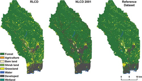
Figure 4. The RLCD for 2011, NLCD 2011, and Iowa DNR reference dataset for the Appanoose County, Iowa.

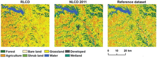
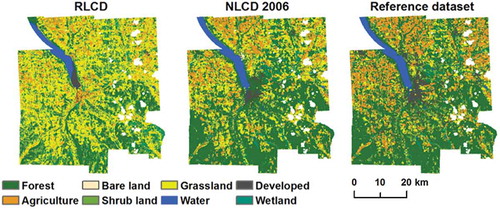
Figure 5. The RLCD for 2006, NLCD 2006, and TCPD reference dataset for Tompkins County, NY.

6. Discussion

Results show that the described approach for information extraction can effectively be used for temporal updating (and backcasting) of land cover data relying solely on remote-sensing imagery. Bi-temporal (surface reflectance converted) Landsat 5 TM images were cross-decomposed to reduce residual differences in illumination, atmospheric and environmental conditions between the two points in time. Then a filtering method was applied to remove likely misclassified time₁ NLCD pixels from the training data pool. The active learning MaxEnt classification routine produced levels of OA and within class producer’s and user’s agreement with the reference datasets similar to those of the time₂ NLCD. While the OA of the time₂ NLCD compared to the reference dataset was fairly high for the SNTCRZ site, it was surprisingly low for the APPNS and TMPKNS sites. The fact that the RLCD for each study area produced OA levels similar to the time₂ NLCD (when compared to the reference data) suggests that temporal updating of land cover data relies heavily on the quality of the original land cover data at time₁. The relatively low agreement between NLCD and RLCD could be a consequence of the low accuracy levels in NLCD classes and the difficulty of training machine learning algorithms on imperfect land cover data. However, as mentioned earlier, the outcome of similar NLCD-reference and RLCD-reference agreements is actually a desired feature of the extraction methodology because the underlying goal was equivalent and comparable data replication, implying that bi-temporal analysis between the NLCD and RLCD could be conducted based on the same assumptions of data quality. Our hypothesis – which will be tested in future work – is that replication of higher accuracy land cover data would result in similarly high levels of accuracy in the RLCD as a logical consequence. Furthermore, there is potential to tune the presented approach such that it will allow to systematically improve the data quality of the RLCD compared to the NLCD. But these efforts are left for future research.

In the assessment of change only pixels, OA for the SNTCRZ and APPNS sites showed higher agreement between RLCD and reference compared to time₂ NLCD-reference agreement, and slightly lower agreement for the TMPKNS site. As discussed earlier, challenges for the TMPKNS site were likely due to residual differences persisting between the time₁ and time₂ Landsat images after the cross-decomposition. The change detection and reclassification procedure used to produce the NLCD 2006 and 2011 enforced rules of logical change, meaning that, for example, developed pixels could not be changed to forest. However, given the generally low levels of PA and UA compared to the reference datasets, such rules of logical change could potentially introduce bias during reclassification. Misclassification in the updated database (e.g., NLCD 2006) could occur due to limiting the allowable classes for reclassification based on a possibly erroneous label in the previous release (e.g., NLCD 2001). Given that the USGS recommends against using the NLCD for analyses at local scales, the current procedure used to produce new NLCD releases based on rules of logical change should receive further examination.

Agreement levels for the SNTCRZ site were higher than the other two sites for both the RLCD and NLCD compared against the reference datasets. High prevalence (72%) of forest might be responsible for this outcome. Smith et al. (2003) showed that increased average patch size and landscape homogeneity resulted in higher land cover classification accuracy. Therefore, large patches of forest were classified more successfully than fragmented heterogeneous regions. The APPNS and TMPKNS sites exhibited higher fragmentation and heterogeneity, and expectedly resulted in lower levels of agreement for the NLCD and subsequently for the RLCD. Results for the TMPKNS site indicated lower agreement than the results for the other two sites, which is likely a result of significant differences between the two L5 images that could not be minimized through surface reflectance correction and cross-decomposition. The TMPKNS site had very few images that were mostly cloud-free for the two points in time. Both L5 scenes used for this site had obscuring cloud cover across much of the images and while the study sites were not obscured, some cloud masking was required nonetheless (Figure 1). Surface reflectance correction of Landsat imagery is likely less effective for scenes with extensive cloud contamination (USGS, 2015), which could have impacted the replication process. Characteristics of the landscape further impeded the effective temporal replication. Forested areas in Tompkins County are heterogeneous, composed of coniferous and deciduous trees, shrub and grasses (Huenneke 1982), which could explain the low producer’s agreement for the forest class. A significant part of Cayuga Lake (the major water body) adjacent to the city of Ithaca was misclassified as developed in time₂. Sediment load in Cayuga Lake is highly variable (Nagle et al. 2007), and thus likely explains this misclassification.

Wetland in all three sites was very difficult to replicate. By definition in the NLCD, wetland is vegetated land (herbaceous, forest, or shrub) periodically saturated or covered with water (Homer et al. 2007). Thus the spectral signature is very similar to that of forest, shrub, and grassland classes, especially if the soil was not saturated at the time the image was captured. Classification of wetland pixels in the NLCD relied on the National Wetland Inventory as ancillary data (Homer et al. 2004), and thus was difficult to extract from Landsat imagery alone.

7. Conclusions

The described methodology demonstrates that land cover data can be effectively updated (or backcast) relying solely on remote-sensing imagery in an automated approach. Despite imperfect land cover data used as input to this temporal replication framework, similar levels of overall and within-class agreement can be achieved given sufficiently comparable bi-temporal image pairs. Significant illumination, atmospheric and environmental differences between the two images will likely impede effective replication; however, the cross-decomposition method proposed here did improve OA in the temporal replication by 4.6% on average across the three study sites. The algorithm was developed to make use of parallel processing and thus can easily be scaled up to accommodate larger geographic extents. Given the promising results in this first study for temporal replication of land cover data, this methodology has the potential to be successfully applied to other national and regional land cover databases in countries that have produced only one or very few releases and thus would be in urgent need to generate land cover data for different points in time.

Future work will apply the algorithm on the thematically refined NLCD level II classes. A more sophisticated method for filtering out likely misclassified NLCD pixels will be developed and experiments using land cover data with higher levels of accuracy – such as the reference datasets used here – will be conducted to test the full potential of this framework.

Disclosure statement

No potential conflict of interest was reported by the authors.

References

- Alajlan, N., E. Pasolli, F. Melgani, and A. Franzoso. 2014. “Large-Scale Image Classification Using Active Learning.” IEEE Geoscience and Remote Sensing Letters 11 (1): 259–263. doi:10.1109/LGRS.2013.2255258.
- Alexakis, D. D., A. Agapiou, D. G. Hadjimitsis, and A. Retalis. 2012. “Optimizing Statistical Classification Accuracy of Satellite Remotely Sensed Imagery for Supporting Fast Flood Hydrological Analysis.” Acta Geophysica 60 (3): 959–984. doi:10.2478/s11600-012-0025-9.
- Anderson, J. R. 1976. A Land Use and Land Cover Classification System for Use with Remote Sensor Data. 964 vols. Washington, DC: US Government Printing Office.
- Baldwin, R. A. 2009. “Use of Maximum Entropy Modeling in Wildlife Research.” Entropy 11 (4): 854–866. doi:10.3390/e11040854.
- Berger, A. L., V. J. D. Pietra, and S. A. D. Pietra. 1996. “A Maximum Entropy Approach to Natural Language Processing.” Computational Linguistics 22 (1): 39–71.
- Bruzzone, L., and M. Marconcini. 2009. “Toward the Automatic Updating of Land-Cover Maps by a Domain-Adaptation SVM Classifier and a Circular Validation Strategy.” IEEE Transactions on Geoscience and Remote Sensing 47 (4): 1108–1122. doi:10.1109/TGRS.2008.2007741.
- Büttner, G., and B. Kosztra. 2007. “CLC2006 Technical Guidelines.” Technical Report. Copenhagen: European Environment Agency.
- Canty, M. J., A. A. Nielsen, and M. Schmidt. 2004. “Automatic Radiometric Normalization of Multitemporal Satellite Imagery.” Remote Sensing of Environment 91 (3): 441–451. doi:10.1016/j.rse.2003.10.024.
- Chi, G. 2010. “Land Developability: Developing an Index of Land Use and Development for Population Research.” Journal of Maps 6 (1): 609–617. doi:10.4113/jom.2010.1146.
- Crawford, M. M., D. Tuia, and H. L. Yang. 2013. “Active Learning: Any Value for Classification of Remotely Sensed Data?” Proceedings of the IEEE, 101(EPFL-ARTICLE-196283), 593–608.
- Driscoll, M. J., T. Donovan, R. Mickey, A. Howard, and K. K. Fleming. 2005. “Determinants of Wood Thrush Nest Success: A Multi-Scale, Model Selection Approach.” Journal of Wildlife Management 69 (2): 699–709.
- Dudík, M., S. J. Phillips, and R. E. Schapire. 2007. “Maximum Entropy Density Estimation with Generalized Regularization and an Application to Species Distribution Modeling.” Journal of Machine Learning Research, 8(6): 1217–1260.
- Fall, S., D. Niyogi, A. Gluhovsky, R. A. Pielke, E. Kalnay, and G. Rochon. 2010. “Impacts of Land Use Land Cover on Temperature Trends over the Continental United States: Assessment Using the North American Regional Reanalysis.” International Journal of Climatology 30 (13): 1980–1993. doi:10.1002/joc.v30:13.
- Fan, R. E., K. W. Chang, C. J. Hsieh, X. R. Wang, and C. J. Lin. 2008. “LIBLINEAR: A Library for Large Linear Classification.” The Journal of Machine Learning Research 9: 1871–1874.
- Foody, G. M., and A. Mathur. 2006. “The Use of Small Training Sets Containing Mixed Pixels for Accurate Hard Image Classification: Training on Mixed Spectral Responses for Classification by a SVM.” Remote Sensing of Environment 103 (2): 179–189. doi:10.1016/j.rse.2006.04.001.
- Fry, J. A., G. Xian, S. Jin, J. A. Dewitz, C. G. Homer, L. Yang, C. Barnes, N. Herold, and J. D. Wickham. 2011. “Completion of the 2006 National Land Cover Database for the Conterminous United States.” Photogrammetric Engineering and Remote Sensing 77 (9): 858–864.
- Galster, J. C., F. J. Pazzaglia, B. R. Hargreaves, D. P. Morris, S. C. Peters, and R. N. Weisman. 2006. “Effects of Urbanization on Watershed Hydrology: The Scaling of Discharge with Drainage Area.” Geology 34 (9): 713–716. doi:10.1130/G22633.1.
- Geladi, P. 1988. “Notes on the History and Nature of Partial Least Squares (PLS) Modelling.” Journal of Chemometrics 2 (4): 231–246. doi:10.1002/(ISSN)1099-128X.
- Hollister, J. W., M. L. Gonzalez, J. F. Paul, P. V. August, and J. L. Copeland. 2004. “Assessing the Accuracy of National Land Cover Dataset Area Estimates at Multiple Spatial Extents.” Photogrammetric Engineering & Remote Sensing 70 (4): 405–414. doi:10.14358/PERS.70.4.405.
- Homer, C., J. Dewitz, J. Fry, M. Coan, N. Hossain, C. Larson, N. Herold, J. McKerrow, N. VanDriel, and J. Wickham. 2007. “Completion of the 2001 National Land Cover Database for the Counterminous United States.” Photogrammetric Engineering and Remote Sensing 73 (4): 337.
- Homer, C., C. Huang, L. Yang, B. Wylie, and M. Coan. 2004. “Development of a 2001 National Land-Cover Database for the United States.” Photogrammetric Engineering & Remote Sensing 70 (7): 829–840. doi:10.14358/PERS.70.7.829.
- Huang, F. L., C. J. Hsieh, K. W. Chan, and C. J. Lin. 2010. “Iterative Scaling and Coordinate Descent Methods for Maximum Entropy Models.” The Journal of Machine Learning Research 11: 815–848.
- Huenneke, L. F. 1982. “Wetland forests of Tompkins County, New York.” Bulletin of the Torrey Botanical Club 109: 51–63. doi:10.2307/2484468.
- Iowa Department of Natural Resources. 2012. High Resolution Land Cover of Appanoose County Iowa Metadata. Accessed March 8 2015. ftp://ftp.igsb.uiowa.edu/gis_library/counties/Appanoose/HRLC_2009_04.html.
- Jaynes, E. T. 1957. “Information Theory and Statistical Mechanics.” Physical Review 106 (4): 620. doi:10.1103/PhysRev.106.620.
- Jin, S., L. Yang, P. Danielson, C. Homer, J. Fry, and G. Xian. 2013. “A Comprehensive Change Detection Method for Updating the National Land Cover Database to Circa 2011.” Remote Sensing of Environment 132: 159–175. doi:10.1016/j.rse.2013.01.012.
- Juszczak, P., and R. P. Duin. 2003. “Uncertainty Sampling Methods for One-Class Classifiers.” Proceedings of the ICML. Vol. 3.
- Kapur, J. N. 1989. Maximum-Entropy Models in Science and Engineering. New Delhi: John Wiley & Sons.
- Leyk, S., N. N. Nagle, and B. P. Buttenfield. 2013. “Maximum Entropy Dasymetric Modeling for Demographic Small Area Estimation.” Geographical Analysis 45 (3): 285–306. doi:10.1111/gean.2013.45.issue-3.
- Leyk, S., M. Ruther, B. P. Buttenfield, N. N. Nagle, and A. K. Stum. 2014. “Modeling Residential Developed Land in Rural Areas: A Size-Restricted Approach Using Parcel Data.” Applied Geography 47 (1): 33–45. doi:10.1016/j.apgeog.2013.11.013.
- Li, J., J. M. Bioucas-Dias, and A. Plaza. 2010. “Semisupervised Hyperspectral Image Segmentation Using Multinomial Logistic Regression with Active Learning.” Geoscience and Remote Sensing, IEEE Transactions on 48 (11): 4085–4098.
- Li, W., and Q. Guo. 2010. “A Maximum Entropy Approach to One-Class Classification of Remote Sensing Imagery.” International Journal of Remote Sensing 31 (8): 2227–2235. doi:10.1080/01431161003702245.
- Liu, C., P. Frazier, and L. Kumar. 2007. “Comparative Assessment of the Measures of Thematic Classification Accuracy.” Remote Sensing of Environment 107 (4): 606–616. doi:10.1016/j.rse.2006.10.010.
- Maclaurin, G. J., and S. Leyk. 2016. “Extending the Geographic Extent of Existing Land Cover Data Using Active Machine Learning and Covariate Shift Corrective Sampling.” International Journal of Remote Sensing. Advanced online publication. doi:10.1080/01431161.2016.1230285.
- Masek, J. G., E. F. Vermote, N. E. Saleous, R. Wolfe, F. G. Hall, K. F. Huemmrich, … T. K. Lim. 2006. “A Landsat Surface Reflectance Dataset for North America, 1990-2000.” IEEE Geoscience and Remote Sensing Letters 3 (1): 68–72. doi:10.1109/LGRS.2005.857030.
- Montgomery, R. A., J. A. Vucetich, G. J. Roloff, J. K. Bump, and R. O. Peterson. 2014. “Where Wolves Kill Moose: The Influence of Prey Life History Dynamics on the Landscape Ecology of Predation.” Plos One 9 (3): e91414. doi:10.1371/journal.pone.0091414.
- Nagle, G. N., T. J. Fahey, J. C. Ritchie, and P. B. Woodbury. 2007. “Variations in Sediment Sources and Yields in the Finger Lakes and Catskills Regions of New York.” Hydrological Processes 21 (6): 828–838. doi:10.1002/(ISSN)1099-1085.
- Nguyen, D. V., and D. M. Rocke. 2004. “On Partial Least Squares Dimension Reduction for Microarray-Based Classification: A Simulation Study.” Computational Statistics & Data Analysis 46 (3): 407–425. doi:10.1016/j.csda.2003.08.001.
- Nielsen, A. A. 2002. “Multiset Canonical Correlations Analysis and Multispectral, Truly Multitemporal Remote Sensing Data.” IEEE Transactions on Image Processing 11 (3): 293–305. doi:10.1109/83.988962.
- NOAA’s Ocean Service, Coastal Services Center. 2008. C-CAP Santa Cruz 2001 era High Resolution Land Cover Metadata. Accessed April 16 2014. https://data.noaa.gov/dataset/c-cap-santa-cruz-2001-era-high-resolution-land-cover-metadata.
- Olthof, I., C. Butson, and R. Fraser. 2005. “Signature Extension through Space for Northern Landcover Classification: A Comparison of Radiometric Correction Methods.” Remote Sensing of Environment 95 (3): 290–302. doi:10.1016/j.rse.2004.12.015.
- Persello, C. 2013. “Interactive Domain Adaptation for the Classification of Remote Sensing Images Using Active Learning.” IEEE Geoscience and Remote Sensing Letters 10 (4): 736–740. doi:10.1109/LGRS.2012.2220516.
- Persello, C., and L. Bruzzone. 2012. “Active Learning for Domain Adaptation in the Supervised Classification of Remote Sensing Images.” IEEE Transactions on Geoscience and Remote Sensing 50 (11): 4468–4483. doi:10.1109/TGRS.2012.2192740.
- Phillips, S. J., R. P. Anderson, and R. E. Schapire. 2006. “Maximum Entropy Modeling of Species Geographic Distributions.” Ecological Modelling 190 (3): 231–259. doi:10.1016/j.ecolmodel.2005.03.026.
- Rodríguez-Veiga, P., S. Saatchi, K. Tansey, and H. Balzter. 2014. “Country-level Mapping of Forest Aboveground Biomass, Uncertainty and Forest Probability using SRTM, MODIS and ALOS PALSAR.” In M. Bernier (Ed.), International Geoscience and Remote Sensing Symposium “Energy and Our Changing Planet”. Quebec, Canada: IGARSS 2014.
- Ruther, M., G. Maclaurin, S. Leyk, B. Buttenfield, and N. Nagle. 2013. “Validation of Spatially Allocated Small Area Estimates for 1880 Census Demography.” Demographic Research 29: 579–615. doi:10.4054/DemRes.2013.29.22.
- Scheffer, T., C. Decomain, and S. Wrobel. 2001. “Active Hidden Markov Models for Information Extraction.” In F. Hoffmann, D. Hand, N.M. Adams, D. Fisher, and G. Guimaraes (Eds.), Advances in Intelligent Data Analysis, 309–318. Springer Berlin Heidelberg.
- Sebastiani, F. 2002. “Machine Learning in Automated Text Categorization.” ACM Computing Surveys (CSUR) 34 (1): 1–47. doi:10.1145/505282.505283.
- Settles, B. 2010. “Active Learning Literature Survey.” University of Wisconsin, Madison 52 (55–66): 11.
- Shrestha, M. K., A. M. York, C. G. Boone, and S. Zhang. 2012. “Land Fragmentation Due to Rapid Urbanization in the Phoenix Metropolitan Area: Analyzing the Spatiotemporal Patterns and Drivers.” Applied Geography 32 (2): 522–531. doi:10.1016/j.apgeog.2011.04.004.
- Smith, J. H., S. V. Stehman, J. D. Wickham, and L. Yang. 2003. “Effects of landscape characteristics on land-cover class accuracy.” Remote Sensing of Environment 84 (3): 342–349.
- Smith, M. L., W. Zhou, M. Cadenasso, M. Grove, and L. E. Band. 2010. “Evaluation of the National Land Cover Database for Hydrologic Applications in Urban and Suburban Baltimore, Maryland.” Journal of the American Water Resources Association 46 (2): 429–442. doi:10.1111/j.1752-1688.2009.00412.x.
- Stenzel, S., H. Feilhauer, B. Mack, A. Metz, and S. Schmidtlein. 2014. “Remote Sensing of Scattered Natura 2000 Habitats Using a One-Class Classifier.” International Journal of Applied Earth Observation and Geoinformation 33: 211–217. doi:10.1016/j.jag.2014.05.012.
- Thogmartin, W. E., A. L. Gallant, M. G. Knutson, T. J. Fox, and M. J. Suárez. 2004. “A Cautionary Tale regarding Use of the National Land Cover Dataset 1992.” Wildlife Society Bulletin 32 (3): 970–978. doi:10.2193/0091-7648(2004)032[0970:CACTRU]2.0.CO;2.
- Thompson, C. A., M. E. Califf, and R. J. Mooney. 1999. “Active Learning for Natural Language Parsing and Information Extraction.” In Proceedings of the ICML, 406–414. San Francisco: Morgan Kaufmann.
- Tompkins County Planning Department (TCPD). 2009. Tompkins County Land Use and Land Cover 2007 Metadata. Accessed March 9 2015. http://cugir.mannlib.cornell.edu/transform?xml=TClulc2007.109.shp.08010.xml.
- Trygg, J., and S. Wold. 2002. “Orthogonal Projections to Latent Structures (O-PLS).” Journal of Chemometrics 16 (3): 119–128. doi:10.1002/(ISSN)1099-128X.
- Tuia, D., E. Pasolli, and W. J. Emery. 2011. “Using Active Learning to Adapt Remote Sensing Image Classifiers.” Remote Sensing of Environment 115 (9): 2232–2242. doi:10.1016/j.rse.2011.04.022.
- Tuia, D., F. Ratle, F. Pacifici, M. F. Kanevski, and W. J. Emery. 2009. “Active Learning Methods for Remote Sensing Image Classification.” IEEE Transactions on Geoscience and Remote Sensing 47 (7): 2218–2232. doi:10.1109/TGRS.2008.2010404.
- United States Geological Survey (USGS). 2015. Product guide: Landsat 4-7 climate data record (CDR) surface reflectance. Accessed May 8 2015. http://landsat.usgs.gov/documents/cdr_sr_product_guide.pdf.
- Wardlow, B. D., and S. L. Egbert. 2003. “A State-Level Comparative Analysis of the GAP and NLCD Land-Cover Data Sets.” Photogrammetric Engineering & Remote Sensing 69 (12): 1387–1397. doi:10.14358/PERS.69.12.1387.
- Wegelin, J. A. 2000. “A Survey of Partial Least Squares (PLS) Methods, with Emphasis on the Two-Block Case.” Tech. Rep. Seattle: University of Washington.
- Wickham, J. D., S. V. Stehman, J. A. Fry, J. H. Smith, and C. G. Homer. 2010. “Thematic Accuracy of the NLCD 2001 Land Cover for the Conterminous United States.” Remote Sensing of Environment 114 (6): 1286–1296. doi:10.1016/j.rse.2010.01.018.
- Wickham, J. D., S. V. Stehman, L. Gass, J. Dewitz, J. A. Fry, and T. G. Wade. 2013. “Accuracy Assessment of NLCD 2006 Land Cover and Impervious Surface.” Remote Sensing of Environment 130: 294–304. doi:10.1016/j.rse.2012.12.001.
- Wold, H. 1975. Path Models with Latent Variables: The NIPALS Approach, 307–357. Cambridge: Acad. Press.
- Wolter, P. T., P. A. Townsend, B. R. Sturtevant, and C. C. Kingdon. 2008. “Remote Sensing of the Distribution and Abundance of Host Species for Spruce Budworm in Northern Minnesota and Ontario.” Remote Sensing of Environment 112 (10): 3971–3982. doi:10.1016/j.rse.2008.07.005.