An adaptive unimodal subclass decomposition (AUSD) learning system for land use and land cover classification using high-resolution remote sensing

Abstract

Land use and land cover classification is an important application of remote-sensing images. The performances of most classification models are largely limited by the incompleteness of the calibration set and the complexity of spectral features. It is difficult for models to realize continuous learning when the study area is transferred or enlarged. This paper proposed an adaptive unimodal subclass decomposition (AUSD) learning system, which comprises two-level iterative learning controls: The inner loop separates each class into several unimodal Gaussian subclasses; the outer loop utilizes transfer learning to extend the model to adapt to supplementary calibration set collected from enlarged study areas. The proposed model can be efficiently adjusted according to the variability of spectral signatures caused by the increasingly high-resolution imagery. The classification result can be obtained using the Gaussian mixture model by Bayesian decision theory. This AUSD learning system was validated using simulated data with the Gaussian distribution and multi-area SPOT-5 high-resolution images with 2.5-m resolution. The experimental results on numerical data demonstrated the ability of continuous learning. The proposed method achieved an overall accuracy of over 90% in all the experiments, validating the effectiveness as well as its superiority over several widely used classification methods.

Keywords:

• domain adaptation
• subclass decomposition
• land use and land cover classification
• high-resolution imagery
• Gaussian mixture model

1. Introduction

Land use and land cover (LULC) classification is a major component of studies on global change (Hussain and Shan 2015). Pattern classification methods based on neural network (Li, Im, and Beier 2013). fuzzy logic, and expert system theory (Azari et al. 2016; Cheng et al. 2013) are popular and widely used in this field. However, these methods may have two major limitations when the study area is transferred or enlarged.

On one hand, the increasing availability of high spatial resolution remote-sensing images provides an opportunity to characterize and identify LULC information more clearly but brings in more complex spectral signatures (Chang et al. 2010; Mishra et al. 2005; Salmon et al. 2015). So, the same LULC class in a different area may reflect different spectral signatures. Parametric analysis models are limited because they assume that datasets obey the same probability density distribution (Otukei and Blaschke 2010; Tuia, Pasolli, and Emery 2011). In fact, one single LULC class always contains many subclasses (Huang, Lu, and Zhang 2014; Wagner et al. 2006), thereby increasing the difficulty of developing an accurate classification model. The Gaussian mixture model was applied to decompose certain distribution into different Gaussian components in the remote-sensing field, whereas it is difficult to set the number of components. The case-based reasoning method (Du et al. 2013) generated classification results with past objects from archived SPOT images. However, this method needed an adequate and complete history database.

On the other hand, LULC classification is a dynamic procedure for regional surveys that requires transferring or enlarging the study area (Giri et al. 2013). Therefore, it is necessary to supplement and refine the calibration set by continuous learning (Phillips et al. 2014). Traditional classification algorithms assume that the calibration and validation data are drawn from the same probability density distribution (Pal, Maxwell, and Warner 2013). Accordingly, these algorithms cannot adapt to the supplementary dataset with different distribution collected from new domains. Active learning (Li, Bioucas-Dias, and Plaza 2013; Xu, Hang, and Liu 2014) improved the performance of classification by considering the uncertainty criterion. However, it was unable to process additional LULC classes in a new domain. Transfer learning has become increasingly important in resolving domain adaption problems. Bruzzone and Marconcini (2009) introduced a domain-adaptation support vector machine (SVM) method to update land-cover maps. Similarly, Liu and Li (2014) proposed a TrCbrBoost algorithm using multi-temporal samples. Nevertheless, in these previous studies, transfer learning algorithms were mainly employed to handle temporal knowledge while failing to consider spatial knowledge (Liu, Kelly, and Gong 2006).

Inspired by the adaptive resonance theory (Grossberg 2013), this paper proposed an adaptive unimodal subclass decomposition (AUSD) learning system to overcome the above problems and enhance the continuous learning ability. The structure of AUSD comprises two-level iterative learning controls. First, the inner loop separates each LULC class into a finite number of unimodal Gaussian subclasses. Then, the outer loop supplements the calibration set collected from extended study areas and adjusts the model according to symmetric Kullback–Leibler (KL) divergence (Kullback and Leibler 1951; Inglada 2003) without reestablishing the model. Finally, the classification result is obtained using a mixture model comprising Gaussian subclasses based on Bayesian decision theory. The results were validated by a confusion matrix (Su et al. 2015).

2. Study area

The study area is located in Dalian, between 38°56ʹ2ʹʹ–39°6ʹ49ʹʹN latitude and 121°42ʹ39ʹʹ–121°56ʹ33ʹʹE longitude, which is the first national economic and technological development zone in China. An SPOT-5/HRG image acquired on 13 April 2007 was collected for this study (see Figure 1). The entire image contained four bands with 2.5-m resolution and covered a square region of 20 × 20 km². Visual interpretation and field trips showed that the image included water, forest, grass, bare land, building, and road categories. More than 20,000 labels of pixels were acquired by field sampling and can be used as the calibration set and the validation set.

Figure 1. Entire study area and the sub-study area, located in Dalian, China. For full color versions of the figures in this paper, please see the online version.

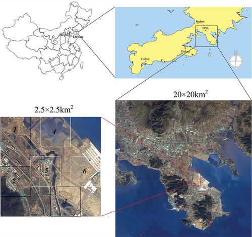
To simulate the supplementary sampling process, the sub-study area (2.5 × 2.5 km²) was first used to conduct a detailed analysis. The sub-study area was divided into six sub-images with a resolution of 300 ×300 pixels. The sub-images were further divided into two groups: Group A comprises sub-images 1, 2, and 3; and Group B comprises sub-images 4, 5, and 6. Group A represents the initial sample set, which contains basic class information; and Group B is the supplementary sample set, which is used to supplement the diversity of spectral signatures. The validation dataset comprises 2695 pixels obtained by random sampling.

3. Methodology

3.1. The structure of AUSD learning system

AUSD learning system models the remote-sensing data using a more expressive Gaussian mixture assumption. The parameters of subclasses are obtained by grid-based density estimation. To learn the supplementary sample sets continuously, a short-term storage (STS) and a long-term storage (LTS) are introduced according to the multi-store strategy and the time duration of material in memory. The topological graph of AUSD is shown in Figure 2.

Figure 2. Topological graph of AUSD (a) Calibration phase and (b) Validation phase.

The STS is a temporary layer used to store current subclasses’ information and will be covered when the next calibration set is inputted. The existing subclasses are stored in the permanent LTS layer, which is used to retain valuable information of the entire model. Subclasses in LTS can be adjusted by supplementary information. Specifically, if a subclass in STS is similar to the one in LTS, then both subclasses will be merged into a corresponding subclass in LTS. Otherwise, a new subclass will be created in LTS. After the measurement of symmetric KL divergence, either the existing subclasses are updated or new subclasses are created. Figure 3 illustrates the implementation process of the proposed AUSD.

Figure 3. Flow diagram of AUSD.

3.2. The mathematical description of AUSD learning system

In the initial transition, the pixels are grouped into homogeneous segments by clustering or classifying the feature vectors in the selected multidimensional feature space.

3.2.1. Gaussian assumption

The distribution of a single LULC class is assumed to be a mixture Gaussian model, and its subclass satisfy the Gaussian distribution (Tuia, Pasolli, and Emery 2011; Vigdor and Lerner 2007). In this part, the derivations of equations referred to the machine learning book by Bishop (2006).

The input feature vector is . is the set of LULC classes. Assume that class consists of Gaussian subclasses ; thus, , where is the positive-definite covariance matrix and is the mean of the subclass . The distribution of a random variable is a mixture of Gaussians, and its density function is written as follows:

(1)

such that the parameter set is , where .

3.2.2. Grid-based unimodal subclass decomposition

A calibration set with samples is , where is the feature vector and is the label. Each dimension of the feature spaces is partitioned into m × m hyper-rectangular cells. Figure 4 illustrates an example of the grid partition in two dimensions of two subclasses. Each cell is described by three components namely, location index , intensity , and state .

Figure 4. Grid partition of subclasses (a) two-dimensional and (b) three-dimensional. For full color versions of the figures in this paper, please see the online version.

The neighbor cell of is defined as follows:

(2)

where , which is the distance between cells. If , then it is the Chebyshev distance.

Thus, all connected cells surrounding the centerd cell are considered. For the convenience of calculation, the entire calibration set is separated into class sets according to labels y. denotes the kth class set with samples and indicates the mean intensity of every class in each cell. With the increase of , is regarded as a non-decreasing positive integer sequence that satisfies the following conditions:, , and . is a particular solution to satisfy these conditions. Let such that the number of intervals for each dimension is defined as: .

The length of an interval for dimensions can be calculated as , where each element of vector is the maximum sample value for the corresponding dimension, and is the minimum vector. The position of sample is mapped into the as follows:

(3)

where , is the round down operator. denotes that is the candidate for peak cell, whereas denotes that will not be considered when searching for the peak cell. is initialized as 1. The process of searching for the peak cell is described as follows:

• Step 1: The state value will be set to 0 if the intensity of the cell is lower than , which is introduced to limit the computational complexity and the effect of noise.

• Step 2: Build the candidate cell set denoted as . includes all the cells whose state is . Sort the cells in descending order according to the intensity .

• Step 3: Select the first cell in to obtain its index .

• Step 4: Obtain the according to Equation (2) and compare the intensity with those neighbor cells. If and are satisfied, it indicates that gets the maximal intensity. As a conclusion, is a peak cell corresponding to a subclass, then proceeds to step 5. If cannot satisfy the above conditions, then set and return directly to step 3.

• Step 5: Build the subclass and set both states of and cells in to 0; consequently, these cells are excluded from . Return to step 3 to search for the next peak cell until is empty.

The searched number of peak cells is defined as . If only one subclass exists in this class dataset, then the distribution of the current class dataset will have a unimodal density. and maximum likelihood parameters are calculated as follows:

(4)

If more than one peak cell are in the grid, then .

(5)

To simplify the calculation process, dummy variable is introduced as follows:

(6)

Then the covariance matrix can be expressed as follows:

(7)

All these subclasses are initiated by peak cell samples. The final distributions need to be adjusted by remainder of samples. Given that sample , the posterior probability corresponding to each subclass is expressed as follows:

(8)

where . The discriminant function (Bishop 2006) is defined as follows:

(9)

where , , and .

is the subclass that obtains the maximal value of Equation (9), which is chosen as the winning subclass.

(10)

Then, the parameters of this subclass are updated as follows:

(11)

All parameters describing the distribution of current subclasses are stored in STS and will be compared with the parameters of subclasses stored in LTS.

3.2.3. Subclass adjustment based on supplementary calibration set

denotes the jth existing subclass in class , and symmetric KL divergence is introduced to determine whether a current subclass must be merged into an existing subclass .

(12)

Under Gaussian distribution, the symmetric divergence that measures the average separability for both and is expressed as follows:

(13)

Current subclass is compared with all to find the minimum .

(14)

If , then the current subclass will be merged into the existing subclass based on the following:

(15)

If , then the current subclass is added as a new subclass into LTS. Set ; .

3.2.4. Validation process of LULC classification

In the validation process, existing subclasses in LTS are used to classify the validation set. The labels are obtained by the maximum posterior probability.

(16)

Then, the posterior probability of class can be calculated as follows:

(17)

where . Then, the label of validation sample is expressed as follows (Zhao et al. 2013):

(18)

4. Results and discussions

4.1. Numerical experiments

A numerical experiment was conducted to validate the continuous learning performance of AUSD using simulated data in a 2D feature space. One class containing several subclasses was used to reflect the complexity of data. Each subclass was simulated by the Gaussian data, as shown in Figure 5. Five groups of data from two classes are listed in Table 1, where Data 3 and 5 belong to the same subclass. Parameters of merged data are listed in the last row of Table 1.

Table 1. The number, mean, covariance matrix, and label of simulated Gaussian data in numerical experiment.

	Number	Mean		Covariance matrix		Label
Data1	500	1.9372	−2.0096	4.9036	3.0525	1
				3.0525	3.8927
Data2	300	1.9770	−6.0832	0.6681	0.2257	1
				0.2257	0.6837
Data3	700	9.0432	−5.4291	5.3442	−2.1361	2
				−2.1361	5.3760
Data4	300	−2.0320	1.0542	3.9649	−0.8505	2
				−0.8505	1.9562
Data5	100	9.0235	−5.7989	5.1925	−2.0193	2
				−2.0193	5.0684
Data3	800	8.9558	−5.4175	5.2341	−2.1225	2
Data5				−2.0317	5.4569

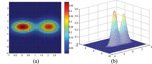
Figure 5. Distribution of Gaussian data (a) original data and (b) data with supplementation. For full color versions of the figures in this paper, please see the online version.

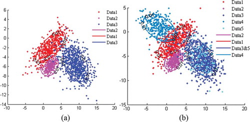
To simulate the continuous learning process, Data 1, 2, and 3 were used as the original data (Figure 5(a)) and Data 4 and 5 were considered as supplementary data (Figure 5(b)). Class 1 comprised two subclasses, and Class 2 had only one subclass. With supplementary data, a new subclass for class 2 and Data 5 may be merged into a subclass created by the original Data 3. Figure 5 illustrates the isoprobability contour plots wherein the probability is at 0.01.

The learning result of original data from AUSD is shown in Table 2. Three subclasses were stored in LTS under the supervision of two kinds of labels. As shown in Figure 6(a), AUSD found three Gaussian components corresponding to three subclasses. AUSD clearly decomposed the mixture density into unimodal subclasses with accurate peak position and distribution form.

Table 2. AUSD learning result (number, mean, covariance matrix, and label) of original data.

	Number	Mean		Covariance matrix		Label
Subclass 1	488	2.0230	−1.7519	5.5012	2.9650	1
(Data 1)				2.9650	3.6453
Subclass 2	312	1.9698	−5.9994	0.9036	0.3039	1
(Data 2)				0.3039	0.5887
Subclass 3	700	9.2055	−5.6940	5.0941	−1.8774	2
(Data 3)				−1.8774	4.8736

Figure 6. Results of data density estimation for the first and second dimensions (a) data distribution histogram and the density estimation curve of original data, (b) data distribution histogram and the density estimation curve of data with supplementation, (c) isoprobability contour plots of original data and data with supplementation. For full color versions of the figures in this paper, please see the online version.

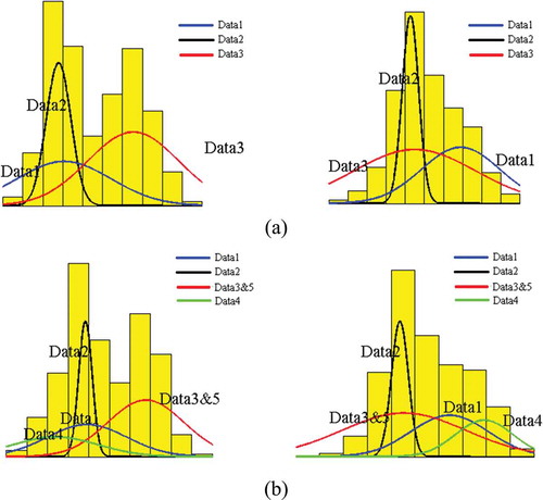
To further simulate the supplementary calibration set, Data 4 and 5 were processed by AUSD. The learning results of the original and supplementary data are listed in Table 3. Given that Data 3 and 5 were drawn from the same distribution, then they could merge into one subclass. One additional subclass was created to represent Data 4. As shown in Figure 6(b), AUSD effectively learned supplementary data by mining the unimodal subclasses.

Table 3. AUSD Learning result (number, mean, covariance matrix, and label) of original data and supplementary data.

	Number	Mean		Covariance matrix		Label
Subclass 1	488	2.0230	−1.7519	5.5012	2.9650	1
(Data 1)				2.9650	3.6453
Subclass 2	312	1.9698	−5.9994	0.9036	0.3039	1
(Data 2)				0.3039	0.5887
Subclass 3	799	9.1696	−5.6157	5.0701	−1.8468	2
(Data 3 and 5)				−1.8468	4.8715
Subclass 4	301	−2.0034	0.9740	4.1120	−0.9534	2
(Data 4)				−0.9534	2.1559

4.2. Remote-sensing image LULC classification experiment

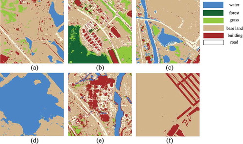
First, the continuous learning ability of AUSD was verified using a sub-study image. Classification results for six sub-images (as shown in Figure 7) were obtained using the corresponding intermediate results of AUSD.

Figure 7. AUSD classification images of Groups A and B: (a) sub-image 1, (b) sub-image 2, (c) sub-image 3, (d) sub-image 4, (e) sub-image 5, (f) sub-image 6. Each sub-image is in the size of 300 × 300 pixels. For full color versions of the figures in this paper, please see the online version.

AUSD has a stronger ability to describe categories and achieves an improved division of classes. Two classification images of AUSD are shown in Figure 8(a). Upon learning Group A, the model obtained the basic recognition of main land cover classes but failed to recognize the classes with spectral changes. For example, water was incorrectly recognized as bare land in many pixels. The model achieved better performance after adjusting by Group B, which reflected the performance of continuous learning on the sample sets.

Figure 8. Preliminary images and final classification images of (a) proposed AUSD, (b) SVM, (c) MLC, (d) NB, (e) ELM, (f) FAM, (g) KNN, (h) DT. Each sub-image is in the size of 1000 × 1000 pixels. For full color versions of the figures in this paper, please see the online version.

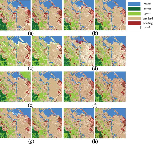
Second, AUSD was compared with several traditional pattern classification methods such as SVM, maximum likelihood classifier (MLC), naive Bayes classifier (NB), extreme learning machine (ELM), fuzzy ARTMAP (FAM) (Seto and Liu 2003), k-nearest neighbors (KNN) algorithm, and decision tree (DT). Parameters of these algorithms were adjusted by 10-fold cross validation. Figure 8(b–h) shows the classification results of these algorithms.

Preliminary results were obtained by models learned from Group A. Influenced by the reclamation project; water containing suspended sediments has special spectral characteristics. Misclassifications were generally caused by the incompleteness of the calibration set in the preliminary results of all methods. Group B was then added to improve the performance of classifiers. Both the preliminary and final results illustrate that AUSD (Figure 8(a)) is more effective than SVM (Figure 8(b)). Obvious misclassifications in Figure 8(c) and (d) occurred because of the limitations of MLC and NB in identifying distributions as unimodal Gaussian distribution.

The classification results of ELM (Figure 8(e)) had good integrity. However, its recognition of water and buildings is worse than the proposed AUSD learning system. FAM is similar to AUSD: The major difference is their sensitivity to statistically overlapping between classes. FAM created 192 nodes, whereas AUSD only created 62 unimodal subclasses, thereby causing the scattered classification images shown in Figure 8(f). Figure 8(g)–(h) shows the results of KNN and DT classifiers. The recognitions of the road by these classifiers are somewhat unclear because the partial model is easily affected by noise and mixed pixels, which is based on local information. Figure 8 shows that the proposed AUSD performs best in considering all kinds of land cover classes.

A confusion matrix was used to obtain Tables 4 and 5. The supplementary samples were important to improve the performance of the classifier. The proposed AUSD method obtained the highest overall accuracy and Kappa coefficient. This accuracy was due to the subclass description ability and reflected the superiority of the proposed model in overcoming difficulties related to spectral complexity.

Table 4. Producer accuracies with Group A calibration set.

	AUSD	SVM	MLC	NB	ELM	FAM	KNN	DT
Water	1.0000	0.9347	0.9946	0.8150	0.7388	0.8599	0.8952	0.8639
Forest	0.9633	0.9306	0.8367	0.8939	0.8041	0.9306	0.9306	0.9143
Grass	0.9143	0.8327	0.9918	0.9878	1.0000	0.9592	0.9347	0.8286
Bare land	0.9197	0.9401	0.8204	0.3946	0.9891	0.8626	0.9020	0.8558
Building	0.9020	0.7857	0.5061	0.5857	0.6673	0.7531	0.8041	0.7102
Road	0.6653	0.5592	0.7673	0.4898	0.5673	0.4367	0.5796	0.4367
OA	0.9187	0.8653	0.8230	0.6519	0.8082	0.8182	0.8586	0.7963
Kappa	0.8972	0.8299	0.7782	0.5729	0.7612	0.7696	0.8222	0.7418

AUSD: Adaptive unimodal subclass decomposition; SVM: support vector machine; MLC: maximum likelihood classifier; NB: naive Bayes; ELM: extreme learning machine; FAM: fuzzy ARTMAP; KNN: k-nearest neighbors; DT: decision tree.

Table 5. Producer accuracies with Group A calibration set and Group B calibration set.

	AUSD	SVM	MLC	NB	ELM	FAM	KNN	DT
Water	1.0000	1.0000	0.9973	0.9973	0.9905	1.0000	1.0000	1.0000
Forest	0.9184	0.9265	0.8245	0.8694	0.8041	0.9224	0.9306	0.9020
Grass	0.9755	0.9020	0.9959	0.9959	1.0000	0.9551	0.9388	0.8041
Bare land	0.9646	0.9810	0.7932	0.5265	0.9918	0.8694	0.9510	0.9551
Building	0.9306	0.9143	0.5041	0.6245	0.6531	0.8735	0.9000	0.8898
Road	0.6041	0.5469	0.7184	0.3755	0.4327	0.4735	0.4653	0.4490
OA	0.9321	0.9224	0.8108	0.7328	0.8627	0.8824	0.9080	0.8909
Kappa	0.9139	0.9016	0.7637	0.6665	0.8247	0.8515	0.8833	0.8609

AUSD: Adaptive unimodal subclass decomposition; SVM: support vector machine; MLC: maximum likelihood classifier; NB: naive Bayes; ELM: extreme learning machine; FAM: fuzzy ARTMAP; KNN: k-nearest neighbors; DT: decision tree.

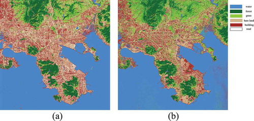
Finally, AUSD and SVM were applied to acquire the classification results of the entire image because they obtained the best results in the sub-study image. Two sets of 4500 data points labeled by random sampling were used to build the calibration and validation sets. The confusion matrices of AUSD and SVM are shown in Tables 6 and 7. The classification results are shown in Figure 9.

Table 6. The confusion matrix of AUSD of the entire image experiment.

		Predictions
		Water	Forest	Grass	Bare land	Building	Road	PA
Actual conditions	Water	997	1	0	0	2	0	0.9970
	Forest	0	1386	100	1	12	1	0.9240
	Grass	0	77	921	0	2	0	0.9210
	Bare land	0	0	19	408	59	14	0.8160
	Building	11	14	10	34	2311	120	0.9244
	Road	0	0	1	8	71	420	0.8400
	UA	0.9891	0.9378	0.8763	0.9047	0.9406	0.7568
OA		0.9204
Kappa		0.8976

Table 7. The confusion matrix of SVM of the entire image experiment.

		Predictions
		Water	Forest	Grass	Bare land	Building	Road	PA
Actual conditions	Water	775	0	0	0	225	0	0.7750
	Forest	0	1156	6	0	338	0	0.7707
	Grass	0	3	780	0	217	0	0.7800
	Bare land	0	0	0	387	112	1	0.7740
	Building	0	0	0	2	2498	0	0.9992
	Road	0	0	0	0	106	394	0.7880
	UA	1.0000	0.9974	0.9924	0.9949	0.7145	0.9975
OA		0.8557
Kappa		0.8067

Figure 9. Classification images for the entire study area: (a) proposed AUSD, (b) SVM. Each image is in the size of 8000 × 8000 pixels. For full color versions of the figures in this paper, please see the online version.

5. Conclusion

AUSD learning system was proposed to overcome modeling limitations caused by the incompleteness of calibration set and the complexity of spectral signatures. Two effects were achieved by AUSD:

1. LULC classes that contain rich spectral variations could be recognized as the combination of different subclasses, and AUSD model could identify subclasses more accurately.

2. The model could be adapted to supplementary samples by adjusting the parameters of existing subclasses or building new subclasses. AUSD model could obtain more plasticity to adapt to extended study areas.

Numerical experiments on mixed Gaussian data showed that AUSD learning system effectively separated subclasses to develop the mixture model and adapted to additional data components. The experiments on high-resolution remote-sensing images validated that AUSD model could obtain accurate results and overcome the problems of spectral complexity more effectively than traditional classification algorithms.

In addition, the continuous learning ability of AUSD allows it to be easily developed into an active learning system. Our future study will focus on optimizing the definition of a calibration set by labeling a minimum number of high-quality samples and extending AUSD learning system to a more automatically active learning method.

Acknowledgments

We are grateful to anonymous reviewers and the editor for their valuable comments, which have greatly improved the quality of this manuscript.

Disclosure statement

No potential conflict of interest was reported by the authors.

Additional information

Funding

This work was supported by the project of the National Natural Science Foundation of China: [Grant number 61374154]; the Special Fund for Basic Research on Scientific Instruments of the National Natural Science Foundation of China: [Grant number 51327004].

References

- Azari, M., A. Tayyebi, M. Helbich, and M. A. Reveshty. 2016. “Integrating Cellular Automata, Artificial Neural Network and Fuzzy Set Theory to Simulate Threatened Orchards: Application to Maragheh, Iran.” GIScience & Remote Sensing 53 (2): 183–205. doi:10.1080/15481603.2015.1137111.
- Bishop, C. M. 2006. Pattern Recognition and Machine Learning. Singapore: Springer.
- Bruzzone, L., and M. Marconcini. 2009. “Toward the Automatic Updating of Land-Cover Maps by a Domain-Adaptation SVM Classifier and a Circular Validation Strategy.” IEEE Transactions on Geoscience and Remote Sensing 47 (4): 1108–1122. doi:10.1109/Tgrs.2008.2007741.
- Chang, N. B., M. Han, W. Yao, L. C. Chen, and S. Xu. 2010. “Change Detection of Land Use and Land Cover in an Urban Region with SPOT-5 Images and Partial Lanczos Extreme Learning Machine.” Journal of Applied Remote Sensing 4 (1): 043551-043551-15. doi:10.1117/1.3518096.
- Cheng, G., L. Guo, T. Zhao, J. Han, H. Li, and J. Fang. 2013. “Automatic Landslide Detection from Remote-sensing Imagery Using a Scene Classification Method Based on BoVW and pLSA.” International Journal of Remote Sensing 34 (1): 45–59. doi:10.1080/01431161.2012.705443.
- Du, Y., D. Wu, F. Liang, and C. Li. 2013. “Integration of Case-based Reasoning and Object-based Image Classification to Classify SPOT Images: A Case Study of Aquaculture Land Use Mapping in Coastal Areas of Guangdong Province, China.” GIScience & Remote Sensing 50 (5): 574–589. doi:10.1080/15481603.2013.842292.
- Giri, C., B. Pengra, J. Long, and T. R. Loveland. 2013. “Next Generation of Global Land Cover Characterization, Mapping, and Monitoring.” International Journal of Applied Earth Observation and Geoinformation 25: 30–37. doi:10.1016/j.jag.2013.03.005.
- Grossberg, S. 2013. “Adaptive Resonance Theory: How a Brain Learns to Consciously Attend, Learn, and Recognize a Changing World.” Neural Networks 37: 1–47. doi:10.1016/j.neunet.2012.09.017.
- Huang, X., Q. Lu, and L. Zhang. 2014. “A Multi-index Learning Approach for Classification of High-resolution Remotely Sensed Images Over Urban Areas.” ISPRS Journal of Photogrammetry and Remote Sensing 90: 36–48. doi:10.1016/j.isprsjprs.2014.01.008.
- Hussain, E., and J. Shan. 2015. “Object-based Urban Land Cover Classification Using Rule Inheritance Over Very High-resolution Multisensor and Multitemporal Data.” GIScience & Remote Sensing 53 (2): 1–19. doi:10.1080/15481603.2015.1122923.
- Inglada, J. 2003. “Change Detection on SAR Images by Using a Parametric Estimation of the Kullback-Leibler Divergence.” IEEE Proceedings of International Geoscience and Remote Sensing Symposium 6: 4104–4106. doi:10.1109/IGARSS.2003.1295376.
- Kullback, S., and R. A. Leibler. 1951. “On Information and Sufficiency.” The Annals of Mathematical Statistics 22 (1): 79–86. doi:10.1214/aoms/1177729694.
- Li, J., J. M. Bioucas-Dias, and A. Plaza. 2013. “Spectral–spatial Classification of Hyperspectral Data Using Loopy Belief Propagation and Active Learning.” IEEE Transactions on Geoscience and Remote Sensing 51 (2): 844–856. doi:10.1109/TGRS.2012.2205263.
- Li, M., J. Im, and C. Beier. 2013. “Machine Learning Approaches for Forest Classification and Change Analysis Using Multi-temporal Landsat TM Images Over Huntington Wildlife Forest.” GIScience & Remote Sensing 50 (4): 361–384. doi:10.1080/15481603.2013.819161.
- Liu, D., M. Kelly, and P. Gong. 2006. “A Spatial–temporal Approach to Monitoring Forest Disease Spread Using Multi-temporal High Spatial Resolution Imagery.” Remote Sensing of Environment 101 (2): 167–180. doi:10.1016/j.rse.2005.12.012.
- Liu, Y., and X. Li. 2014. “Domain Adaptation for Land Use Classification: A Spatio-temporal Knowledge Reusing Method.” ISPRS Journal of Photogrammetry and Remote Sensing 98: 133–144. doi:10.16/j.isprsjprs.2014.09.013.
- Mishra, D. R., S. Narumalani, D. Rundquist, and M. Lawson. 2005. “Characterizing the Vertical Diffuse Attenuation Coefficient for Downwelling Irradiance in Coastal Waters: Implications for Water Penetration by High Resolution Satellite Data.” ISPRS Journal of Photogrammetry and Remote Sensing 60 (1): 48–64. doi:10.1016/j.isprsjprs.2005.09.003.
- Otukei, J. R., and T. Blaschke. 2010. “Land Cover Change Assessment Using Decision Trees, Support Vector Machines and Maximum Likelihood Classification Algorithms.” International Journal of Applied Earth Observation and Geoinformation 12: S27–S31. doi:10.1016/j.jag.2009.11.002.
- Pal, M., A. E. Maxwell, and T. A. Warner. 2013. “Kernel-based Extreme Learning Machine for Remote-sensing Image Classification.” Remote Sensing Letters 4 (9): 853–862. doi:10.1080/2150704X.2013.805279.
- Phillips, R. D., L. T. Watson, D. R. Easterling, and R. H. Wynne. 2014. “An SMP Soft Classification Algorithm for Remote Sensing.” Computers & Geosciences 68: 73–80. doi:10.1016/j.cageo.2014.03.010.
- Salmon, J. M., M. A. Friedl, S. Frolking, D. Wisser, and E. M. Douglas. 2015. “Global Rain-fed, Irrigated, and Paddy Croplands: A New High Resolution Map Derived from Remote Sensing, Crop Inventories and Climate Data.” International Journal of Applied Earth Observation and Geoinformation 38: 321–334. doi:10.1016/j.jag.2015.01.014.
- Seto, K. C., and W. Liu. 2003. “Comparing ARTMAP Neural Network with the Maximum-likelihood Classifier for Detecting Urban Change.” Photogrammetric Engineering & Remote Sensing 69 (9): 981–990. doi:10.14358/PERS.69.9.981.
- Su, Y., X. Chen, C. Wang, H. Zhang, J. Liao, Y. Ye, and C. Wang. 2015. “A New Method for Extracting Built-up Urban Areas Using DMSP-OLS Nighttime Stable Lights: A Case Study in the Pearl River Delta, Southern China.” GIScience & Remote Sensing 52 (2): 218–238. doi:10.1080/15481603.2015.1007778.
- Tuia, D., E. Pasolli, and W. J. Emery. 2011. “Using Active Learning to Adapt Remote Sensing Image Classifiers.” Remote Sensing of Environment 115 (9): 2232–2242. doi:10.1016/j.rse.2011.04.022.
- Vigdor, B., and B. Lerner. 2007. “The Bayesian ARTMAP.” IEEE Transactions on Neural Networks 18 (6): 1628–1644. doi:10.1109/Tnn.2007.900234.
- Wagner, W., A. Ullrich, V. Ducic, T. Melzer, and N. Studnicka. 2006. “Gaussian Decomposition and Calibration of a Novel Small-footprint Full-waveform Digitising Airborne Laser Scanner.” ISPRS Journal of Photogrammetry and Remote Sensing 60 (2): 100–112. doi:10.1016/j.isprsjprs.2005.12.001.
- Xu, J., R. Hang, and Q. Liu. 2014. “Patch-based Active Learning (PTAL) for Spectral-spatial Classification on Hyperspectral Data.” International Journal of Remote Sensing 35 (5): 1846–1875. doi:10.1080/01431161.2013.879349.
- Zhao, K., D. Valle, S. Popescu, X. Zhang, and B. Mallick. 2013. “Hyperspectral Remote Sensing of Plant Biochemistry Using Bayesian Model Averaging with Variable and Band Selection.” Remote Sensing of Environment 132: 102–119. doi:10.1016/j.rse.2012.12.026.